HyperCP: A high-rate spectrometer for the study of charged hyperon and kaon decays
The Fermilab HyperCP Collaboration

Abstract

The HyperCP experiment (Fermilab E871) was designed to search for rare phenomena in the decays of charged strange particles, in particular CP violation in $\Xi$ and $\Lambda$ hyperon decays with a sensitivity of $10^{-4}$. Intense charged secondary beams were produced by 800 GeV/$c$ protons and momentum-selected by a magnetic channel. Decay products were detected in a large-acceptance, high-rate magnetic spectrometer using multiwire proportional chambers, trigger hodoscopes, a hadronic calorimeter, and a muon-detection system. Nearly identical acceptances and efficiencies for hyperons and antihyperons decaying within an evacuated volume were achieved by reversing the polarities of the channel and spectrometer magnets. A high-rate data-acquisition system enabled 231 billion events to be recorded in twelve months of data-taking.
PACS: 07.05.Fb, 29.30.Aj, 29.40.Cs, 29.40.Mc, 29.40.Vj
Keywords: HyperCP; Magnetic spectrometer; Hadronic calorimeter; Hyperon CP violation; Rare hyperon and kaon decays; Fermilab

, , , , , , , , , , , , , , , , , , , , , , , , , , , , , , , , , , , , ,

1 Introduction

Although expected to be ubiquitous in weak decays, CP violation is a small effect, and thus far it has been observed only in the decays of neutral $K$ and $B$ mesons. Searches for (and perhaps discoveries of) this phenomenon in the decays of other particles will provide new insights and will help to determine whether the phase in the Cabibbo–Kobayashi–Maskawa quark mixing matrix [1] is the sole source of CP violation, or whether there are other sources. Many beyond-the-standard-model theories predict CP-violating effects, often with larger signals than found in standard-model calculations. Hyperon decays offer promising possibilities for CP-violation searches: hyperons are copiously produced and readily detected, and their decays are particularly sensitive to certain exotic sources of CP violation [2].

The primary goal of the HyperCP experiment (Fermilab E871) was to search for CP violation in $\Xi$ and $\Lambda$ hyperon decays with a sensitivity far beyond previous limits, and at which some theories predict an effect. The search method was to compare the asymmetries in proton and antiproton decay distributions in $\Lambda$ $\rightarrow$ $p$$\pi^{-}$ and $\overline{\Lambda}$ $\rightarrow$ $\overline{p}$$\pi^{+}$ decays, where the $\Lambda$ and $\overline{\Lambda}$ were produced from unpolarized $\Xi^{-}$ and $\overline{\Xi}$⁺ decays. The signature for CP violation is a nonzero value of $\makebox{${A}_{\Xi\Lambda}$}=\makebox{$(\makebox{$\alpha_{\Xi}$}\makebox{$\alpha_{\Lambda}$}-\makebox{$\overline{\alpha}_{\Xi}$}\makebox{$\overline{\alpha}_{\Lambda}$})/(\makebox{$\alpha_{\Xi}$}\makebox{$\alpha_{\Lambda}$}+\makebox{$\overline{\alpha}_{\Xi}$}\makebox{$\overline{\alpha}_{\Lambda}$})$}$, where $\alpha_{\Xi}$$\alpha_{\Lambda}$ and $\overline{\alpha}_{\Xi}$$\overline{\alpha}_{\Lambda}$ are, respectively, the magnitudes of the asymmetries in the proton and antiproton angular distributions in the $\Lambda$ and $\overline{\Lambda}$ rest frames. To achieve the desired statistical sensitivity of $10^{-4}$ in ${A}_{\Xi\Lambda}$, the HyperCP spectrometer was designed to operate at very high rates. To keep biases below the statistical sensitivity an apparatus with minimal differences in acceptances and efficiencies for $\Xi^{-}$ and $\overline{\Xi}$⁺ decays was also essential. HyperCP recorded 2.5 billion $\Xi^{-}$ and $\overline{\Xi}$⁺ decays; the two best previous searches for CP violation in hyperon decays had datasets of 280 000 $\Xi^{-}$ and $\overline{\Xi}$⁺ events (E756 [3]) and 96 000 $\Lambda$ and $\overline{\Lambda}$ events (PS185 [4]).

An experiment optimized for the physics just described inevitably records large numbers of charged kaon and $\Omega$ decays as well. Hence the spectrometer was designed to have good acceptance for such decays. Also, a simple muon-detection system was added to the spectrometer to allow searches for rare and forbidden kaon and hyperon decays with muonic final states at the level of $\mathcal{O}(10^{-7})$.

HyperCP was approved in June 1994. A new spectrometer was fabricated in two-years’ time, with beam first delivered to the experiment in November 1996. Following a five-month running-in period, data were taken from April to August 1997 and, after minor upgrades, from June 1999 to January 2000. We describe here the 1999 spectrometer and, where appropriate, point out the differences between the apparatus used in the two runs. Further details of the HyperCP data acquisition system can be found in [31, 32, 33]; forthcoming papers will provide thorough descriptions of the HyperCP calorimeter and wire chambers.

2 Overview of the Spectrometer

The experiment was mounted at Fermilab in the Meson Center beamline. The overall layout of the HyperCP apparatus is shown in Fig. 1; Table 1 gives the $z$ positions of the spectrometer elements. The target area was in enclosure MC6 of the Meson Detector Building and was surrounded by thick shielding. The HyperCP spectrometer was in enclosure MC7, which extended beyond the building. Because this enclosure was rather narrow and could not be enlarged, it constrained certain aspects of the spectrometer design. Cables from the spectrometer passed over a bridge to the Electronics Hall in enclosure MP7, where the data were digitized by the front-end elements of the data-acquisition (DAQ) system. Fiber-optic cables carried the digitized data from the Electronics Hall to the Control Room, which was three connected Porta-Kamp trailers [5] alongside enclosure MC8. Radiation levels precluded beam-on occupancy of the Detector Hall, but the Electronics Hall could be occupied even when beam was being delivered to the experiment; this was an important consideration for efficient trigger and DAQ-system commissioning and maintenance.

Elevation and plan views of the HyperCP spectrometer are shown in Fig. 2. Intense charged secondary beams with mean momenta of about 160 GeV/$c$ were produced by 800 GeV/$c$ protons striking $2{\times}2$ mm² targets, with the secondaries charge- and momentum-selected by means of a curved channel embedded in a dipole magnet (Hyperon Magnet). The central orbit of the secondary beam emerged from the channel at a 19.51 mrad angle above the horizontal. The mean momentum of the secondary beam was chosen to be fairly low, corresponding to a small value of $x_{F}$ (${\approx}0.2$), in order to minimize the differences between the $\Xi^{-}$ and $\overline{\Xi}$⁺ yields, but to be still high enough that the acceptance was relatively good. Typically the incident proton beam was collinear with the entrance axis of the channel, but about 10% of the data were taken at nonzero targeting angles in order to produce polarized hyperons. The secondary-beam intensity was usually ${\approx}$13 MHz, dominantly pions in the negative-polarity beam and with roughly equal numbers of pions and protons in the positive-polarity beam. It was dumped in a massive concrete and iron structure between enclosures MC7 and MC8. To switch between the positive and negative secondary-beam polarities, the polarities of both the Hyperon and Analyzing Magnets were reversed, and target lengths were changed in order to keep the intensity of the secondary beam the same. This resulted in nearly identical acceptances and efficiencies for hyperons and antihyperons, which was essential for minimizing biases.

A high-rate magnetic spectrometer of nine multiwire proportional chambers (MWPCs) and two dipole magnets (Analyzing Magnets) situated back-to-back followed a 13 m long evacuated pipe (Vacuum Decay Region). A simple trigger, used to select candidate $\Xi$ $\rightarrow$ $\Lambda$$\pi$ $\rightarrow$ $p$$\pi$$\pi$ decays as well as other charged hyperon and kaon decays, required the coincidence of at least one charged particle each on the left and right sides of the secondary beam. Left and right are defined with respect to an observer looking downstream along the beam line, and are also referred to respectively as the “same-sign” and “opposite-sign” sides, or pion and proton sides, since both pions from the $\Xi$ decay had the same charge as the secondary beam, while the proton had the opposite charge and hence was deflected in the opposite direction by the field of the Analyzing Magnets. The trigger employed two hodoscopes (Same-Sign and Opposite-Sign Hodoscopes), situated on either side of the secondary beam, and located sufficiently far downstream of the Analyzing Magnets that the proton and pions from the $\Xi$ decays had all separated from the secondary beam. To suppress backgrounds from interactions of the secondary beam with material in the spectrometer, the trigger also required a minimum energy deposit in a hadronic calorimeter (Hadronic Calorimeter). Care was taken to keep the material in the spectrometer at a minimum, with helium-filled bags placed between the wire chambers and the hodoscopes, and in the apertures of the Analyzing Magnets. The total material in the spectrometer, including helium bags, from the collimator exit to the Opposite-Sign Hodoscope, was about 2.3% of an interaction length and 4.7% of a radiation length.

A muon-detection system consisted of two stations on either side of the charged secondary beam. Each station had three layers of proportional-tube planes interspersed with iron shielding. Muon triggers were formed with signals from two planes of scintillation hodoscopes located behind the iron absorbers in each station. Just to the rear of the Muon Stations were two hodoscopes (collectively called the Beam Hodoscope) that were centered on the secondary beam and used to measure its intensity.

A fast front-end latch system coupled with a small event size and a high-rate data-acquisition system enabled up to 100 000 events per spill second to be recorded on magnetic tape. A total of 231 billion events were written during the 1997 and 1999 runs.

3 Beam and Beamline

After acceleration to 800 GeV/$c$ in the Fermilab Tevatron, primary protons were extracted at a rate of about $2.5{\times}10^{11}$ s^-1 and sent to the Switchyard. A small fraction, typically fewer than $1{\times}10^{10}$ protons/s, were split from the main proton beam and sent to the Meson Center (MC) beamline, whose elements are shown in Fig. 3. Upon leaving the Switchyard, the Meson Center beam rose gradually and was deflected back into the horizontal by magnets in enclosure M01. The beam was transported to enclosure MC6 (Fig. 1), where the secondary beam was created.

The primary proton beam was bunched by the 53 MHz RF cavities of the Tevatron into “RF buckets,” each about 1 ns wide and separated by 18.9 ns. Typically about $1{\times}10^{11}$ 800 GeV/$c$ protons were delivered in a 40-second spill, producing a secondary beam of ${\approx}$13 MHz intensity (at a $0^{\circ}$ targeting angle). Between spills was a 40-second interspill period during which no beam was delivered to the experiment.

The primary-beam intensity was monitored by both an ion chamber (IC) and a secondary-emission monitor (SEM) located in the MC6 enclosure. These devices integrated charge during the spill and were calibrated to give an absolute measure of the total number of protons traversing them per spill. Readings from each were recorded at the end of each spill. The IC began to saturate at instantaneous beam intensities above about $1{\times}10^{10}$ protons/s, and was fully saturated at about $1.3{\times}10^{10}$ protons/s. It was thus not accurate above the nominal operating intensity, but worked well during low-intensity studies. The SEM was used as the primary beam-intensity monitor. It was calibrated (with an uncertainty of $\pm$5%) by sending a known number of protons from the Switchyard to the Meson Center beamline, with all splits to other beamlines disabled.

The secondary beam was created in enclosure MC6 by steering the primary protons onto a target centered on the entrance of a curved channel, or collimator. The collimator was installed within a dipole magnet, MC6SW. (See Fig. 4 for an elevation view of the secondary-beam forming area.) To create an unpolarized hyperon beam (the usual mode of operation), protons were incident on the target at $0^{\circ}$ relative to the entrance axis of the collimator. For about 10% of the running time (“polarized” running), nonzero horizontal targeting angles of ${\pm}$3.0 mrad (and to a lesser extent ${\pm}$2.5, ${\pm}$2.0, and ${\pm}$1.0 mrad) were used. The targeting angles were tuned by means of two “angle-varying bend” (AVB) dipole-magnet pairs, horizontal (MC6EW1–2) and vertical (MC6UD1–2), located upstream of MC6SW. The largest possible horizontal (vertical) targeting angle was 3.3 mrad (1.5 mrad). The actual zero-degree horizontal targeting angles were $-0.52$ mrad in the 1997 run and $+0.09$ mrad in the 1999 run. The actual zero-degree vertical targeting angles were very close to zero. The rather large targeting angle in the 1997 run was due to imperfect positioning of the target relative to the entrance axis of the collimator. The maximum angular deviation from the nominal targeting angles, limited by beamline apertures, was 0.48 mrad (0.26 mrad) in the horizontal (vertical) direction. The average angular divergence of the beam was considerably less.

The position and shape of the primary beam were measured using eight segmented-wire ion chambers (SWICs) positioned at various points along the beamline. Each SWIC had one plane of vertical and one of horizontal wires, each with 48 wires spaced 1.0 mm apart, except for the two SWICs closest to the target (MC6WC1 and MC6WC2), which had a 0.5 mm wire pitch. The integrated charge accumulated on each wire was digitized and read out every 4 s during the beam spill and displayed graphically on video monitors at the end of each spill to facilitate beam monitoring and tuning. The charge profiles from five SWICs (MC00WC, MC2WC, MC5WC, MC6WC1, and MC6WC2) were also recorded spill-by-spill by the SlowDA (described in Sec. 13.2). The center of each SWIC with respect to the nominal beam centerline was determined by survey. The position of the target with respect to the SWICs was determined empirically by moving the target (between spills) in steps, either up-down or left-right, and finding the target position at which the interaction rate was maximized. The charge profiles from MC6WC1 and MC6WC2 (also called the target SWICs) were fitted offline spill-by-spill to find the $x$ and $y$ coordinates of the beam centroid at the target $z$ center as well as the targeting angles of the beam with respect to the $z$ axis. The $z$ distance between the target SWICs was 2.5 m, with MC6WC2 located 0.22 m upstream of the center of the target.

Due to sharing of charge across adjacent wires, the SWICs did not accurately measure the true size of the beam. The beam size and shape were determined from target scans (as just described), in which beamline settings were held fixed while the target was moved in horizontal or vertical steps. The fraction of the beam hitting the target was reflected in the counting rates per incident proton of various counters in the spectrometer. One such ratio is plotted versus target location in Fig. 5. Since the target size was well known, these distributions allowed the beam size and shape to be determined. Using this method it was found that the beam at the target was approximately Gaussian in shape, typically with $\sigma_{x}=0.45{\pm}0.08$ mm and $\sigma_{y}=0.38{\pm}0.08$ mm. For comparison, the shape of the beam as measured by the most downstream SWIC (MC6WC2) was Gaussian with $\sigma_{x}=\sigma_{y}=1.8$ mm.

4 Target Assembly

To produce positive and negative secondary beams of comparable intensities, two targets of different lengths were used. To minimize acceptance differences and to reduce attenuation of the produced particles, the targets were kept short. Copper targets of 20 mm and 60 mm lengths were used to produce respectively the positively and negatively charged secondary beams. The transverse dimensions of both targets were 2 mm${\times}$2 mm. The positive- and negative-secondary-beam rates per proton on target differed by less than 5% (see Fig. 6).

The targets were supported by an assembly (Fig. 7) constructed from two sets of 1-mm-thick Kyocera alumina-ceramic plates, each containing laser-drilled [6] circular or semicircular holes, within which the targets were clamped. The two targets, located 24 mm apart horizontally, were each secured at two locations along their length between a central ceramic plate and a ceramic edge strip. Additional holes served as “empty” targets used for background studies and (at an early stage of the experiment) to hold additional targets used in run-condition optimization studies and cross-section measurements. The ceramic plates were bolted onto horizontal 8-mm-thick aluminum bars at the top and the bottom of the target holder.

The target holder was mounted on a precision manipulator that was remotely controlled to move in the vertical and horizontal directions in very fine steps. To prevent the wrong target from being used for a given beam polarity, signals from position sensors in the target system were input to the primary beam safety-interlock system. Once the proper target was in place, it could be moved from its nominal position in the horizontal direction within a range of only $\pm$3.5 mm without disabling the beam. The targets could be repositioned reproducibly to within a few $\mu$m. During normal operation, the temperature of the target was kept below 900 K using a blower delivering 7 m³/min of forced air.

5 Collimator and Hyperon Magnet

A 6.096 m long curved collimator installed within the Hyperon Magnet channeled a charged secondary beam of modest momentum spread from the target to the spectrometer (Fig. 8). The upstream face of the collimator was 0.292 m downstream of the target centers; the targets nominally were centered horizontally and vertically on the entrance aperture of the collimator. The collimator, Hyperon Magnet, and surrounding shielding also served as the dump for those primary-beam protons that did not interact in the target. Due to the width of the Detector Hall and height of the primary beam above the floor, the charged secondary beam had to be deflected upwards. The entire dipole-magnet/collimator assembly was encased in massive iron and concrete shielding to reduce radiation in the surrounding area.

A particle with a trajectory along the center of the collimator channel (central-orbit trajectory) exited at an angle of 19.51 mrad above the horizontal. The center of the downstream aperture of the collimator exit defines the origin of the Spectrometer Coordinate System, which is the coordinate system used to describe the spectrometer elements. The $z$ axis of the Spectrometer Coordinate System coincides with the central-orbit direction at the collimator exit, and hence is at an angle of 19.51 mrad to the horizontal (see Fig. 9). To describe the collimator itself, the Beam Coordinate System is used. It is position dependent, with its $z$ axis tangent to the central-orbit trajectory within the collimator, and hence horizontal at the collimator entrance and inclined at 19.51 mrad at its exit.

Although most of the data were taken with the primary proton beam incident at an angle of zero degrees with respect to the entrance axis of the collimator, a significant amount of data at nonzero targeting angles was also recorded in order to produce polarized $\Xi$ hyperons. These data were taken with the incident proton beam deflected in the horizontal direction and hence lying in the $x$–$z$ plane in the Beam Coordinate System, as shown in Fig. 9. A positive (negative) targeting angle is defined to have $\hat{p}_{pb}{\times}\hat{p}_{sb}$ in the $+\hat{y}$ ($-\hat{y}$) direction, where $\hat{p}_{pb}$ is the primary-proton-beam direction and $\hat{p}_{sb}$ is the secondary-beam direction at the entrance of the collimator. Figure 9 shows the direction of the $\Xi^{-}$ polarization for the two targeting angles as well as the direction of precession. The polarization precessed around the magnetic field direction, and at the exit of the collimator in the Spectrometer Coordinate System, the precessed polarization of $\Xi^{-}$’s produced with a positive (negative) targeting angle was at an angle of about $10^{\circ}$ from the negative (positive) $y$ axis, in the $-z$ ($+z$) direction.

As shown in Fig. 8, the collimator was made up of five segments joined together with steel dowel pins. Each segment consisted of a block of brass or tungsten with an attached cover plate. For ease of fabrication, within each block the arc of the channel was approximated by a series of straight-walled milled slots, each such slot 304.8 mm in length. The dimensions of the slots of each segment are given in Table 2. The outer transverse dimensions of the segments were 46.0 mm (width) by 95.2 mm (height), with the corners along the beam direction rounded to fit into the beam pipe inside the Hyperon Magnet. Segment B (Defining Collimator) and Segment E (Exit Collimator) were made of tungsten. The Defining Collimator served as the primary beam dump. At the design magnetic field, the 800 GeV/$c$ proton beam was dumped 3.6 mm (6.4 mm) below the bottom edge of the rectangular aperture at the upstream end of the Defining Collimator when a positive (negative) secondary beam was selected. The Exit Collimator provided a second iris to clean up the secondary beam. Segment A and the tungsten segments (B and E) were water-cooled. With respect to the center of the entrance aperture of Segment A, the solid angle subtended by the limiting (downstream) aperture of the Defining Collimator was approximately 5.38 $\mu$sr.

To center the target on the entrance aperture of the collimator, the target was stepped through a series of $x$ and $y$ positions, with the proton beam centered on the target at each position. The $\Xi$ momentum and position distributions in the spectrometer for each target position were compared with those generated by Monte Carlo simulations. It was not possible to directly check the resulting position of the target relative to the collimator entrance, as the target area was inaccessible. The target center should have been $x=0.0$ mm and $y=65.16$ mm in the Spectrometer Coordinate System. The actual target positions, determined by tracing reconstructed $\Xi$ trajectories back through the collimator, are given in Table 3. Alignment errors in 1997 caused the target to be mispositioned by $+4.6$ mm in $x$ and $-2.3$ mm in $y$. In 1999 the target positioning was much improved, with the target center at the nominal position within a fraction of a millimeter in both $x$ and $y$.

The Hyperon Magnet within which the collimator was placed was an 11 455 kg B2 dipole magnet [7] fabricated at Fermilab for the Main Ring of the accelerator. Its exterior dimensions were 0.362 m (height) by 0.641 m (width) by 6.071 m (endplate to endplate). It was installed on its side to produce a field in the horizontal (${\pm}\hat{x}$) direction.The charge of the secondary beam was changed by reversing the Hyperon Magnet field direction: when producing a secondary beam of positive (negative) polarity, the magnetic field was in the $+\hat{x}$ ($-\hat{x}$) direction. A current of 4193 A produced a field of 1.667 T. At this field the central-orbit momentum was 156.2 GeV/$c$. After the collimator was installed in the beam pipe of the Hyperon Magnet, the beam pipe was sealed at each end with a 76.2-$\mu$m-thick Kapton window. To minimize scattering of the secondary-beam particles, the beam pipe was filled with flowing helium gas at atmospheric pressure.

The acceptance of the collimator, defined as the fraction of charged particles from the target that cleared the Defining Collimator and emerged from the exit of the channel, is shown as a function of momentum in Fig. 10. Momentum spectra of the reconstructed $\Xi^{-}$ and $\overline{\Xi}{}^{+}$ hyperons from the 1999 run are shown in Fig. 11; the mismatch is due to the different mechanisms for producing a $\Xi^{-}$ and a $\overline{\Xi}{}^{+}$ in proton-nucleon collisions.

The magnetic field of the Hyperon Magnet was monitored by two miniature LPT-141-20-S Hall probes [8]. These were located 0.89 m upstream of the exit of the collimator and centered in $y$ within the milled slot in Segment E shown in Fig. 8. The Hall probes were read out by the SlowDA (described in Sec. 13.2) via serial CAMAC using a DTM-141 teslameter [8]. Figure 12 shows the spill-by-spill average Hall probe readings, as well as the magnet currents, for all of the 1999 positive- and negative-polarity beam spills. The magnitudes of the currents were almost identical between the two polarities: for both the 1997 and 1999 runs, the fractional difference (averaged over all spills) between the positive- and negative-secondary-beam magnet currents was just $0.48{\times}10^{-4}$. The currents were quite stable: the rms deviation was 2.6 A (2.8 A) for the 1999 (1997) run. Unfortunately, the two Hall probes did not exhibit consistent readings: Probe 2 had a 15 G (91 G) higher reading than Probe 1 in the 1999 run for positive (negative) secondary-beam polarity, and a 20.2 G (59.2 G) higher reading in the 1997 run. This is because both probes had a zero-field offset, and Probe 1 was also most likely somewhat misaligned relative to the field direction. Because the Hyperon Magnet was buried under considerable shielding, after the initial installation it was impossible to access the Hall probes to recalibrate and realign them.

Since both probes measured the same field — B2 magnets have a very uniform field — correlations in the two probe readings were used to measure the intrinsic ability of the Hall probes to follow changes in the Hyperon Magnet field. The rms resolution of the probes for tracking such changes was thus found to be 0.8 G in 1997 and 2.0 G in 1999.

6 Vacuum Decay Region

The parent- and daughter-particle decays of interest were required by the analysis software to occur in a fiducial volume within an evacuated decay pipe (Vacuum Decay Region). The 13.005 m long pipe was made up of three straight sections joined together with flanges and a bellows. The upstream, aluminum pipe was 2.195 m long and had an inner diameter of 0.254 m and a wall thickness of 19.05 mm. Its upstream window was titanium, 0.102 m in diameter and 76.2 $\mu$m thick, and located 0.318 m downstream of the collimator exit (about 45 mm downstream of the Hyperon Magnet beam-pipe exit window). The middle segment was a 7.849 m long aluminum pipe of inner diameter 0.305 m and wall thickness 19.05 mm. The last segment, 2.657 m in length, was coupled to the middle segment by a 0.305 m long, 0.305 m diameter bellows. This steel pipe had an inner diameter of 0.584 m and wall thickness of 25.4 mm. The downstream window of the Vacuum Decay Region was made of 0.508 mm thick Kevlar [10] supporting a 0.127 mm thick Mylar sheet coated with 0.100 mm of Al.

The decay pipe was inclined at an angle of 19.51 mrad to the horizontal, so as to lie along the central-orbit line. It was evacuated to below 1 mTorr pressure. Monte Carlo simulations indicated that the hyperon decays of interest were contained laterally within the inner diameter of the pipe with essentially 100% probability.

7 Analyzing Magnets

The momentum of each charged particle passing through the spectrometer was determined using sets of multiwire proportional chambers situated upstream and downstream of a pair of dipole magnets (Analyzing Magnets). Each Analyzing Magnet, of the Argonne National Laboratory BM109 type [11], weighed about 46 000 kg. The exterior dimensions of the steel magnet cores were 2.387 m (width) by 1.321 m (height) by 1.829 m (length). Figure 13 shows a front view of the upstream magnet. The apertures of the Analyzing Magnets were 0.610 m wide by 0.259 m (0.305 m) high in the upstream (downstream) magnet. (For convenience, the upstream and downstream magnets are also referred to as Magnet 1 and Magnet 2, respectively.) The magnets were tilted upward at the 19.51 mrad central-orbit angle. The two magnets were separated in the beam direction by approximately 0.071 m between the face plates and 0.67 m between the steel cores. The upstream (downstream) Analyzing Magnet was run at a current of about 2450 A (2469 A), producing a magnetic field of 1.345 T (1.136 T).

Before the multiwire proportional chambers (described next) were installed, the Analyzing Magnet field profiles were determined on a three-dimensional grid using the Fermilab “Ziptrack” system [12]. The three components of the magnetic field were measured in ${\approx}$25 mm steps in $x$ and $z$ and ${\approx}$100 mm steps in $y$ using three orthogonal Hall probes mounted on a computer-controlled cart that ran through the magnet apertures on an aluminum I-beam. The magnetic field was sampled at 20 382 lattice points. The major component of the magnetic fields at $x=10$ mm, $y=14$ mm is plotted versus $z$ in Fig. 14.

The magnetic field of each Analyzing Magnet was measured during the run using the same-model Hall probes (LPT-141-20-S) as for the Hyperon Magnet; unlike those in the Hyperon Magnet, these probes worked well. The Hall probes were placed in a region of relatively uniform field near the entrance apertures. During each beam spill, they were read out five times, and (except for a few-minute period following each reversal of field polarity) the magnetic fields were found to be quite stable. To maintain equal acceptances for hyperon and antihyperon decays, when the charge of the secondary beam was reversed by reversing the direction of the Hyperon Magnet field, the direction of the Analyzing Magnet fields was also reversed. When running with positive (negative) secondary-beam polarity, the magnetic fields were oriented in the $-\hat{y}$ ($+\hat{y}$) direction.

It was important that the magnitudes of the magnetic fields be the same for positive- and negative-secondary-beam running, in order to minimize potential biases in the CP-violation analyses. Differences between the magnitudes of the Hall-probe readings for the two secondary-beam polarities were indeed small, as shown in Fig. 15 and Fig. 16. The difference between the positive- and negative-secondary-beam polarity Hall-probe values for all 1999 runs, averaged on a spill-by-spill basis, was $-3.3$ G ($-0.9$ G) for Magnet 1 (Magnet 2); in 1997 the same difference was $-2.6$ G ($+2.6$ G). Spill-to-spill variations of the Hall-probe readings were also small: the rms deviation of all spills was 4.3 G (4.7 G) for Magnet 1 (Magnet 2) in 1999, and about a factor of two greater in 1997.

8 Multiwire Proportional Chambers

Charged particles emerging from the Vacuum Decay Region were tracked by nine high-rate, narrow-pitch multiwire proportional chambers (MWPCs). Four MWPCs (C1–C4) were deployed upstream of the Analyzing Magnets, five (C5–C9) downstream. Narrow-pitch MWPCs were used to keep the individual wire rates in the secondary-beam region less than 1 MHz; the pitch was increased by roughly 25% after every second MWPC in order to keep the maximum wire rate approximately the same in each chamber.

To accommodate the increasing spread of the hyperon and kaon decay products, the nine chambers were of four successively larger sizes, with the additional constraint that the MWPCs fit within the dimensions of the preexisting experimental enclosure. Since two (and in one case, three) chambers were built from each design, and each chamber was installed at a different $z$ position, some chambers were oversized; consequently, not all wires were instrumented. Of 24 096 total wires, 19 680 were instrumented.

8.1 Physical Description

The MWPC mechanical data are given in Table 4. Figure 17 shows a front view of C1, which was identical to C2, and similar to the identical pair, C3 and C4, except smaller. Figure 18 shows a front view of C5, which was identical to C6, and similar to the identical triplet, C7–C8, except smaller. The upstream chambers were all mounted on stands fabricated from Unistrut [13] by means of aluminum extensions attached to the chamber front and back plates. The chamber heights and orientation were fine-tuned by means of nuts on threaded rods that connected the stand to the aluminum extensions. Stands for the rear chambers had winches that allowed those heavy chambers to be hoisted up (Fig. 19). The chambers were hung from threaded rods.

All the chambers were constructed similarly. Each MWPC had four anode-wire planes sandwiched by foil cathode planes (see Fig. 20). The four anode planes had wires oriented in three stereoscopic views. The outer two anode planes (X and X^′) had vertical wires, which measured coordinates in the $x$ direction. To enhance momentum resolution, the X wires were offset from those in X^′ by one-half of the wire spacing. The two inner anode planes (U and V) had wires inclined at $\pm 26.57^{\circ}$ ($=\tan^{-1}(1/2)$) with respect to vertical. All wires were gold-plated W-Rh. Two outer, grounded, foil planes terminated the field region and provided for balancing of electrostatic forces. Except in the case of C9, the foils were 25 $\mu$m thick Kapton with a 120 nm thick vapor-deposited Au layer on both sides. The stack of planes was clamped between 12.7 mm thick aluminum jig plates. In the larger chambers, C5–C9, the back jig plate was reinforced by a box beam. The chamber gas volume was sealed by windows composed of a laminate of 25 $\mu$m Mylar and 25 $\mu$m Al with a 12 $\mu$m layer of adhesive. The total material in each chamber was about 0.07% of an interaction length and 0.2% of a radiation length.

The anode and cathode frames were made of fiber-epoxy laminates, 3 mm thick: Stesalit 4411W [14] for the front chambers and FR4 for the rear chambers. The 4411W was produced with a 25 ${\mu}$m (${\approx}$1%) tolerance on the nominal thickness. The FR4 was ordered oversized and then ground down to the desired 3 mm thickness with the same 25 ${\mu}$m tolerance. Copper-clad FR4 was used for the anode frames in the rear chambers. In the upstream chambers the total wire tension did not produce any appreciable distortion of the anode frames. That was not the case for the downstream chambers, which had many more wires, each with a greater tension. Hence, to eliminate relaxation of the anode wire tension due to distortion of the anode frame, in the downstream chambers the anode (and cathode) frames were mounted on dowel pins that were rigidly fixed to the back jig plate.

The anode wires were glued onto the anode frames using Shell Epon 815 Resin and V-40 hardener [15]. In the upstream chambers, pockets were milled out of the anode frames into which circuit boards were glued. The anode wires were soldered to traces on the circuit boards that carried the signals to preamplifiers that were plugged into connectors soldered to the circuit boards. The X and U planes had preamplifiers facing the same direction, whereas the X^′ and V planes had preamplifiers facing the opposite direction. The copper-clad anode frames of the downstream chambers had traces that were etched out and onto which the wires and preamplifier connectors were soldered. Unlike the upstream chambers, all of the preamplifiers faced forward, which was facilitated by having the X^′ and U anode planes extend beyond the X and V anode planes. Card cages attached to the front and back chamber plates held circuit boards that distributed power to the preamplifiers.

Upstream of the Analyzing Magnets, the hyperon and kaon decay products occupied the same region in the MWPCs as the secondary beam, while in the downstream MWPCs the decay products progressively separated from the beam. To reduce the sensitivity to out-of-bucket beam tracks, and to mitigate aging effects [16], C1–C4 were therefore filled with a “fast” gas mixture of CF₄/isobutane in a 50/50 ratio (see Fig. 21). Since a somewhat poorer time resolution could be tolerated in C5–C8, in the 1997 run those chambers were filled with a 50/50 mixture of argon/ethane bubbled through isopropyl alcohol at $-0.7^{\circ}{\rm C}$. In the 1999 run, the downstream chambers also were operated with the fast-gas mixture, with the exception of C7 which remained filled with argon/ethane since it could not tolerate the higher voltage needed for operation with the fast-gas mixture. Gas flow rates corresponded to approximately three volume changes per day. The chamber cathode-plane voltages were provided by Fermilab ES-7109 (“Droege") power supplies. Typical operating voltages are given in Table 4.

Due to concern about possible aging effects, the signal pulse heights of selected wires in the beam region of a few MWPCs were monitored periodically throughout the 1997 and 1999 runs with a ⁵⁵Fe X-ray source. No significant changes were observed.

8.2 MWPC Electronics

Due to the short time available after approval of the experiment in which to assemble the apparatus, the availability of a large, high-speed latch system from a previous experiment, and the desire to separate the preamplifier from the discriminator for noise reasons, the MWPC signal-processing and readout chain was implemented as three distinct units, rather than a fully integrated on-chamber system.

The high rates demanded a fast, high-gain, low-noise preamplifier for the wire chambers. Since only ${\approx}10\%$ of the total avalanche charge is collected in 10 ns, the typical shaping time of an amplifier appropriate for such high-rate conditions, the expected signal was only ${\approx}5\times 10^{4}e$, assuming an avalanche gain of $10^{5}$ and an initial ionization of $5\,e$ (${\approx}2$ clusters). The threshold of the amplifier/discriminator combination was specified to be less than one-fifth of this average signal charge, or $10,000\,e$, and the equivalent noise charge (ENC) of the amplifier had to be sufficiently low that the random (thermal) noise rate at this threshold would not cause excessive hit multiplicity. After a lengthy evaluation period a commercially available preamplifier ASIC (LeCroy MQS104A [17] with four preamplifiers per chip) was chosen because of its ability to meet specifications, low cost, and small footprint. Characteristics of the preamplifier are given in Table 5. Since the LeCroy MQS104A chip was designed to be used in an on-chamber system, a cable driver for the preamplifier card was designed (Fig. 22). The preamplifier card was a compact four-layer surface-mount board of 16 channels. A total of 21 600 preamplifier channels were mounted on 1350 circuit boards. Before the boards were loaded each channel of the LeCroy MQS104A chips were tested for gain, noise, and time response. Approximately 5% of the chips failed and were replaced by LeCroy. Each channel of the assembled boards was tested again, and boards with failed channels were repaired. The results of these tests are shown in Fig. 23.

The preamplifiers were mounted on the chambers at the ends of the anode fanout-circuit-board traces. The amplified analog signals were conveyed through ${\approx}$10 m of twisted-pair flat cable to discriminator/delay cards located in racks in the experiment enclosure. Characteristics of the discriminator cards are given in Table 6. About 100 ns of lumped-constant delay was incorporated on the cards to allow for trigger latency. The binary output signals from the discriminators were conveyed on ${\approx}$60 m of flat cable to a high-speed latch system situated in the Electronics Hall and described in Sec. 13.1.

In such a large system of several thousand high-gain amplifiers, attached to sense-wire “antennae” and packed together in close proximity, the possibility of coherent oscillation is always a concern. Initially the system was found to be marginally stable. Oscillations could be initiated by a large number of amplifier channels “firing” simultaneously, that is, due to a momentary burst of high-intensity beam or external electromagnetic interference. Attempts to control oscillations by shielding amplifier cards or output cables were not successful. In the end stability was achieved by establishing a very-low-impedance ground connection using copper foils between the amplifiers and the aluminum jig plates. With this grounding procedure the entire system of 19 680 instrumented wires could be run at a threshold corresponding to an anode signal of about $15\,000\,e$. After about nine months of operation several preamplifier cards on one of the large chambers became unstable again. Eventually this was cured by adding ferrite cable clamps on the output cables of a handful of suspect amplifier cards.

8.3 MWPC Performance

The MWPCs performed well over the course of the experiment. During the 1997 and 1999 runs only a handful of wires broke, resulting in little downtime. The average MWPC efficiencies were quite high; even in the intense secondary-beam region they were about 99% (see Fig. 24). Differences in efficiency between negative and positive secondary-beam-polarity running were minimal. Although the narrow pitch and use of the fast-gas mixture in the 1999 run resulted in good time resolution at the chambers, timing differences within the cables used to carry the signals to the latch system, as well as cable-to-cable timing differences, degraded that timing by 10–20 ns. Nevertheless, most of the out-of-time tracks were confined to the secondary-beam region, where they caused minimal trouble for the trackfinding program.

8.4 MWPC Alignment

Much effort was taken to carefully measure the positions and orientations of the wire chambers. The data used for the chamber alignment came from special chamber-alignment runs that were taken periodically. In these runs the calorimeter was moved out of the envelope of the non-deflected secondary beam, and the currents of the Analyzing Magnets were set to zero in such a manner that any residual magnetic field due to hysteresis effects was less than 1 G, as measured by the Hall probes. A special scintillation counter, S45, which covered the entire extent of the secondary beam, was placed just downstream of the Vacuum Decay Region, and was used for the alignment trigger.

The X and X^′ plane offsets were first measured. The two planes were supposed to be offset by one-half the wire spacing, but in fact were occasionally off from the nominal values. The stereo angles of the U and V planes, nominally ${\pm}26.57^{\circ}$ with respect to the vertical, were also determined. Finally, searches were made for discontinuities in the wire spacings. These occurred in the downstream chambers because their anode planes were too large to have all the wires laid down at one time, hence the wires were mounted in groups. Imperfect positioning of the groups led to small discontinuities.

After the internal chamber alignment was completed, the chambers were all aligned relative to each other. This was done using the chamber $z$ positions as determined by survey. A special version of the track reconstruction program (see Sec 14) was used in which the chamber in question was taken out of the fit. After the relative alignment was completed the chambers were positioned properly in the Spectrometer Coordinate System as follows. First they were moved together by the same amount, preserving their relative alignment, in such a manner that at the $z$ position of the collimator exit (the origin of the Spectrometer Coordinate System) the mean track position was centered on zero in both $x$ and $y$. Then chambers were rotated en masse, again preserving their relative alignment, about the origin of the Spectrometer Coordinate System, so that: (1) straight-through tracks had an average $x$ slope of zero, and (2) 156.2 GeV/$c$ momentum tracks (the central-orbit momentum) had an average upstream $y$ slope of zero.

The chambers were mounted vertically, and hence at a 19.51 mrad angle to the $z$ axis of the Spectrometer Coordinate System. Rotations from the nominal chamber orientation were also determined in the alignment procedure and were used by the track finding program. After the chambers were aligned, the $x$ and $y$ positions, relative to the wire chambers, of all of the scintillation counters, the proportional tubes of the Muon Stations, and the Hadronic Calorimeter, were determined using charged particle tracks.

9 Triggers

The HyperCP triggers were designed to have high efficiency, to be simple and fast, and to have single-bucket (18.9 ns) time resolution. Although 16 distinct triggers were used in the experiment (Table 7), most were for monitoring purposes. We confine our discussion here to the main physics triggers.

The main physics processes considered in designing the triggers are listed in Table 8. These all produce at least one decay particle of opposite charge to the secondary beam and two decay particles with the same charge as the secondary beam, with the decay particles all having substantially less momentum than particles in the secondary beam. Hence the main physics triggers all required a basic left-right coincidence of charged particles in hodoscopes situated far enough back in the spectrometer that the decay particles had been swept away from the intense secondary beam by the magnetic fields of the Analyzing Magnets. The major backgrounds to this Left-Right trigger (LR) were due to interactions of the secondary beam with the Vacuum Decay Region windows, material in the spectrometer, and particle production in the walls of the collimator. These backgrounds were sufficiently high — with about 1.5% of an interaction length of material in the spectrometer the interaction rate was about 200 kHz — that further reduction of the LR trigger rate was needed. For nonmuonic decay modes this was provided by requiring a minimum amount of energy deposited in the Hadronic Calorimeter situated on the right side of the spectrometer. For muonic decay modes this was provided by requiring the presence of penetrating particles in the Muon Stations.

The triggers used to select events for the three CP-violation-search modes, $\Xi^{-}$ $\rightarrow$ $\Lambda$$\pi^{-}$ $\rightarrow$ $p$$\pi^{-}$$\pi^{-}$, $K^{-}$ $\rightarrow$ $\pi^{-}$$\pi^{+}$$\pi^{-}$, and $\Omega^{-}$ $\rightarrow$ $\Lambda$$K^{-}$, were kept as simple as possible in order to minimize potential biases. Fortunately, these simple triggers provided adequate rejection, so that higher- (second- and third-) level triggers were not needed. Such higher-level triggers would have been difficult to implement given the severe time constraints involved, and would have had the potential for uncorrectable biases. A consequence of the decision to use a somewhat loose trigger was the need for a high-rate data-acquisition system.

The detectors used to form the triggers were the Same-Sign (SS) and Opposite-Sign (OS) Hodoscopes, the Hadronic Calorimeter, and the Left and Right Muon Hodoscopes. The Hadronic Calorimeter, described in detail in Sec. 10, was situated on the right (OS) side of the spectrometer just outside of the halo of the secondary beam. Its purpose was to reduce the trigger rates for nonmuonic decays by requiring a substantial energy deposit ($>45$ GeV). The Left and Right Muon Hodoscopes, described in detail in Sec. 11, were at the back of the Left and Right Muon Stations. Each was composed of two banks of scintillation counters, one with 15 vertical counters, the other with 10 horizontal counters.

9.1 SS and OS Hodoscopes

The two hodoscopes that formed the basis of all the HyperCP physics triggers were placed on either side of the secondary beam. The Same-Sign Hodoscope was located 41.1 m from the exit of the collimator and covered $x=0.215$ to $2.195$ m (Fig. 25). The Opposite-Sign Hodoscope was located 48.4 m from the exit of the collimator — the usually more energetic OS particle took farther to separate from the secondary beam — and covered $x=-0.123$ to $-1.267$ m (Fig. 26). Both hodoscopes were centered roughly vertically on the central-orbit line.

The SS and OS Hodoscopes each had 24 scintillators, 680 mm long by 90 mm wide. The scintillators differed only in thickness: the SS counters were 20 mm thick and the OS counters 10 mm thick. Each hodoscope had two planes of 12 counters each, the SS (OS) planes separated by 41.3 mm (69.9 mm) in $z$, with the counters staggered such that gaps in one plane were centered on counters in the other. In each plane of the SS Hodoscope, adjacent counters were separated from their neighbors by 70 mm, giving an overlap of 10 mm at each edge. In each plane of the OS Hodoscope, adjacent counters butted up against their neighbors, giving an overlap of one-half the counter width. Zero gap widths for the OS Hodoscope counters were used because only one opposite-sign particle impacted the OS hodoscope for the CP-violation decay modes, where high trigger efficiencies were essential. Larger gap widths for the SS Hodoscope counters were tolerated because there was a large probability that both same-sign particles would impact the hodoscope for the CP-violation decay modes. Hence, there was a measure of redundancy in both hodoscopes. The SS and OS counters were sufficiently long that no particle coming from the target and passing through the Analyzing Magnets would pass either above or below them.

Both hodoscopes were mounted on stands that were open to the secondary beam, and that rigidly held the counters in place. The stands were fabricated largely out of Unistrut [13], with each counter fixed precisely in position on an aluminum plate. The SS hodoscope was mounted on a rectangular frame that hung from a stand, and that was oversized in order to allow the secondary beam and its decay products to pass through undisturbed. Rollers enabled lateral ($x$) positioning; vertical ($y$) adjustments were done by means of threaded rods attached to the rollers. The OS hodoscope was mounted on a C-shaped frame, open to the secondary beam, that was fastened to a wheeled carriage that provided lateral motion. Limited vertical adjustment was done by the means of screws on the fixtures that mated the C-shaped frame to the carriage.

Bicron BC-408 scintillator [18] was used for the SS counters, and Bicron BC-404, which is slightly faster (2.2 ns versus 2.5 ns full-width-at-half-maximum), for the OS counters. The scintillators were diamond-cut. They were wrapped in Tyvek [19] — except for the far end which was coated with black electrical tape to eliminate reflections in order to improve the time response — and wrapped again in Tedlar [20]. Each scintillator was glued to a 100 mm long tapered light guide. A 25 mm diameter acrylic disk with a slot the thickness of the light guide was glued to the light guide at its narrow end. For the SS scintillators a thin silicone “cookie” was placed between the photomultiplier tube (PMT) and the acrylic disk, the entire assembly held in place by tape. The OS photomultipliers were glued to the the acrylic disks with Bicron BC-600 optical cement. Phillips XP2230 PMTs were used in the SS Hodoscope and Hamamatsu R329 photomultipliers [21] in the OS Hodoscope.

A transistor-based voltage divider provided high anode-current capability for the PMTs. Voltage to the divider was provided by a LeCroy 1440 power supply [17] which served all of the photomultipliers in the apparatus. To reduce the output pulse width to about 3.5 ns full-width-at-half-maximum, a twisted-pair cable (clip line) 0.30 m long terminated with a 30 $\Omega$ resistor was attached to the anode output at the base. The signals from each counter were taken to the trigger-logic area in the Electronics Hall via RG-8 cables of 24 m length.

With a 13 MHz secondary-beam rate, the highest-rate counters were SS1 and OS1 at 2.4 MHz and 0.44 MHz, respectively. As can be seen in Fig. 27, efficiencies were high, typically 99.8% for the SS counters and 99.9% for the OS counters. (The lower efficiency for SS1 was due to its high rate, whereas the lower efficiencies for the counters beyond OS15 were due to the fact that they were in the shadow of the frame and stand of chamber C9. Note that protons from $\Xi$ $\rightarrow$ $\Lambda$$\pi$ $\rightarrow$ $p$$\pi$$\pi$ only impacted counters OS2–15.) The differences in the efficiencies for positive and negative running were typically much less than 0.1% (Fig. 27). The small inefficiencies coupled with the large probability of two counters being hit for the CP-violation-search processes resulted in overall trigger inefficiencies of $\mathcal{O}(10^{-4})$ for each hodoscope.

9.2 Trigger Logic

The trigger was formed using NIM-standard logic signals and mostly off-the-shelf NIM and CAMAC modules. Care was taken to have single-RF-bucket time resolution throughout. The lowest-level trigger elements were formed as follows. Signals from the individual SS and OS counters were required to surpass a 30 mV threshold, using Phillips 710 discriminators [22] producing a signal of 15 ns length. The outputs of these discriminators were logically summed using LeCroy 429 fan-ins, then synchronized to the 53 MHz RF frequency of the Tevatron using a LeCroy 365ALP logic unit to produce the SS and OS trigger signals, again of 15 ns length. The first SS counter (SS1) was not used in the trigger. The in-time coincidence of the SS and OS triggers formed the Left-Right (LR) trigger.

In the Muon Hodoscopes the signals from each bank of scintillation counters were input to LeCroy 4413 discriminators, with a threshold set at 30 mV, providing an output pulse of 20 ns width. (See Sec. 11.2 for a description of the Muon Hodoscopes.) The current-sum outputs of the discriminators were discriminated at two different levels, one consistent with at least two counters being hit (75 mV), the other consistent with at least one counter firing (30 mV). Subtriggers from the vertical and horizontal banks were formed requiring one (1MULH, 1MULV, 1MURH, 1MURV) and two (2MULH, 2MULV, 2MURH, and 2MURV) counters in each hodoscope bank. The one- and two-muon triggers were formed from coincidences of the vertical and horizontal components of these subtriggers: 1MUL = 1MULH$\cdot$1MULV, 1MUR = 1MURH$\cdot$1MURV, 2MUL = 2MULH$\cdot$2MULV, and 2MUR = 2MURH$\cdot$2MURV.

The signals from the calorimeter were fed into a custom-built module that made a simple linear sum of the eight calorimeter cells. (See Sec. 10 for a description of the Hadronic Calorimeter.) Both outputs of the summing module were fed into Phillips 715 constant-fraction discriminators [22], one with a threshold consistent with ${\approx}99$% efficiency for a 45 GeV hadron (CAL(K) trigger), the other with ${\approx}99$% efficiency for a 60 GeV hadron (CAL(CAS) trigger).

The logic used to form the four main physics triggers is shown in Fig. 28. These triggers were: (1) the Cascade trigger (CAS), a coincidence of the CAL(CAS) and LR triggers, (2) the Kaon trigger (K), a coincidence of the CAL(K) and LR triggers, (3) the Unlike-Sign Muon trigger (MUUS), a coincidence of the 1MUL, 1MUR, and LR triggers, and (4) the Two-Muon-Like-Sign-Left trigger (2MULSL), a coincidence of the 2MUL and SS triggers. All of the triggers were input into programmable prescalers (PD-22) built by Fermilab. The prescaled outputs were fanned into a custom-built Trigger-OR module. A pulse from any of the 16 possible triggers would cause the Trigger-OR module to inhibit any further triggers until the inhibit was released by a signal from the data-acquisition system after the event was read out. The outputs of the Trigger-OR module started the gates used for the latch systems and the analog-to-digital converters (ADCs) and signaled the data-acquisition system to read out the event.

Great care was taken in setting up, timing in, and monitoring the performance of the triggers and their components. Every counter and logic element in the trigger was latched and scaled. Scaling was done both with and without the data-acquisition-system-inhibit veto using LeCroy 2251 scalers, most of which were modified to have a 48-bit range to handle the high rates and the long Tevatron spill. For every run the trigger efficiencies were calculated from the latched subtrigger elements, and the trigger-bit latching efficiencies were also monitored. The efficiencies were all very high, typically 99.9%.

In the 1999 run the fraction of the total trigger rate of each of the four main physics triggers for the positive- (negative-) polarity running was typically 49% (55%) for CAS, 37% (37%) for K, 1.3% (0.92%) for MUUS, and 1.6% (1.3%) for 2MULSL. There was of course considerable overlap between events satisfying the CAS and K triggers. The geometric acceptance of the main physics trigger, CAS, was very high: about 95% of the $\Xi$ $\rightarrow$ $\Lambda$$\pi$ $\rightarrow$ $p$$\pi$$\pi$ decays occurring within the Vacuum Decay Region whose secondaries cleared the apertures of the Analyzing Magnets were accepted by the trigger. Event yields for the CAS trigger were relatively high. For negative running, for example, about 18% of the CAS triggers produced reconstructed $\Lambda$ $\rightarrow$ $p$$\pi^{-}$ events, and 6% produced reconstructed $\Xi^{-}$ $\rightarrow$ $\Lambda$$\pi^{-}$ $\rightarrow$ $p$$\pi^{-}$$\pi^{-}$ events. The numbers were smaller for positive running due to the smaller $\overline{\Xi}$⁺ production cross section: 4% for $\overline{\Lambda}$ and 1% for $\overline{\Xi}$⁺. There are two reasons for this disparity in $\Lambda$ and $\Xi$ yields: first, there was a large source of directly produced $\Lambda$’s from interactions of the secondary beam with the walls of the collimator; second, the CAS trigger was in fact a $\Lambda$ $\rightarrow$ $p$$\pi$ trigger (and hence was perhaps misnamed). Collimator production was indeed substantial, with the largest yield from the CAS trigger sample being $K_{S}$ $\rightarrow$ $\pi^{+}$$\pi^{-}$ decays.

10 Hadronic Calorimeter

Most Left-Right triggers were due to interactions of the secondary beam with material in the spectrometer. The purpose of the Hadronic Calorimeter was to reduce the number of these background triggers by requiring a minimum amount of energy consistent with the lowest-energy proton or antiproton from $\Xi$ $\rightarrow$ $\Lambda$$\pi$ $\rightarrow$ $p$$\pi$$\pi$ decays, or the opposite-sign pion from $K^{\pm}$ $\rightarrow$ $\pi^{\pm}$$\pi^{+}$$\pi^{-}$ decays. The minimum energy of protons from $\Xi$ decays, (all of which impacted the calorimeter) was approximately 75 GeV and about 40 GeV for those opposite-sign pions from $K^{\pm}$ $\rightarrow$ $\pi^{\pm}$$\pi^{+}$$\pi^{-}$ decays that impacted the calorimeter. Note that the calorimeter was used solely for the trigger and not in event reconstruction or data selection.

The calorimeter was situated behind the magnetic spectrometer, with its front face, at $z=54.38$ m, sufficiently far downstream of the Analyzing Magnets that protons from $\Xi$ decays were well separated from the secondary beam (see Fig. 29). Its lateral size was dictated by the distribution of those protons. Although protons from $\Omega$ $\rightarrow$ $\Lambda$$K$ $\rightarrow$ $p$$K$$\pi$ decays were slightly more spread out than those from $\Xi$ $\rightarrow$ $\Lambda$$\pi$ $\rightarrow$ $p$$\pi$$\pi$  decays, they too were contained within the calorimeter active area. This was not the case for the opposite-sign pions from $K^{\pm}$ $\rightarrow$ $\pi^{\pm}$$\pi^{+}$$\pi^{-}$ decays, but funding constraints precluded building a larger calorimeter.

The calorimeter had to be fast, have good energy resolution, have no cracks, and have excellent efficiency over its entire fiducial area. Speed considerations required that the active medium be scintillator. Since the calorimeter was not used in event reconstruction, good shower-position resolution was not necessary, so to minimize the number of readout channels and simplify calibration, the calorimeter segmentation was made as coarse as possible. For the two HyperCP runs, the estimated radiation dose was less than 5 Gy, thus radiation damage was not an issue. At the typical secondary-beam rate of about 13 MHz, the rate of particles incident on the calorimeter was about 100 kHz.

10.1 Physical Description

The calorimeter specifications are given in Table 9. Side and back views of the calorimeter and stand, with the light-tight enclosure and photomultipliers omitted, are shown in Fig. 30. The calorimeter was mounted on a stand with jacks that allowed limited vertical movement. Rollers allowed the calorimeter to be moved horizontally ($x$), which was done during special magnet-off chamber-alignment runs. A schematic of the interior of the calorimeter, showing fibers, light guides, and photomultipliers is found in Fig. 31. The calorimeter was composed of 64 layers of 24.1 mm thick Fe and 5 mm thick scintillator, giving a sampling fraction of 3.5% and a total thickness of 88.5 radiation lengths and 9.6 interaction lengths. Its active area was 0.990 m wide by 0.980 m high. For readout purposes it was subdivided into four longitudinally and two laterally, for a total of eight cells.

Kuraray SCSN-38 scintillator [23] was used because of its superior speed, high light output, and low cost. Each of the 64 sheets of scintillator had 32 keyhole-shaped channels milled into it, the channels separated by 30 mm. The scintillator edges were painted with titanium dioxide paint (Bicron BC620 [18]) and then wrapped, first in DuPont Tyvek reflective paper [19], then DuPont Tedlar black paper [20], and finally with a 0.81 mm thick Al sheet used to prevent physical damage. No provision was made to make each scintillator sheet light-tight; rather the entire assembly was placed in a light-tight box. Bicron BCF-92 (G2) waveshifting fibers [18] with a 2 mm diameter brought the light out of the scintillator sheets. The large fiber diameter was chosen to give high efficiency in capturing light from the scintillator and to provide a long attenuation length.

The size of the calorimeter and the choice of 2 mm diameter fibers dictated that the readout be divided into eight groups of $16{\times}16=256$ fibers each. One end of each fiber had an Al reflective coating. The other ends of the 256 fibers in each cell were potted in a special low-viscosity, low-exotherm, slow-setting, two-component epoxy made for us by Master Bond [24]. The epoxy was opaque and hence removed all of the cladding light. After curing, the fiber–epoxy fixture was sanded and polished in situ. A tapered, square, acrylic light guide was mated, via a 5 mm thick silicone cookie, to the fiber–epoxy fixture, as directly mating the fibers to the photomultiplier would have resulted in spatial inhomogeneities in response. The light guide was $50.8{\times}50.8$ mm² at the fiber end, $31.8{\times}31.8$ mm² at the photomultiplier end, and 136.5 mm long. The acceptance for all core light emanating from the fibers was estimated by Monte Carlo simulation to be about 80%. Another 5 mm thick silicone cookie was inserted between the light guide and the photomultiplier. The photomultipliers were hung by threaded rods from the frames that clamped the fiber–epoxy fixtures into place. Springs provided sufficient compression to press the silicone cookies securely against the light guides.

A nitrogen laser calibration system monitored the response of the calorimeter, the laser pulsed at about 1 Hz [25]. The laser light impinged on a group of quartz optical fibers, with one fiber attached to each calorimeter light guide. The output intensity of the laser was monitored by a PIN diode.

10.2 Calorimeter Electronics

The calorimeter electronics had to be stable at rates up to 100 kHz and have a large dynamic range due to the need to measure the energy of muons for calibration purposes as well as the energy of the highest-energy protons from $\Xi$ decays (about 180 GeV).

The light trapped by the waveshifting fibers was converted into electrons and amplified by eight 50.8 mm, green-extended, Hamamatsu R329-02 photomultipliers [21], a tube tested to have exceptional stability as a function of rate. A transistorized base was used, similar to those used in other Fermilab experiments [26]. It allowed the tubes to be run at anode currents up to 100 $\mu$A with no measurable gain variation, and up to 300 $\mu$A with a 5% gain increase [27]. The maximum average current experienced by the calorimeter photomultipliers was about 70 $\mu$A in the upstream cell closest to the secondary beam.

Figure 32 shows how the calorimeter signals were conveyed to the trigger and data-acquisition electronics during the 1999 run. Approximately 70 ns of RG-8 cable was used to bring the signals from the calorimeter to a custom-built linear fan-in/differential line driver situated in the Electronics Hall. The fan-in/driver served two purposes: it summed signals from the eight photomultipliers, providing two prompt summed outputs, and it sent copies of the individual inputs, as well as the summed signal, on 300 ns of 75 $\Omega$ ribbon coaxial cable (providing delay for trigger latency) to a receiver/shaper which in turn fed an analog-to-digital converter (ADC). Differential signals were sent on adjacent channels of the ribbon coaxial cable. The two prompt summed outputs were sent to constant-fraction discriminators set at thresholds well below the minimum energy expected from those opposite-sign pions from $K^{\pm}$ $\rightarrow$ $\pi^{\pm}$$\pi^{+}$$\pi^{-}$ decays impacting the calorimeter (the K trigger) and protons from $\Xi$ $\rightarrow$ $\Lambda$$\pi$ $\rightarrow$ $p$$\pi$$\pi$ decays (CAS trigger). The delayed signals received by the receiver/shaper were compensated for the dispersion in the long cable and then fed to high-rate (333 ns digitizing time) 14-bit ADCs [28] having a 75 fC least count. The ADC gate width was 75 ns.

10.3 Calorimeter Performance

Because the calorimeter trigger was formed from the linear sum of the individual photomultiplier outputs, much care was taken to minimize cell-to-cell variations in the calorimeter response. Special runs (“muon runs”) were periodically taken with the Hyperon and Analyzing Magnets turned off and the proton beam dumped into the collimator. Two scintillation counters, CMu-1 and CMu-2, situated side-by-side and mounted on the back of the calorimeter, formed the trigger. The muon flux from these runs was sufficiently intense that clear minimum-ionizing peaks were discernible, allowing all the photomultiplier gains to be adjusted to give the same response. By measuring the response of the calorimeter to muons, the number of photoelectrons detected from each of the 64 layers of scintillator was estimated to be about 2.

Another type of special run (“one-third field run”) was also periodically taken, usually just after a muon run, to determine the proper constant-fraction discriminator settings. In these runs the currents of the Hyperon and Analyzing Magnets were set to one-third their nominal values in order to select a lower-momentum secondary beam. This allowed the calorimeter trigger threshold to be determined from protons using a very clean sample of low momentum $\Xi$ $\rightarrow$ $\Lambda$$\pi$ $\rightarrow$ $p$$\pi$$\pi$ events: at normal secondary-beam momenta none of the $\Xi$ decays produced protons whose momenta were at or below the nominal trigger thresholds. Data were taken with a variety of discriminator settings and were analyzed to determine the CAL(CAS) and CAL(K) discriminator settings for 99% efficiency, respectively for 60 and 45 GeV/$c$ protons.

With an energy threshold of about 60 GeV (at $\approx$99% efficiency), the calorimeter trigger provided a rejection factor of about six over the Left-Right trigger rate. The efficiency of the calorimeter trigger (with the CAS trigger energy threshold) for a typical 1997 run is shown in Fig. 33. It was determined by finding the fraction of protons and pions from $\Lambda$ $\rightarrow$ $p$$\pi^{-}$ and $K_{S}$ $\rightarrow$ $\pi^{+}$$\pi^{-}$ decays that set the CAL(CAS) trigger bit, the events taken from the LR trigger sample. Detailed studies of the trigger efficiency in 1999 showed that it was typically 99.3% for protons from $\Xi^{-}$ decays and 98.7% for antiprotons from $\overline{\Xi}$⁺ decays. The major source of inefficiency was due to a problem with the Phillips 715 constant-fraction discriminator—a problem that was found after the data-taking was completed, and which was reproduced on the test bench. A modest amount of energy deposited in the calorimeter in a previous RF bucket prevented the discriminator from firing, irrespective of the in-time-bucket particle energy. Fortunately this electronic inefficiency was not a source of bias for the CP analyses. The inherent calorimeter inefficiency due to its energy response fluctuating below the trigger discriminator threshold was 0.24%, both for protons and antiprotons from $\Xi^{-}$ and $\overline{\Xi}$⁺ decays. The calorimeter efficiency, as well as the trigger energy threshold, were monitored throughout the data-taking on a run-by-run basis. The energy resolution of the calorimeter was roughly $\sigma/E=9$% for 70 GeV/$c$ protons (the lowest-energy protons from $\Xi^{-}$ $\rightarrow$ $\Lambda$$\pi^{-}$ $\rightarrow$ $p$$\pi^{-}$$\pi^{-}$ decays).

11 Muon Detection System

A muon-detection system at the rear of the apparatus was used to identify muons having momenta greater than about 20 GeV/$c$. Figures 34 and 35 depict elevation and front views of the muon system. It consisted of two similar Muon Stations, one to the left and one to the right of the secondary beam. Each station contained three layers of ${\approx}0.75$ m thick iron absorber, with each layer followed by planes of vertical and horizontal proportional tubes. An additional 0.91 m thick iron absorber was installed in front of the Left Muon Station for the 1999 run in order to reduce hadron punch-through. The Hadronic Calorimeter provided an additional 1.57 m thick iron absorber for part of the Right Muon Station. Vertical and horizontal scintillation-hodoscope planes were employed for triggering and for identifying in-time proportional-tube hits. In the 1997 run, the hodoscopes were all mounted behind the last layer of iron. In the 1999 run, in order to reduce sensitivity of the muon triggers to hadron punch-through and secondary-beam halo, the vertical and horizontal muon hodoscopes were separated, with the vertical hodoscope planes moved to behind the second layer of iron, and in front of the proportional tubes, as shown in Fig. 34.

11.1 Muon Proportional Tubes

To detect muon tracks, the Muon Stations employed aluminum proportional-tube modules built for a previous experiment. Each module contained eight 1549 mm long square tubes with approximately 2 mm thick walls and 25.4 mm spacing between centers. Anode wires, of gold-plated tungsten, 37 $\mu$m in diameter and 1.62 m in length, were strung through the center of each tube. There were 8 (5) modules in each vertical (horizontal) plane. A gas mixture of P10 and CF₄ in an 86/14 ratio at room temperature and atmospheric pressure flowed serially through all the tubes in a plane. The measured time resolution with this mixture was 80 ns with +2.5 kV on the anode wires. The efficiency of the modules, at about 93%, was limited mainly by the tube wall thickness.

The proportional tubes had 16-channel preamplifiers mounted directly on the modules [29]. The amplified signals were sent to Nanometric Systems N-277 discriminators [30] located near the Muon Stations. The differential-ECL outputs from the discriminators were connected to latch cards in the data-acquisition system. The total number of proportional-tube channels was 624.

11.2 Muon Hodoscopes

The vertical (horizontal) hodoscope plane in each Muon Station consisted of 15 (10) scintillation counters. Each counter was 102 mm wide and 25 mm thick. The vertical (horizontal) counters were 1.00 (1.52) m long. Signals from these counters were sent to LeCroy 4413 discriminators [17], and the ECL outputs from the discriminators were recorded by latch cards in the data-acquisition system. The sum of analog signals from each counter in the vertical and horizontal planes was used to form various muon-trigger signals as described in Sec. 9.2.

12 Beam Hodoscope

For the 1999 run, a pair of hodoscopes (see Fig. 36), collectively called the Beam Hodoscope, were installed behind the Muon Stations and centered on the secondary beam. It was used to monitor the secondary-beam intensity and position. The Beam Hodoscope consisted of one plane each of vertical and horizontal scintillation counters. The vertical (horizontal) plane had 10 (14) counters, each 250 mm long and 5 mm thick. The first two (three) and last two (three) counters in the vertical (horizontal) plane were 50.8 mm wide, while the remaining counter widths were 25.4 mm. The area covered by both planes of the Beam Hodoscope was slightly less than that of the secondary beam.

The signals from these counters were sent to LeCroy 623 discriminators [17]. The logical OR of the discriminator outputs of the vertical and horizontal counters were formed separately, the coincidence of which formed the BEAM trigger. The NIM signals from the discriminators were converted to differential-ECL by LeCroy 4616 ECL/NIM/TTL translators, the outputs of which were routed to latch cards in the data acquisition system.

13 Data Acquisition System

The accumulation of such a large dataset required a high-speed data-acquisition (DAQ) system, one capable of recording up to 100 000 events per spill-second. The HyperCP DAQ was designed to meet that requirement, with a data-to-tape rate of at least 23 MB/s, a front-end deadtime less than 2 $\mu$s per trigger, and a small (${\approx}$500 byte) event size. The 1999-run DAQ configuration is summarized here. Differences between it and the 1997 configuration are too numerous to point out here; however, both are documented in detail in [31, 32, 33]. There were two components to the DAQ system: a FastDA system, which read out event-by-event data at a very high rate to magnetic tape, and a SlowDA system, which read out spill-by-spill data, such as magnet currents, at a much slower rate to disk. We first describe the FastDA system and then turn our attention to the SlowDA.

Data were taken during a 40 s spill period, and then again during a 20 s interspill period, which started 10 s after the end of the spill period, and ended 10 s before the start of the next spill. A trigger given by the prescaled 53 MHz RF signal from the Tevatron was used to record events during the interspill period, when no beam was being delivered to the experiment. It allowed the quiescent response of the apparatus to be monitored.

13.1 FastDA System

Readout of the MWPCs, calorimeter, muon system, and trigger hodoscopes was done using an adaptation of the Nevis Laboratories MWPC Coincidence Register (CR) system [34]. Having built and operated nearly 10 000 channels of this system for Fermilab Experiment E789, we chose for reasons of readout speed, cost-effectiveness, and time limitations to augment that existing system to meet the HyperCP needs rather than build a new system from scratch. Note that commercial FASTBus and CAMAC-based systems were too slow to meet the HyperCP requirements. The layout of the FastDA system is shown in Fig. 37.

The HyperCP latch system consisted of 37 crates. Each crate had CAMAC-standard card cages housing inexpensive two-layer printed-circuit boards communicating via a custom ECL backplane. The crates each accommodated up to twenty-three 32-channel latch cards plus one Buffered Encoder card used as a crate master for readout, sparsification, and buffering the data. Two types of latch cards were used: one read out data that were “sparsified" (encoded), such as wire-chamber hits; the other read out information whose format was to be preserved (unencoded), such as the 10 calorimeter ADC channels, 4 time-to-digital converter (TDC) channels, and the trigger latch bits. Only 52 bytes of nonsparsified data were read out. In all, 654 latch cards were employed, for a total 20 928 channels. Table 10 summarizes the numbers and types of data read out by the FastDA.

The crates were allocated among the five parallel datapaths in a manner that balanced the data loads as well as possible, based on the average numbers of hits per crate per event. Each datapath consisted of a variable number of latch crates, chained serially to a Compressor module. The Compressor module aggregated events into “super-events”, each typically with ten events, to allow more efficient use of the VME-backplane bandwidth during event building.

The aggregated events were sent, via an interface module, through five optical fibers to five buffer memories, called the VDAS buffers [35]. Optical fibers [36] were used due to the long distance (${\approx}100$ meters; see Fig. 1) between the Electronics Hall and the Control Room, where the data were written to magnetic tape. The VDAS buffers accepted 32-bit words at speeds up to 10 Mwords/s using the RS-485 signal protocol. They could store approximately one spill’s worth of data, allowing the tapewriting to proceed continuously, both during and between spills, thus reducing the needed data rate to tape by about 50%. Care was taken to have the tape drives always writing, as there was considerable delay in restarting a stopped drive. A sixth optical fiber returned a signal used to disable triggers when the VDAS buffers were nearly full.

The event fragments from each VDAS buffer were assembled into complete events by nine Motorola MVME167 single-board computers [37] in three standard 6U VME crates. Within a crate, on command from an MVME167, an Event Buffer Interface module read one super-event fragment from each of the five VDAS buffer memories and stored the fragments in an internal buffer within the MVME167. The super-event fragments were then assembled by the MVME167 to form a complete event, stored in internal data buffers, and then written to an Exabyte 8705 tape drive [38] via an MVME712 interface module [37]. To insure that all event fragments were from the same trigger, a four-bit event synchronization number (ESN) was encoded into the data by the Encoder. The ESN was checked first by the hardware and subsequently by the event-building software to verify that all event fragments were from the same triggered event. Note that no reconstruction or selection criteria were applied by the MVME167 computers before the events were written to tape.

A fraction of the events written to tape were copied into a special buffer, called the Sample Buffer, which sent the events to a shared buffer on the Silicon Graphics Indy workstation [39] that managed the FastDA and SlowDA systems (see below). A program running on a second Silicon Graphics Indy workstation, or on offline DEC Alpha computers, grabbed the events and fed them to the monitoring program, which reconstructed the events, filled histograms, calculated detector and trigger efficiencies, and displayed selected events. The monitoring program was essentially the standard offline processing package. An example of an event display from the monitoring program is shown in Fig. 38.

Both the FastDA and SlowDA systems were managed by the DART Run Control (DRC) program, which ran on a Silicon Graphics Indy workstation and employed a user-friendly Tcl/Tk interface. Data acquisition operations were streamlined so that only five user commands were needed at the DRC level: Initialize, Start, Pause, Resume, and Stop. Underlying these commands were a series of functions and script files that relayed information to the FastDA, SlowDA, trigger system, and latch system. To simplify DAQ operations further and to protect the user from inadvertent errors, the DRC program controlled which commands were available at any given moment. For example, the Start command was not available until after the Initialize command had been executed.

13.2 SlowDA System

Data not desired on an event-by-event basis, such as magnetic-field values, scaler readings, chamber voltages, etc., were written to disk by the SlowDA process, both during the spill and the interspill periods. Table 11 summarizes the information written to the SlowDA log files. The data were read through a Jorway [40] serial CAMAC to SCSI interface via the Simple Acquisition of Data [41] client/server application connected to the accelerator VAX cluster. The DRC program was used to send commands to the SlowDA. The SlowDA process was launched from the DRC startup script. It began by opening a connection to the DRC, opening a connection to the serial CAMAC chain, and initializing all the CAMAC crate controllers. The process then waited for commands from the DRC.

13.3 DAQ Performance

The performance of the DAQ met or exceeded expectations. The observed maximum throughput to tape was 27 MB/s, limited by the number and speed of the Exabyte tape drives. The measured deadtime per event, 1.7 $\mu$s (limited by the ADC readout time), produced a typical livetime of 80% at trigger rates near 100 kHz. In the seven-month data-taking period of the 1999 run, the DAQ wrote 82 TB of data to 20 421 8 mm tapes (compared with 38 TB on 8980 tapes in the 1997 run). The limiting factor in collecting these data was readout deadtime, as additional data-to-tape headroom remained at the chosen operating conditions. Without deadtime, the number of events written to tape would have increased by 25%. Little increase in data rate was possible at the chosen operating conditions.

14 Trackfinding Algorithm

The trackfinding algorithm involved determining the spacepoints in each chamber, reconstructing the upstream and downstream track segments, and matching track segments to form complete tracks. The software for performing pattern recognition and track reconstruction was written in C++.

14.1 Chamber Orientation

The orientation of the wires in each MWPC plane is defined by three Euler angles. The four planes in a given MWPC all shared two of the angles, defined by the orientation of the MWPC, with the third angle defining the direction of the wires.

The coordinate measured by each wire plane was expressed in the Local Coordinate System $(x_{c},y_{c},z_{c})$, defined by: an $x_{c}$ axis perpendicular to the wire direction (corresponding to the direction of measurement), a $z_{c}$ axis normal to the wire plane and pointing downstream, and a $y_{c}$ axis completing the right-handed coordinate system. The Local Coordinate System is related to the Spectrometer Coordinate System by

$$\left(\begin{array}[]{c}x_{c}\\ y_{c}\\ 0\end{array}\right)=M\left(\begin{array}[]{c}x\\ y\\ z-z_{0}\end{array}\right),$$ (1)

where $M$ is a $3{\times}3$ transformation matrix and $z_{0}$ is the $z$ position of the wire plane at $(x,y)=(0,0)$. The matrix $M$ is a product of three rotation matrices:

$$M=R_{z}(\theta_{z})R_{y}(\theta_{y})R_{x}(\theta_{x})\,,$$ (2)

where $R_{x}$ corresponds to rotating the Spectrometer Coordinate System $(x,y,z)$ about the $x$ axis by an angle $\theta_{x}$ to get $(x_{1},y_{1},z_{1})$; $R_{y}$ represents a rotation of $(x_{1},y_{1},z_{1})$ about the $y_{1}$ axis by an angle $\theta_{y}$ to get $(x_{2},y_{2},z_{2})$; and $R_{z}$ rotates $(x_{2},y_{2},z_{2})$ about the $z_{2}$ axis by an angle $\theta_{z}$ to get $(x_{c},y_{c},z_{c})$ in the Local Coordinate System.

Defining $s_{x}=\sin{\theta_{x}}$, $c_{x}=\cos{\theta_{x}}$, $s_{y}=\sin{\theta_{y}}$, $c_{y}=\cos{\theta_{y}}$, $s_{z}=\sin{\theta_{z}}$ and $c_{z}=\cos{\theta_{z}}$, the rotation matrix $M$ is given by

$$M = \left(\begin{array}[]{ccc}c_{y}c_{z}&s_{x}s_{y}c_{z}+c_{x}s_{z}&-c_{x}s_{y}c_{z}+s_{x}s_{z}\\ -c_{y}s_{z}&-s_{x}s_{y}s_{z}+c_{x}c_{z}&c_{x}s_{y}s_{z}+s_{x}c_{z}\\ s_{y}&-s_{x}c_{y}&c_{x}c_{y}\end{array}\right),$$ (6)

where $\theta_{x}$ and $\theta_{y}$ specify the orientation of the MWPC and are common to all four planes, and $\theta_{z}$ is the “stereo angle" of the wire plane and defines the wire direction. The wire coordinate is then

$$x_{c}=M_{11}x+M_{12}y+M_{13}(z-z_{0}).$$ (7)

14.2 Reconstruction of Space-points

Since downstream tracks were fairly well separated, from each other and from the secondary beam, they were unlikely to produce adjacent hits. This was not the case for the upstream tracks. Hence, downstream wires were clustered and upstream hits were not, with three wires the maximum number allowed in a single cluster.

By combining the hits from the four wire planes within an MWPC, pseudo spacepoints could be found. The very small angles $\theta_{x}$ and $\theta_{y}$ were ignored when finding spacepoints. Thus, the wire coordinate was approximately given by

$$x_{c}=\cos(\theta_{z})~{}x+\sin(\theta_{z})~{}y.$$ (8)

Since the U and V wires were oriented at equal, but opposite, angles such that $|(\theta_{z})_{U}|=-|(\theta_{z})_{V}|$, a checksum criterion was used to associate the U and the V hits with the X and/or X^′ hits:

$$|u+v-2x\,\cos[(\theta_{z})_{U}]|<\eta_{\rm checksum}\,,$$ (9)

where $u$, $v$, and $x$ are the U, V and X/X^′ coordinates of the hits. Neglecting the 6-mm gap between the wire planes within an MWPC and using Eq. (8), the ($x,y$) coordinates of the space-point candidates were determined by minimizing:

$$\chi^{2}=\sum_{i}\frac{[\cos(\theta_{z})_{i}~{}x+\sin(\theta_{z})_{i}~{}y-m_{i}]^{2}}{\sigma_{i}^{2}}\,,$$ (10)

where $m_{i}$ is the hit coordinate for wire plane $i$ that is associated with the space-point candidate and $\sigma_{i}$ is the error of the hit coordinate. A cut was made on the value of $\chi^{2}$ to filter out poor-quality spacepoints. Neglecting the gaps between the anode planes was later found to cause a loss of the lowest momentum (large deflection angle) tracks. This was corrected after the initial reconstruction. Using Eqs. (1), (6) and the reconstructed ($x,y$) coordinates of the space-point, the $z$ coordinate of the wire plane associated with the space-point is given by

$$z=-\frac{M_{31}x+M_{32}y}{M_{33}}+z_{0}.$$ (11)

14.3 Reconstruction of Upstream and Downstream Tracks

Upstream and downstream tracks were reconstructed separately. In each case, the MWPCs were labeled from 1 to 4 by ascending $z$ position. (C9 was not used at this stage.) To allow for inefficiencies, pairs of seed spacepoints were formed from MWPCs (1,4), (1,3) and (2,4). Each such track candidate was then projected to the other MWPCs to search for additional spacepoints associated with it. A track candidate was required to contain at least three spacepoints.

A three-dimensional track is uniquely defined by the slopes and intercepts of lines in two orthogonal projections, $x$–$z$ and $y$–$z$, given by

$$x = a_{x}z_{i}+b_{x}\,,$$ (12)

$$y = a_{y}z_{i}+b_{y}\,,$$ (13)

where $a_{x}$ and $a_{y}$ are the slopes, $b_{x}$ and $b_{y}$ the intercepts, and $z_{i}$ the $z$ positions of the wire planes measured from the bend plane of the Analyzing Magnets. Substituting from Eqs. (12) and (13) into Eq. (7), the calculated hit coordinate is given by

$$(x_{c})_{i}=M_{11}(a_{x}z_{i}+b_{x})+M_{12}(a_{y}z_{i}+b_{y})+M_{13}[z_{i}-(z_{0})_{i}]\,,$$ (14)

where the subscript $i$ refers to wire plane $i$ and $z_{i}$ is given by Eq. (11). The track parameters were determined by minimizing:

$$\chi^{2}=\sum_{i}\frac{[(x_{c})_{i}-m_{i}]^{2}}{\sigma_{i}^{2}}\,.$$ (15)

The $z_{i}$ were assumed constant. A cut was made on the value of $\chi^{2}$ to suppress poorly reconstructed tracks and fake tracks.

In order to have a high efficiency for reconstructing closely spaced upstream tracks, cuts used in finding the upstream track candidates were more relaxed than the corresponding cuts used in finding the well-separated downstream track candidates. The drawback was that upstream track candidates consequently included more ghost tracks. Most ghost tracks were filtered out by matching the downstream track candidates to the upstream track candidates at the bend plane of the Analyzing Magnets. The $z$ position of the mean bend plane, $z_{\rm bendplane}$, was taken as the mean of the distribution of the $z$ positions at which the upstream and downstream tracks had the smallest separation.

14.4 Matching Upstream and Downstream Tracks

Each downstream track candidate was matched to an upstream track candidate to construct a complete track candidate. Matched tracks were accepted subject to cuts on the slopes and intercepts and the $z$ position of the point of closest approach. In particular, cuts were made on

$$\chi^{2}_{\rm slope}=\frac{(a_{yu}-a_{yd})^{2}}{\sigma_{a_{yu}}^{2}+\sigma_{a_{yd}}^{2}},$$ (16)

$$\chi^{2}_{\rm intercept}=\frac{(b_{cxu}-b_{cxd})^{2}}{\sigma_{b_{cxu}}^{2}+\sigma_{b_{cxd}}^{2}}+\frac{(b_{cyu}-b_{cyd})^{2}}{\sigma_{b_{cyu}}^{2}+\sigma_{b_{cyd}}^{2}}\,,$$ (17)

$$|z_{\rm intersect}-z_{\rm bendplane}|<\Delta z_{\rm tolerance}\,,$$ (18)

where $a_{yu}$ and $a_{yd}$ are the $y$ slopes of the upstream and downstream track candidates, $b_{cxu}$, $b_{cyu}$, $b_{cxd}$, and $b_{cyd}$ are the $x$ and $y$ intercepts of the upstream and downstream track candidates at the $z$ position of closest approach, and $\sigma_{a_{yu}}$, $\sigma_{a_{yd}}$, $\sigma_{b_{cxu}}$, $\sigma_{b_{cyu}}$, $\sigma_{b_{cxd}}$, and $\sigma_{b_{cyd}}$ are their errors which were taken from the diagonal elements of the covariance matrix from the track fitting. Accepted tracks then underwent a global constrained fit to obtain a better estimate of the track parameters $a_{xu}$, $a_{yu}$, $b_{xu}$, $b_{yu}$ with the constraints

$$b_{xu} = b_{xd}\,,$$

$$b_{yu} = b_{yd}\,,$$

$$a_{yu} = Ga_{yd}\,,$$

where

$$G=\sqrt{\frac{1+a_{xu}^{2}}{1+a_{xd}^{2}}}\,.$$ (19)

An additional $\chi^{2}$ cut on this fit further eliminated poorly reconstructed tracks, while the smallest value of this $\chi^{2}$ was used to determine the best segment match.

14.5 Momentum Determination

Tracks were reconstructed in the single-bend-plane approximation. Neglecting the small inhomogeneities in the magnetic fields, and using the thin-lens approximation, the $z$ of the bend plane was first determined to be 22.593 m. Studies using Monte Carlo events, generated with the full field map but reconstructed with a single bend plane and a constant field integral, showed that on average this procedure did not bias the momentum measurement. Furthermore, there was only a minor degradation in the mass resolution, as is evident in Fig. 39. All the raw data were therefore processed in a first analysis pass (discussed below) assuming a constant total transverse-momentum “kick” of 1.426 GeV/$c$ (for the two Analyzing Magnets taken together) and a single, constant bend plane. Events satisfying the requirements of this first-pass analysis were recorded on data-summary tapes (DSTs) for subsequent analysis passes. The subsequent analysis passes used field-integral values scaled on a spill-by-spill basis by the Hall-probe readings.

15 Processing the Raw Data

The 120 TB of experimental data were stored on 29 401 8 mm, 5 GB Exabyte [38] tapes (see Table 12). The data were processed (the first analysis pass) with a track-reconstruction and event-selection program that reduced the data volume by a factor of eight by imposing very loose trackfinding and invariant-mass requirements. The processing was done at Fermilab on a PC “farm” which consisted of a Silicon Graphics workstation [39] with tape drives and disk storage used as an input/output node and 55 dual-CPU PC nodes configured as a batch system cluster, all running the Linux operating system.

Output from the farm went to various “streams” depending on the nature of the events. All streams contained both raw-event information and reconstructed, or summarized, event information (called DST information), and for brevity the processed data were all called DST data. The largest stream, called the Main Stream, which was written to 334 AIT2 [42] tapes, each with 50 GB capacity, contained all selected events. A second stream, called the Prescaled Stream, had a random selection of two $\Xi$ events from each spill, roughly one hundredth the number of Main Stream $\Xi$ events. The Prescaled Stream, which was stored on disk, allowed a quick look at the entire dataset. A third stream, called the Muon Stream, included events with at least one track in the Muon Stations, and was stored on 5 GB Exabyte tapes. The final stream, called the Monitor Stream, included events from various triggers that were used to monitor the quality of the data, and was also stored on 5 GB Exabyte tapes.

Histogram, efficiency, and log files needed to monitor reconstruction, detector, and farm performance were generated automatically in the farm analysis. This information was accumulated on a run-by-run as well as spill-by-spill basis, comprising 462 histograms per run and 244 per spill, for a total of 35 947 234 histograms! Programs were written that extracted averages and other important information from these histograms, enabling the quality of the data to be intimately monitored.

The farm processing was almost fully automated and information from the analysis of each tape was kept in a database. Monitoring of the progress of the farm analysis was accomplished via dynamically created web pages. The data were processed in 11 months at a 364 GB/day average rate. The reconstructed event totals from the farm processing are given in Table 13. Note that the $K_{S}$ mesons listed in Table 13 were produced in material near the collimator exit and hence were reconstructed with both beam polarities. Table 14 gives the total number of $\Xi^{-}$ events from the ${\pm}2.5$ and ${\pm}3.0$  mrad targeting-angle runs. A more detailed discussion of the farm analysis is found in [43].

To obtain datasets of manageable size for physics analysis required further data reduction. This was achieved by imposing a tighter set of selection criteria on the DST data than those of the original farming. The resulting output was “split” off into substreams called DST substreams. The Main Stream data were split at the Parallel Distributed Shared Facility (PDSF) of the National Energy Research Scientific Computing Center (NERSC) [44] using a computing cluster of PC nodes running Linux; the output data were stored there on the High Performance Storage System (HPSS). Two splits were done at PDSF. One used an improved version of the track-reconstruction code that had better efficiency for very-low-momentum tracks, with information from the old as well as the new track-reconstruction code recorded on the DST output. The output data were split into four DST substreams, one each for the $\Xi$ analyses, the $K$ $\rightarrow$ $\pi$$\pi$$\pi$ analyses, the $\Omega$ analyses, and the rare-decay analyses. In the other split, five output DST substreams were written, one each for the $\Xi$ analyses, the $K$ $\rightarrow$ $\pi$$\pi$$\pi$ analyses, the $\Omega$ analyses, the $K$ $\rightarrow$ $\pi$$\mu$$\mu$ analyses, and one with LR triggers for efficiency measurements. Both splits kept the raw event information. The substream splittings at PDSF took two months and reduced the size of the $\Xi$ event sample to 2–3 TB. Copies of output data samples were made on AIT2 tapes for distribution to the collaborating institutions.

In addition to the splitting of the Main Stream at NERSC, two other splits were done on the Fermilab fixed-target farm, with the data stored on the Enstore facility at Fermilab. The Monitor Stream was split into two DST substreams, one with dimuon and the other with single-muon candidate events. The Prescaled Stream was split a single DST substream containing LR trigger data. No further track reconstruction was done in these Fermilab splits and the output data were stored in the same format as the input data.

16 The HyperCP Monte Carlos

Simulating particle decays in the spectrometer at the level of precision needed to measure ${A}_{\Xi\Lambda}$ to $10^{-4}$ required generating tens of billions events. Using standard packages, such as geant [45], was not feasible due to speed considerations, and hence a home-built Monte Carlo simulation package was used. This Monte Carlo had been developed over many years by several experiments exploring hyperon physics at Fermilab, but was much improved for HyperCP.

Three types of Monte Carlo simulation were used in the HyperCP analyses: the External Monte Carlo, the Collimator Hybrid Monte Carlo, and the Hybrid Monte Carlo. The External Monte Carlo (EMC) generated parent particles at the target, traced them through the collimator, decayed them after the collimator exit and traced their decay products through the spectrometer, digitizing their hits where appropriate. The Collimator Hybrid Monte Carlo (CHMC) was used for the $\Xi$ CP-violation analysis. On an event-by-event basis, it took the $\Xi$ momentum, direction, and position at the collimator exit from real events and tacked on a Monte Carlo–generated $\Xi$ decay. This served two purposes: it greatly reduced the time needed to generate an accepted $\Xi$ decay and it provided $\Xi$ decays that closely resembled data. Typically, five to ten CHMC events were generated for every real event. Finally, the Hybrid Monte Carlo (HMC) was used to estimate the proton acceptance in the $\Lambda$ rest frame for the measurements of the $\Xi^{-}$, $\overline{\Xi}$⁺, $\Omega^{-}$, and $\overline{\Omega}$⁺ alpha parameters and the $\Xi^{-}$ polarization and beta-parameter measurements. Similar in philosophy to the CHMC, it took every parameter from the associated real events except for the proton and pion directions in the $\Lambda$ rest frame, which were generated randomly with a uniform distribution. Typically ten HMC events were generated for each real event. More on the HMC method can be found in [46].

The External Monte Carlo generated parent particles at the target, usually with a Gaussian distribution given by the observed primary-beam parameters, although other distributions could also be used. There was considerable flexibility in the choices of the parent-particle momentum and direction distributions, from parameterizations based on $x_{f}$ and $p_{T}$ to lookup tables based on data. No attempt was made to simulate any of the other particles associated with the proton interaction in the target, as the chance of a second particle from the same interaction successfully traversing the collimator was vanishingly small. The parent was then traced through the collimator and allowed to decay after the collimator exit. Note that the EMC also allowed the target and collimator to be bypassed altogether, with parent particles generated at the collimator exit. Without reconstruction of the tracks, about twenty-five $\Xi^{-}$ $\rightarrow$ $\Lambda$$\pi^{-}$ $\rightarrow$ $p$$\pi^{-}$$\pi^{-}$ decays per cpu second were accepted from EMC $\Xi$ events generated at the target, using a dual-processor Linux-based Pentium PC running at 600 MHz.

Both the External Monte Carlo and the Collimator Hybrid Monte Carlo allowed wide flexibility in the numbers and types of decay modes. Two- and three-body decays of polarized or unpolarized parent particles could be generated, with the decay daughters themselves allowed to decay. Multiple scattering was an option for all of the Monte Carlo simulations. Monte Carlo events could be superimposed on real events from which the hits associated with the found tracks had been removed. Much time was spent carefully tuning the Monte Carlos to correctly simulate multiple-hit probabilities in the MWPCs as a function of track angle. Wire-by-wire MWPC efficiencies and hodoscope-counter efficiencies, both calculated on a spill-by-spill basis, were incorporated. The calorimeter efficiency was calculated over a ten-by-ten grid on a run-by-run basis. All of the Monte Carlos used the ranlux random number generator with the “luxury level” set to four [47]. The digitized Monte Carlo data were stored in the same format as the real data and reconstructed in exactly the same manner. To indicate the quality of the simulation, Fig. 40 shows the proton-pion invariant masses from both data and External Monte Carlo $\Xi^{-}$ $\rightarrow$ $\Lambda$$\pi^{-}$ $\rightarrow$ $p$$\pi^{-}$$\pi^{-}$ events. The mass resolutions are comparable, with the Monte Carlo rms mass resolution 1.00 MeV/$c^{2}$ and the data rms mass resolution 0.97 MeV/$c^{2}$.

17 Spectrometer Performance

The spectrometer worked exceptionally well, recording the world’s largest sample of hyperon decays in two runs of about twelve months’ total duration.

A typical 1999 run took about three hours. During normal data-taking a run cycle of three positive-polarity runs followed by one negative-polarity run was used. In 1999 (1997) a total of 71 984 (73 013) spills in 765 (248) runs were taken, in about 1600 (1200) hours of sustained running.

The spectrometer acceptance for hyperons and kaons exiting the collimator was large. Figure 41 shows the acceptance (without track reconstruction) for $\Xi$ $\rightarrow$ $\Lambda$$\pi$ $\rightarrow$ $p$$\pi$$\pi$, $\Omega$ $\rightarrow$ $\Lambda$$K$ $\rightarrow$ $p$$\pi$$K$, and $K^{\pm}$ $\rightarrow$ $\pi^{\pm}$$\pi^{+}$$\pi^{-}$ decays, where in each case the acceptance is for those parents ($\Xi$, $\Omega$, $K$) that decay within the Vacuum Decay Region. The decay daughters have been required to pass the various apparatus apertures and trigger criteria, and the $\Lambda$, in the case of the $\Xi$ and $\Omega$ decays, is required to decay before the exit of the Vacuum Decay Region. The loss of $K^{\pm}$ $\rightarrow$ $\pi^{\pm}$$\pi^{+}$$\pi^{-}$ acceptance at low momentum is almost entirely due to the opposite-sign pion missing the hadronic calorimeter. The smaller $\Xi$ and $\Omega$ acceptances result mainly from decay mesons not clearing the apertures of the Analyzing Magnet, and, at high momentum, the $\Lambda$ decaying after the exit of the Vacuum Decay Region. As more than 90% of the $\Xi$ and $\Omega$’s do indeed decay within the Vacuum Decay Region, the $\Xi$ and $\Omega$ curves effectively give the acceptances for $\Xi$ and $\Omega$ particles exiting the collimator. That is not the case for the $K^{\pm}$ $\rightarrow$ $\pi^{\pm}$$\pi^{+}$$\pi^{-}$ decays because of the long $K^{\pm}$ lifetime.

The momentum resolution of the spectrometer was excellent. Monte Carlo studies of the momentum resolution of the reconstructed pions and protons from $\Xi$ $\rightarrow$ $\Lambda$$\pi$ $\rightarrow$ $p$$\pi$$\pi$ decays give a resolution $\sigma/p\,[\%]=0.0034p+0.097$, as shown in Fig. 42. The $\Lambda$ and $\Xi$ decay-vertex resolutions were less than 1 mm in both $x$ and $y$ at the exit of the collimator, and about a factor of two less for decays occurring just before chamber C1 (Fig. 43). The $z$-vertex resolution for both $\Lambda$ and $\Xi$ decays was of course much worse, ranging from about 0.2 m to 0.3 m. Three-particle vertices, such as those from $K^{\pm}$ $\rightarrow$ $\pi^{\pm}$$\pi^{+}$$\pi^{-}$ decays, were better resolved.

An important constraint for all analyses was that the parent-particle trajectory originate at the target: this eliminated collimator production as well as misreconstructed tracks. Figure 44 shows the excellent spectrometer target-pointback resolution from a set of Monte Carlo $\Xi$ $\rightarrow$ $\Lambda$$\pi$ $\rightarrow$ $p$$\pi$$\pi$ decays. Note that the resolution is on the order of the target size. The $x$ resolution was superior to that in $y$ since the wires were oriented largely in the vertical direction.

The good spectrometer resolution, absence of significant backgrounds, and similarity of the positive- and negative-secondary-beam data is illustrated in Fig. 45 which shows the reconstructed parent masses from the $\Xi$ $\rightarrow$ $\Lambda$$\pi$ $\rightarrow$ $p$$\pi$$\pi$, $\Omega$ $\rightarrow$ $\Lambda$$K$ $\rightarrow$ $p$$\pi$$K$, $K^{\pm}$ $\rightarrow$ $\pi^{\pm}$$\pi^{+}$$\pi^{-}$, and $K_{S}$ $\rightarrow$ $\pi^{+}$$\pi^{-}$ data samples. The standard deviation varies from about 1.5 to 3.0 GeV/$c^{2}$, with multiple scattering and the position resolutions of the PWCs each contributing roughly equally. The differences in mass resolutions and background levels between particle and antiparticle are very small. This excellent agreement in data quality between particle and antiparticle is essential for searching for CP asymmetries in these decays.

List of Figures

Fig. 1. Experimental layout: the target, Hyperon Magnet, and associated shielding were in enclosure MC6 in the Meson Detector Building; the experimental apparatus in enclosure MC7; the front end of the data-acquisition electronics in enclosure MP7; and the back end of the data-acquisition electronics in the Control Room alongside enclosure MC8, from which the physicists on shift controlled and monitored the experiment.

Fig. 2. Elevation and plan views of the HyperCP spectrometer. The 1999 configuration is shown. Superimposed on the plan view are the charged tracks of a $\Xi$ $\rightarrow$ $\Lambda$$\pi$ $\rightarrow$ $p$$\pi$$\pi$ decay. For clarity, enclosures, support structures, and helium bags are not shown. Transverse dimensions have been exaggerated by a factor of ten.

Fig. 3. Layout of the Meson Center beamline elements, starting from the M01 enclosure (the Switchyard devices in M00 are not shown). The last beamline element, MC6SW, is the Hyperon Magnet.

Fig. 4. Elevation view of the secondary-beam forming area, showing the two target SWICs, target holder, Hyperon Magnet, and part of the Vacuum Decay Region. Cross sections at the downstream SWIC, target holder, and collimator entrance are shown. The entire area was enclosed in iron and concrete shielding.

Fig. 5. Typical ratios of counting rates in the spectrometer per incident proton (normalized to a maximum value of unity) versus target position in the vertical (top) and horizontal (bottom) directions. Symbols indicate various target scans. From these distributions the shape of the primary beam was determined. The target size is superimposed to set the scale.

Fig. 6. Secondary beam intensity for all of the 1999 spills, as measured by the Beam Hodoscope counters at the rear of the spectrometer. Spills without beam have been removed and the number of negative-polarity spills has been scaled up to the number of positive-polarity spills.

Fig. 7. Front (left) and top (right) views of the target holder.

Fig. 8. Geometry of the collimator (transverse dimensions exaggerated). The water-cooling pipes, indicated in the cross sections at locations a, b, and f, cooled collimator segments A, B, and E directly; segments C and D were cooled by conduction to the adjacent blocks. The milled slot in segment E accommodated two Hall probes.

Fig. 9. Momentum and polarization directions at the target and collimator for the nonzero-targeting-angle running. Targeting angles of $+2.5$ mrad and $-2.5$ mrad respectively produced the $\Xi^{-}$ polarization vectors, $\vec{\rm P}_{+}$ and $\vec{\rm P}_{-}$, along the ${\pm}y$ axes. The $\Xi^{-}$ polarization precessed about the $x$ axis, ending up about $10^{\circ}$ from the ${\pm}y$ axis in the Spectrometer Coordinate System.

Fig. 10. Acceptance of the collimator at a magnetic field of 1.667 T.

Fig. 11. Reconstructed momentum distributions of $\Xi^{-}$ and $\overline{\Xi}{}^{+}$ events from the 1999 run.

Fig. 12. Spill-by-spill values of the magnitude of the Hyperon Magnet magnetic fields (top) and currents (bottom) during the 1999 run. Values for positive (negative) secondary-beam polarity are indicated by solid (dashed) lines. The average values are given in parentheses. The top plot shows the average of the two Hall-probe readings.

Fig. 13. Front view of the upstream Analyzing Magnet. The experimental enclosure MC7 is shown.

Fig. 14. The major ($y$) component of the magnetic fields in the two Analyzing Magnets versus $z$ at $x=10$ mm and $y=14$ mm.

Fig. 15. Spill-by-spill values of the magnitude of the Analyzing Magnet 1 magnetic fields (top) and currents (bottom) during the 1999 run. Values for positive (negative) secondary-beam polarity are indicated by solid (dashed) lines. The average values are given in parentheses.

Fig. 16. Spill-by-spill values of the magnitudes of the Analyzing Magnet 2 magnetic fields (top) and currents (bottom) during the 1999 run. Values for positive (negative) secondary-beam polarity are indicated by solid (dashed) lines. The average values are given in parentheses.

Fig. 17. Front view of chamber C1. Chamber C2 was identical; C3 and C4 were similar but larger.

Fig. 18. Front view of chamber C5. The chamber stand is not shown. Chamber C6 was identical; C7–C9 were similar but larger.

Fig. 19. Front view of chamber C7 and its stand.

Fig. 20. Layout of planes in the multiwire proportional chambers.

Fig. 21. Time response of C1 with argon-ethane and CF₄-isobutane gas mixtures. The full width at 10%-maximum is 18 ns for the CF₄-isobutane mixture and 27 ns for argon-ethane.

Fig. 22. Preamplifier schematic.

Fig. 23. Preamplifier test results. Shown are the rise time, gain, and equivalent noise charge.

Fig. 24. Typical wire-by-wire MWPC efficiencies from a 1999 run. The efficiencies of the X plane of one upstream (C2) and one downstream (C5) wire chamber are shown. The top plots show the efficiencies: solid (dashed) lines are for negative (positive) secondary-beam polarity. The bottom plots show efficiency differences divided by sums. The secondary-beam region as well as several “sick” wires are clearly apparent.

Fig. 25. Front and side views of the SS hodoscope. Odd (even) numbered counters formed the front (back) plane.

Fig. 26. Front and side views of the OS hodoscope. Odd (even) numbered counters formed the front (back) plane.

Fig. 27. Typical SS and OS Hodoscope efficiencies from a 1999 run. The left-hand plots show absolute efficiencies, and the right-hand plots show differences between the positive- and negative-secondary-beam efficiencies. The solid (dashed) lines are from negative (positive) data. The low efficiencies for the high-numbered OS counters (OS16–24) were due to the fact that they lay behind the chamber C9 frame and stand. The low efficiency for SS1 was due to its high rate.

Fig. 28. Logic diagram of the four main physics triggers.

Fig. 29. The lateral distributions of protons from $\Xi$ $\rightarrow$ $\Lambda$$\pi$ $\rightarrow$ $p$$\pi$$\pi$ decays, and of charged particles from the secondary beam at the $z$ of the front face of the calorimeter. The $x$-$y$ correlations arise from the orthogonal field directions of the Hyperon and Analyzing Magnets.

Fig. 30. Side (left) and back (right) views of the Hadronic Calorimeter and stand. The light-tight enclosure, fibers, and photomultipliers are not shown.

Fig. 31. Front view of the inside of the Hadronic Calorimeter showing absorber plate, fibers, light-guides, and photomultipliers.

Fig. 32. Schematic of the calorimeter readout electronics.

Fig. 33. The calorimeter efficiency, with the CAS trigger threshold, versus momentum, as measured using protons and pions from $\Lambda$ $\rightarrow$ $p$$\pi^{-}$ and $K_{S}$ $\rightarrow$ $\pi^{+}$$\pi^{-}$ decays from a typical 1997 negative-polarity run.

Fig. 34. Elevation view of the Right Muon Station. The hodoscope stands are not shown. The Left Muon Station was similar except it had an extra front iron absorber.

Fig. 35. Front view of the Muon Stations with the upstream iron absorbers removed to show the vertical and horizontal proportional tube planes. Enclosure MC7 is shown.

Fig. 36. Layout of the Beam Hodoscope counters. The stand is not shown. The arrow indicates the beam direction.

Fig. 37. Schematic of the HyperCP data-acquisition system. Data were read out via five parallel datapaths, of which one (Path 5) is shown in detail.

Fig. 38. Online event display, from a 1997 run, showing a plan view of the spectrometer with a $\Xi$ decay that satisfied the CAS, LR, and K triggers, and that was reconstructed by the monitoring program. The $\Xi$ and $\Lambda$ masses are given, as well as the momentum of the decay products.

Fig. 39. Comparison of $\pi^{+}\pi^{-}$ invariant mass of Monte Carlo–generated $K_{S}$ events reconstructed using the measured field map (solid line) with that using a single bend plane and a constant field integral (dashed line). In both samples, the generated tracks were traced through the Analyzing Magnets using the measured field maps.

Fig. 40. The $p$$\pi^{-}$ invariant mass from $\Xi^{-}$ $\rightarrow$ $\Lambda$$\pi^{-}$ $\rightarrow$ $p$$\pi^{-}$$\pi^{-}$ decays. Solid (dashed) lines are from real (MC) data.

Fig. 41. The spectrometer acceptance for $\Xi^{-}$ $\rightarrow$ $\Lambda$$\pi$ $\rightarrow$ $p$$\pi$$\pi$, $\Omega$ $\rightarrow$ $\Lambda$$K$ $\rightarrow$ $p$$\pi$$K$, and $K^{\pm}$ $\rightarrow$ $\pi^{\pm}$$\pi^{+}$$\pi^{-}$ decays, where in each case the acceptance is for those parent particles that have decayed within the Vacuum Decay Region.

Fig. 42. The spectrometer momentum resolution, as determined by Monte Carlo, for pions and protons from $\Xi$ $\rightarrow$ $\Lambda$$\pi$ $\rightarrow$ $p$$\pi$$\pi$ decays.

Fig. 43. Reconstructed rms $\Xi$ and $\Lambda$ decay-vertex resolutions, as determined by Monte Carlo, in $x$ (top), $y$ (middle), and $z$ (bottom). The $\Xi$ ($\Lambda$) resolution is represented by solid (dashed) lines.

Fig. 44. The target-pointback resolution, as determined by Monte Carlo, in $x$ (top) and $y$ (bottom).

Fig. 45. The $\Xi^{\pm}$, $\Omega^{\pm}$, $K^{\pm}$, and $K_{S}$ masses from the farm analysis. Solid lines (circles) correspond to negative (positive) polarity running.

Table 1: The $z$ position of spectrometer elements and material, in fractions of interaction and radiation lengths (for those elements in the secondary beam). The position of the front is given, unless otherwise stated. The helium bags have been omitted.

		Fractional length
Item	$z$ Position (m)	$\lambda_{I}$	$X_{\circ}$
Target center	$-6.388$	—
Beam pipe entrance window	$-6.318$	$1.3{\times}10^{-4}$	$2.7{\times}10^{-4}$
Beam pipe exit window	0.273	$1.3{\times}10^{-4}$	$2.7{\times}10^{-4}$
Vacuum Decay Region entrance	0.318	$2.8{\times}10^{-4}$	$21.4{\times}10^{-4}$
Vacuum Decay Region exit	13.323	$7.3{\times}10^{-4}$	$15.1{\times}10^{-4}$
C1	13.844	$7.1{\times}10^{-4}$	$24.3{\times}10^{-4}$
C2	15.844	$7.1{\times}10^{-4}$	$24.3{\times}10^{-4}$
C3	17.827	$7.1{\times}10^{-4}$	$24.0{\times}10^{-4}$
C4	19.836	$7.1{\times}10^{-4}$	$24.0{\times}10^{-4}$
Magnet 1 (Magnet 2) center	21.502 (23.860)	—
C5	25.651	$7.1{\times}10^{-4}$	$24.3{\times}10^{-4}$
C6	27.670	$7.1{\times}10^{-4}$	$24.3{\times}10^{-4}$
C7	30.674	$6.8{\times}10^{-4}$	$24.6{\times}10^{-4}$
C8	32.676	$7.1{\times}10^{-4}$	$24.7{\times}10^{-4}$
SS Hodoscope	41.100	—
C9	44.125	$6.7{\times}10^{-4}$	$19.1{\times}10^{-4}$
OS Hodoscope	48.413	—
Hadronic Calorimeter	54.376	—
Muon Layer 1 LV (RV) tubes	58.272 (58.413)	—
Muon Layer 1 LH (RH) tubes	58.310 (58.451)	—
Muon hodoscope LV (RV)	59.396 (59.537)	—
Muon Layer 2 LV (RV) tubes	59.472 (59.613)	—
Muon Layer 2 LH (RH) tubes	59.510 (59.651)	—
Muon Layer 3 LV (RV) tubes	60.697 (60.629)	—
Muon Layer 3 LH (RH) tubes	60.735 (60.667)	—
Muon hodoscope LH (RH)	61.362 (61.431)	—
Beam Hodoscope	62.975	$1.27{\times}10^{-2}$	$2.35{\times}10^{-2}$

Table 2: Geometry of the collimator. The coordinates are measured from the center of the exit aperture of Segment E.

			Aperture
Segment	Start/end		Size (mm)			Center (mm)
	in $z$ (m)		${\Delta}x$	${\Delta}y$		$x$	$y$
	$-6$.	096	20.3	25.	4	0.0	$-59$.	46
A	$-3$.	962	20.3	25.	4	0.0	$-52$.	18
	$-3$.	962	10.0	5.	0	0.0	$-52$.	18
B	$-3$.	048	10.0	5.	0	0.0	$-46$.	35
	$-3$.	048	13.0	7.	6	0.0	$-46$.	35
C	$-2$.	134	13.0	7.	6	0.0	$-34$.	36
	$-2$.	134	17.0	20.	0	0.0	$-34$.	36
D	$-0$.	914	17.0	20.	0	0.0	$-16$.	53
	$-0$.	914	20.0	10.	0	0.0	$-16$.	53
E	$0$.	0	20.0	10.	0	0.0	$0$.	00

Table 3: Target positions (in mm) in the Spectrometer Coordinate System.

	1997				1999
Polarity:	$+$		$-$		$+$		$-$
$x$	4.	61	4.	66	$-0$.	03	$-0$.	01
$y$	62.	83	62.	86	65.	00	64.	96

Table 4: MWPC parameters.

Parameter	C1,C2	C3,C4	C5,C6	C7,C8,C9
Aperture ($x{\times}y$) (mm)	$457{\times}254$	$559{\times}305$	$1219{\times}406$	$2032{\times}559$
Wire pitch (mm)	1.016	1.270	1.501	2.00
Wire diameter ($\mu$m)	12.5	12.5	15.0	20.0
Wire tension (N)	0.216	0.216	0.314	0.588
Anode-cathode gap (mm)	3	3	3	3
Total wires X,X′	320	320	800	992
Total wires U,V	384	384	816	1008
Instrumented wires X,X′	320, 320	320, 320	448, 800	960, 960, 224
Instrumented wires U,V	384, 384	384, 384	512, 816	1008, 1008, 288
Anode plane order	XUVX′	XUVX′	XVUX′	XVUX′
Operating voltage (V)	3000	2550	2550	2000, 2450, 2350

Table 5: Properties of the MWPC preamplifier card.

Channels	16
Output	differential
Gain	9.5–12.5 mV/fC
Rise time	9.0–13.0 ns
Input noise	$<0.65\,{\rm fC}$ @ $C_{in}=25\,{\rm pF}$
Power	+10 V, +5 V, $-2$ V

Table 6: Properties of the MWPC discriminator/delay card.

Channels	32
Input	differential, $112\,{\Omega}$
Output	differential ECL
Threshold	adjustable 0–50 mV, nominal 25 mV
Width	adjustable, nominal 40–80 ns
Type	leading edge, updating
Delay	$100\pm 10$ ns
Power	+5 V, $-5$ V

Table 7: The HyperCP triggers. Prescale values shown are typical for the 1999 run.

			Prescale
Name	Symbol	Components	Factor
Cascade	CAS	LR$\cdot$CAL(CAS)	1
Kaon	K	LR$\cdot$CAL(K)	2
Unlike-Sign Muon	MUUS	1MUL$\cdot$1MUR$\cdot$LR	1
Left 2-Muon Like-Sign	2MULSL	2MUL$\cdot$SS	1
Pulser	PULSER		1
RF	RF		$2^{14}$
Left-Right	LR	SS$\cdot$OS	100
SS and Calorimeter	SSCAL	SS$\cdot$CAL(CAS)	100
OS and Calorimeter	OSCAL	OS$\cdot$CAL(CAS)	100
Calorimeter (K thr.)	CAL(K)		1000
Calorimeter (Cas thr.)	CAL(CAS)		1000
Single Muon Left	1MULT	SS$\cdot$1MUL	10
Single Muon Right	1MURT	OS$\cdot$1MUR	5
Advance	ADVNC	CAS 80 ns ahead	100
S45	S45	S45 counter	1
Beam	BEAM	BHSUM$\cdot$BVSUM	5000

Table 8: Physics processes considered for the trigger design.

$\Xi^{-}$ $\rightarrow$ $\Lambda$$\pi^{-}$ $\rightarrow$ $p$$\pi^{-}$$\pi^{-}$

$\Xi^{-}$ $\rightarrow$ $p$$\pi^{-}$$\pi^{-}$

$\Xi^{-}$ $\rightarrow$ $p$$\mu^{-}$$\mu^{-}$

$\Omega^{-}$ $\rightarrow$ $\Lambda$$\pi^{-}$ $\rightarrow$ $p$$\pi^{-}$$\pi^{-}$

$\Omega^{-}$ $\rightarrow$ $p$$\pi^{-}$$\pi^{-}$

$K^{-}$ $\rightarrow$ $\pi^{-}$$\pi^{+}$$\pi^{-}$

$K^{-}$ $\rightarrow$ $\pi^{-}$$\mu^{+}$$\mu^{-}$

Table 9: Hadronic Calorimeter specifications.

Type:	Sampling (Fe:scintillator, 5:1)
Composition:	24.1 mm Fe, 5.0 mm PS scintillator
Layer depth:	36.93 mm
Number of layers:	64
Size ($x{\times}y{\times}z$):	$0.990{\times}0.980{\times}2.388$ m3
Mass:	12 667 kg
Cell size ($x{\times}y{\times}z$):	0.495 m ${\times}$ 0.980 m ${\times}$ 16 layers
Total cells:	8 ($2x{\times}1y{\times}4z$)
Fiber diameter:	2.0 mm
Fiber separation:	30.0 mm
Fibers per cell:	16 ${\times}$ 16 = 256
Total fibers:	8 ${\times}$ 256 = 2048
Interaction length:	$2.40\,\lambda_{I}$ per cell
	$9.62\,\lambda_{I}$ total
Radiation length:	$22.1\,X_{0}$ per cell
	$88.5\,X_{0}$ total
Sampling fraction:	3.54%

Table 10: Data read out by the FastDA System

Encoded Data
	19 680	MWPC wires
	624	Muon proportional tubes
	50	Muon hodoscope counters
Unencoded Data
	10	14-bit ADCs
	4	8-bit TDCs
	1	32-bit Time stamp
	1	16-bit Run condition switch
	1	16-bit Spill number
	72	1-bit Hodoscope counters
	64	1-bit Trigger information

Table 11: Data read out by the SlowDA System

Spectrometer Information
$\bullet$	MWPC voltages and currents
$\bullet$	Hyperon and Analyzing Magnets Hall probes (5/spill)
$\bullet$	Prescaled trigger scalers (inhibited and uninhibited)
$\bullet$	Unprescaled trigger scalers
$\bullet$	Hodoscope counter scalers
Beam Line Information
$\bullet$	Beamline magnet currents
$\bullet$	SWIC wire scans at five locations along the beamline (10/spill)
$\bullet$	Date, time, spill number

Table 12: Sizes of data samples recorded by HyperCP.

Recorded Data
	1997	1999	Total
Triggers ($10^{9}$)	58	173	231
CAS Triggers ($10^{9}$)	39	90	129
Data volume (TB)	38	82	120
Tapes	8980	20 421	29 401

Table 13: Reconstructed event samples.

Reconstructed Events ($10^{6}$)
Polarity:	$-$	$+$	Total
$\Xi$ $\rightarrow$ $\Lambda$$p$ $\rightarrow$ $p$$\pi$$\pi$	2032	458	2490
$\Omega$ $\rightarrow$ $\Lambda$$K$ $\rightarrow$ $p$$K$$\pi$	14	5	19
$K$ $\rightarrow$ $\pi$$\pi$$\pi$	164	391	555
$K_{S}$ $\rightarrow$ $\pi^{+}$$\pi^{-}$	693	2025	2718

Table 14: Numbers of reconstructed $\Xi$ events from nonzero-targeting-angle runs.

Angle	$\mbox{$\overline{\Xi}$${}^{+}$}\ (10^{6})$		$\mbox{$\Xi^{-}$}\ (10^{6})$
$+3.0$ mrad	17.	7	89.	4
$-3.0$ mrad	10.	2	75.	1
$+2.5$ mrad	2.	9	6.	9
$-2.5$ mrad	2.	1	6.	0

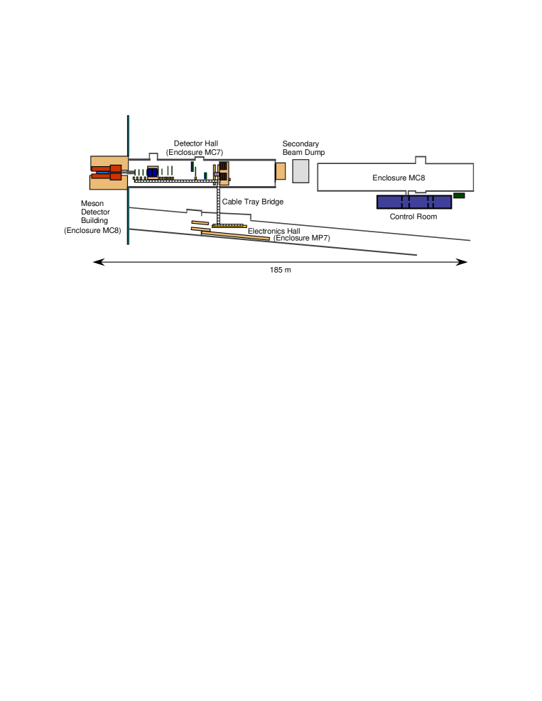
FIGURE 1:

FIGURE 2:

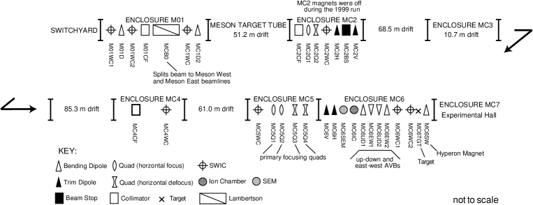
FIGURE 3:

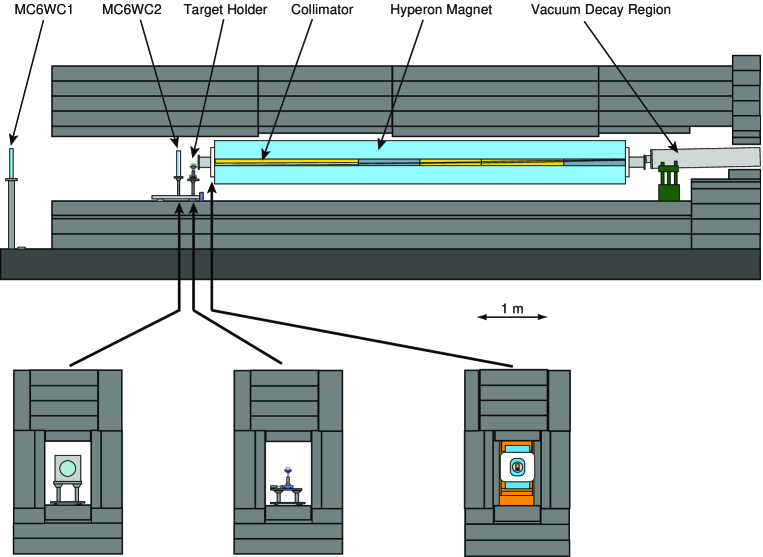
FIGURE 4:

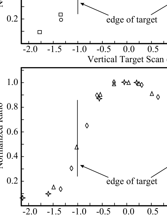
FIGURE 5:

FIGURE 6:

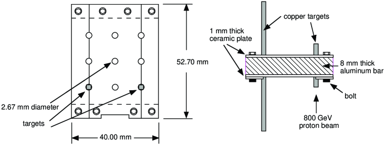
FIGURE 7:

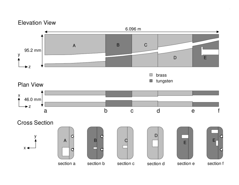
FIGURE 8:

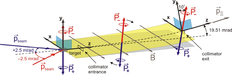
FIGURE 9:

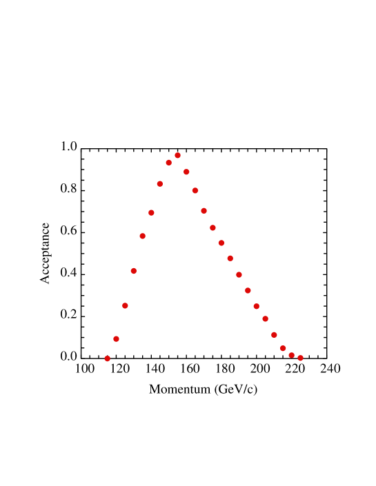
FIGURE 10:

FIGURE 11:

FIGURE 12:

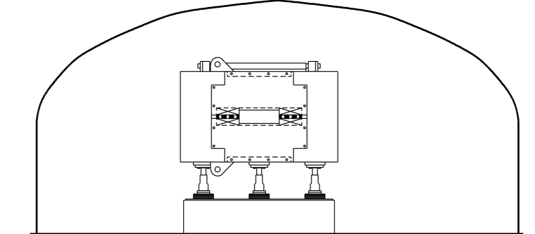
FIGURE 13:

FIGURE 14:

FIGURE 15:

FIGURE 16:

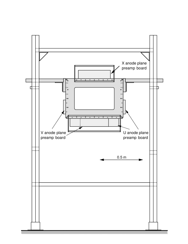
FIGURE 17:

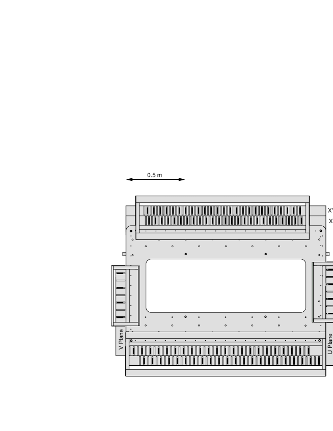
FIGURE 18:

FIGURE 19:

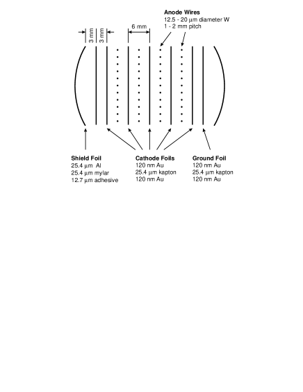
FIGURE 20:

FIGURE 21:

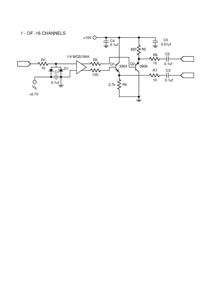
FIGURE 22:

FIGURE 23:

FIGURE 24:

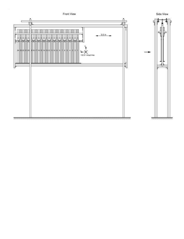
FIGURE 25:

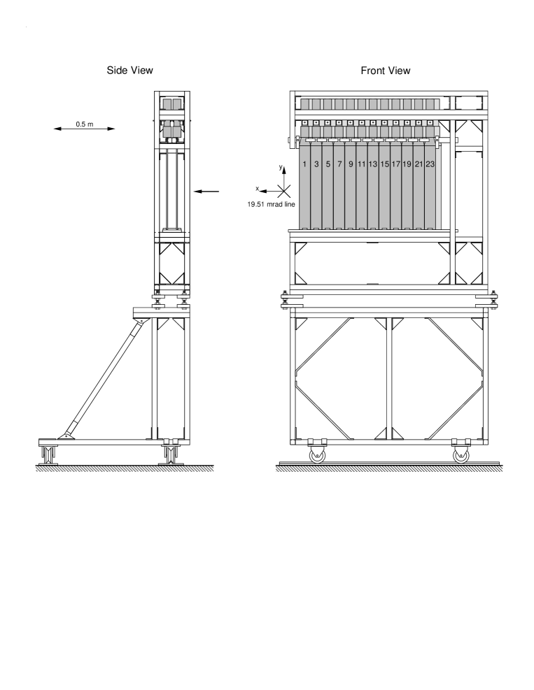
FIGURE 26:

FIGURE 27:

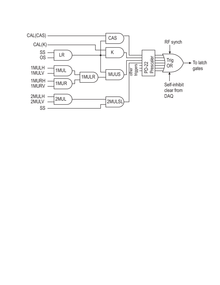
FIGURE 28:

FIGURE 29:

FIGURE 30:

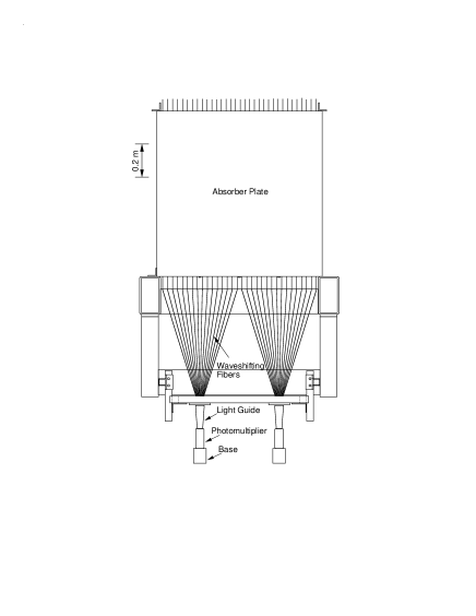
FIGURE 31:

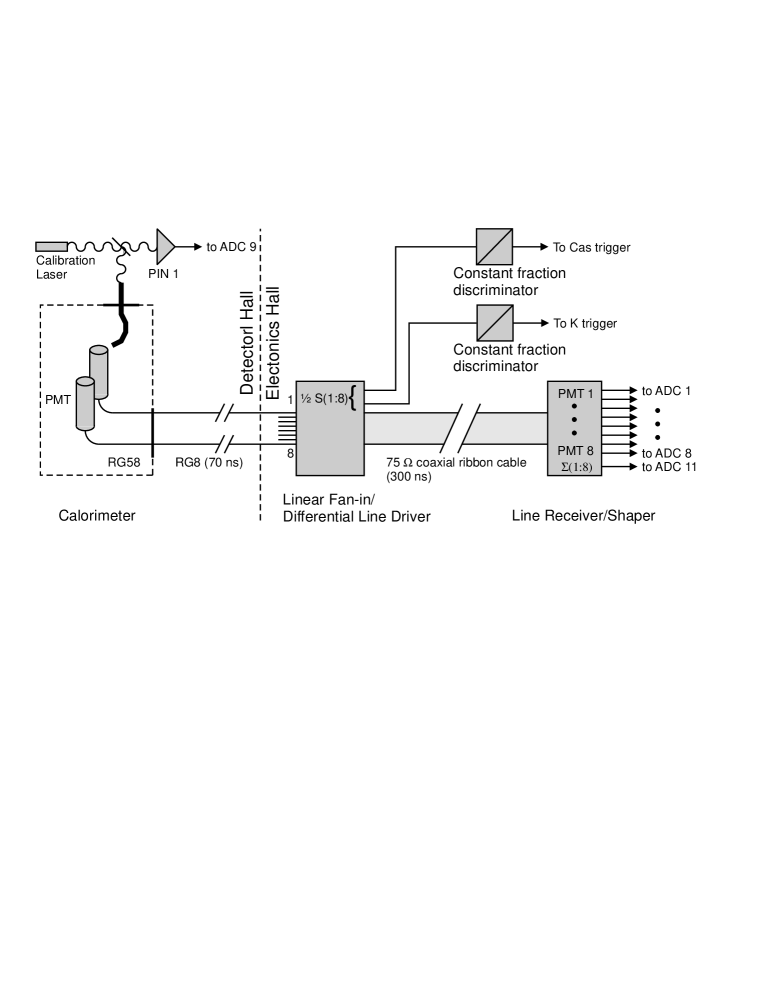
FIGURE 32:

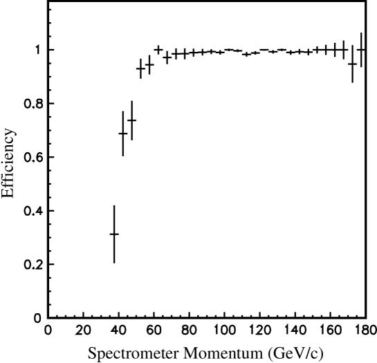
FIGURE 33:

FIGURE 34:

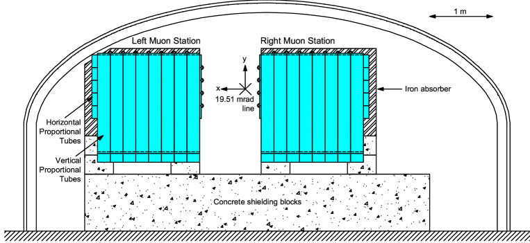
FIGURE 35:

FIGURE 36:

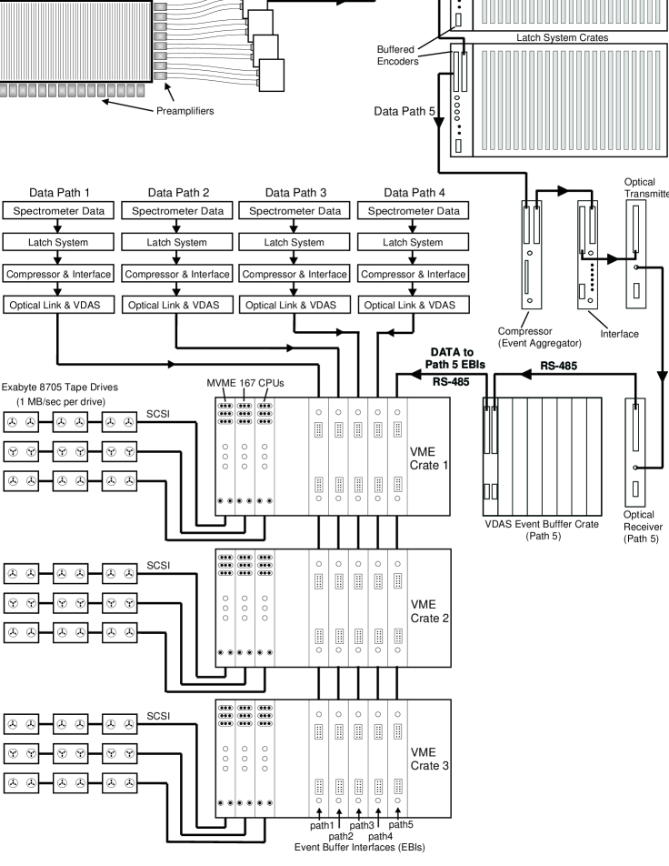
FIGURE 37:

FIGURE 38:

FIGURE 39:

FIGURE 40:

FIGURE 41:

FIGURE 42:

FIGURE 43:

FIGURE 44:

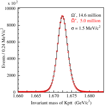
FIGURE 45:

References

- [1] N. Cabibbo, Phys. Rev. Lett. 10, 531 (1963); M. Kobayashi and T. Maskawa, Prog. Theor. Phys. 49, 652 (1973).
- [2] See for example, X.-G. He, H. Murayama, S. Pakvasa, and G. Valencia, Phys. Rev. D 61, 071701(R) (2000).
- [3] K.B. Luk et al., Phys. Rev. Lett. 85, 4860 (2000).
- [4] P.D. Barnes et al., Phys. Rev. C 54, 1877 (1996).
- [5] Portakamp Construction, Inc., P.O. Box 7064, Houston, TX 77248-7064, USA.
- [6] Applied Laser Technology, Inc., 14155 SW Brigadoon Ct., Suite B, Beaverton, OR 97005, USA.
- [7] T. Toohig, “Fermilab Magnets, Power Supplies, and Auxiliary Devices: Technical Data,” Fermilab-TM-632, December 5, 1975.
- [8] Group 3 Technology Ltd., P.O. Box 71-111 Rosebank, Auckland 7, New Zealand.
- [9] N. Leros et al., Nucl. Instrum. Methods A387, 88 (1997).
- [10] DuPont Corp., DuPont Building, 1007 Market St., Wilmington, DE 19898, USA.
- [11] “Magnets and Targetry, Users Manual Section 5," Argonne National Laboratory, March 30, 1966.
- [12] A previous version of the Ziptrack system is described in A. Ito et al., “The Ziptrack Manual," Fermilab-TM-1200, July 1983, and E.N. Prabhakar, “The Ziptrack Integrator," Fermilab-TM-1414, Aug. 1986. The version used here incorporated two main improvements: use of a larger, stiffer I-beam and replacement of the flip-coil field probes with Hall probes.
- [13] Unistrut, 35660 Clinton St., Wayne, MI 48184, USA.
- [14] Stesalit AG, Fabrikweg 54, 4234 Zullwil, Switzerland.
- [15] Shell Chemical, 1600 Smith St., Houston, TX 77210, USA.
- [16] R. Openshaw et al., Nucl. Instrum. Methods A307, 298 (1991).
- [17] LeCroy Corp., 700 Chestnut Ridge Rd., Chestnut Ridge, NY 10977, USA.
- [18] Bicron Newbury, 12345 Kinsman Rd., Newbury, OH 44065, USA.
- [19] Dupont Tyvek-1055B (0.15 mm), DuPont Corp., DuPont Building, 1007 Market St., Wilmington, DE 19898, USA.
- [20] Dupont Tedlar-TCC15BL3, PVF film (0.04 mm), DuPont Corp., DuPont Building, 1007 Market St., Wilmington, DE 19898, USA.
- [21] Hamamatsu Corp., 360 Foothill Rd., Box 6910, Bridgewater, NJ 08807, USA.
- [22] Phillips Scientific, 150 Hilltop Rd., Ramsey, NJ 07446, USA.
- [23] Kuraray International Corp, 30th Floor, PanAm Bldg., 200 Park Avenue, NY 10166, USA.
- [24] EP30M3LV, Master Bond Inc., 154 Hobart St., Hackensack, NJ 07601, USA.
- [25] VSL-337ND Nitrogen Laser, Laser Science, Inc., 8E Forge Parkway, Franklin, MA 02038, USA.
- [26] C. Kerns, IEEE Trans. Nucl. Sci. 24, 353 (1977).
- [27] D. Rajaram, “Design and Performance of a High-Rate Photomultiplier Base,” unpublished M.S. thesis, University of Virginia, 1996.
- [28] DATEL ADS-943 ADC, DATEL, Inc., 11 Cabot Blvd., Mansfield, MA 02048, USA.
- [29] R.J. Yarema, “A New Preamplifier for Particle Detectors," Fermilab-TM-1284, Nov. 1984.
- [30] Nanometric Systems Inc., 451 South Boulevard, Oak Park, IL 60302, USA.
- [31] C.G. White et al., Nucl. Instrum. Methods A474, 67 (2001).
- [32] Y.C. Chen et al., Nucl. Instrum. Methods A455, 424 (2000).
- [33] C.G. White et al., IEEE Trans. Nucl. Sci. 49, 568 (2002).
- [34] Original design ca. 1970 by F.W. Sippach, Columbia University Nevis Laboratories, P.O. Box 137, Irvington, NY 10533, USA, updated for fast readout by F.W. Sippach and H. Cunitz, Columbia University Nevis Laboratories, in 1981. The latch card design was updated from ECL II to ECL 10,000 by J.A. Crittenden and D.M. Kaplan in 1984.
- [35] A.E. Baumbaugh et al., IEEE Trans. Nucl. Sci. 33, 903 (1986); K.L. Knickerbocker et al., IEEE Trans. Nucl. Sci. 34, 245 (1987).
- [36] J.T. Meadows et al., FERMILAB-CONF-95-110, presented at 9th Conference on Real-Time Computer Applications in Nuclear, Particle and Plasma Physics, East Lansing, MI, USA, 22–26 May 1995.
- [37] Motorola Computer Group, 2900 S. Diablo Way, Tempe, AZ 85282, USA.
- [38] Exabyte Corp., 1685 38th St., Boulder, CO 80301, USA.
- [39] Silicon Graphics, 1500 Crittenden Ln., Mountain View, CA 94043.
- [40] JORWAY Co., 27 Bond St. Westbury, NY 11950, USA.
- [41] E. Dambik, “RD Controls Software Release 143.3, SAD Services for Remote Acquisition of Epicure Data," Fermilab Programming Note PN0528 (1997).
- [42] Sony Corporation, 7-35 Kitashinagawa 6-chome, Shinagawa-ku, Tokyo 141-0001, Japan.
- [43] S. Boden et al., in Proc. CHEP’01, Int. Conf. on Computing in High Energy and Nucl. Phys. (Sept. 2001), Beijing, China, Science Press 6-11: 266 (2001).
- [44] National Energy Research Scientific Computing Center, http://www.nersc.gov.
- [45] S. Agostinelli, et al., Nucl. Instrum. Methods A506, 250 (2003).
- [46] G. Bunce, Nucl. Instrum. Methods 172, 553 (1980).
- [47] F. James, Comput. Phys. Commun. 79, 111 (1994).