EUROPEAN ORGANIZATION FOR NUCLEAR RESEARCH

CERN-PH-EP/2004-011

24 March 2004

Scaling violations of quark and gluon
jet fragmentation functions 
in e⁺e^- annihilations
at $\mathbf{\sqrt{}}s=$ 91.2 and 183–209 GeV

The OPAL Collaboration

Abstract

Flavour inclusive, udsc and b fragmentation functions in unbiased jets, and flavour inclusive, udsc, b and gluon fragmentation functions in biased jets are measured in e⁺e^- annihilations from data collected at centre-of-mass energies of 91.2, and 183–209 GeV with the OPAL detector at LEP. The unbiased jets are defined by hemispheres of inclusive hadronic events, while the biased jet measurements are based on three-jet events selected with jet algorithms. Several methods are employed to extract the fragmentation functions over a wide range of scales. Possible biases are studied in the results obtained. The fragmentation functions are compared to results from lower energy e⁺e^- experiments and with earlier LEP measurements and are found to be consistent. Scaling violations are observed and are found to be stronger for the fragmentation functions of gluon jets than for those of quarks. The measured fragmentation functions are compared to three recent theoretical next-to-leading order calculations and to the predictions of three Monte Carlo event generators. While the Monte Carlo models are in good agreement with the data, the theoretical predictions fail to describe the full set of results, in particular the b and gluon jet measurements.

(to be submitted to European Physical Journal C)

G. Abbiendi², C. Ainsley⁵, P.F. Åkesson^3,y, G. Alexander²², J. Allison¹⁶, P. Amaral⁹, G. Anagnostou¹, K.J. Anderson⁹, S. Asai²³, D. Axen²⁷, G. Azuelos^18,a, I. Bailey²⁶, E. Barberio^8,p, T. Barillari³², R.J. Barlow¹⁶, R.J. Batley⁵, P. Bechtle²⁵, T. Behnke²⁵, K.W. Bell²⁰, P.J. Bell¹, G. Bella²², A. Bellerive⁶, G. Benelli⁴, S. Bethke³², O. Biebel³¹, O. Boeriu¹⁰, P. Bock¹¹, M. Boutemeur³¹, S. Braibant⁸, L. Brigliadori², R.M. Brown²⁰, K. Buesser²⁵, H.J. Burckhart⁸, S. Campana⁴, R.K. Carnegie⁶, A.A. Carter¹³, J.R. Carter⁵, C.Y. Chang¹⁷, D.G. Charlton¹, C. Ciocca², A. Csilling²⁹, M. Cuffiani², S. Dado²¹, A. De Roeck⁸, E.A. De Wolf^8,s, K. Desch²⁵, B. Dienes³⁰, M. Donkers⁶, J. Dubbert³¹, E. Duchovni²⁴, G. Duckeck³¹, I.P. Duerdoth¹⁶, E. Etzion²², F. Fabbri², L. Feld¹⁰, P. Ferrari⁸, F. Fiedler³¹, I. Fleck¹⁰, M. Ford⁵, A. Frey⁸, P. Gagnon¹², J.W. Gary⁴, G. Gaycken²⁵, C. Geich-Gimbel³, G. Giacomelli², P. Giacomelli², M. Giunta⁴, J. Goldberg²¹, E. Gross²⁴, J. Grunhaus²², M. Gruwé⁸, P.O. Günther³, A. Gupta⁹, C. Hajdu²⁹, M. Hamann²⁵, G.G. Hanson⁴, A. Harel²¹, M. Hauschild⁸, C.M. Hawkes¹, R. Hawkings⁸, R.J. Hemingway⁶, G. Herten¹⁰, R.D. Heuer²⁵, J.C. Hill⁵, K. Hoffman⁹, D. Horváth^29,c, P. Igo-Kemenes¹¹, K. Ishii²³, H. Jeremie¹⁸, P. Jovanovic¹, T.R. Junk^6,i, N. Kanaya²⁶, J. Kanzaki^23,u, D. Karlen²⁶, K. Kawagoe²³, T. Kawamoto²³, R.K. Keeler²⁶, R.G. Kellogg¹⁷, B.W. Kennedy²⁰, S. Kluth³², T. Kobayashi²³, M. Kobel³, S. Komamiya²³, T. Krämer²⁵, P. Krieger^6,l, J. von Krogh¹¹, K. Kruger⁸, T. Kuhl²⁵, M. Kupper²⁴, G.D. Lafferty¹⁶, H. Landsman²¹, D. Lanske¹⁴, J.G. Layter⁴, D. Lellouch²⁴, J. Letts^o, L. Levinson²⁴, J. Lillich¹⁰, S.L. Lloyd¹³, F.K. Loebinger¹⁶, J. Lu^27,w, A. Ludwig³, J. Ludwig¹⁰, W. Mader³, S. Marcellini², A.J. Martin¹³, G. Masetti², T. Mashimo²³, P. Mättig^m, J. McKenna²⁷, R.A. McPherson²⁶, F. Meijers⁸, W. Menges²⁵, F.S. Merritt⁹, H. Mes^6,a, N. Meyer²⁵, A. Michelini², S. Mihara²³, G. Mikenberg²⁴, D.J. Miller¹⁵, S. Moed²¹, W. Mohr¹⁰, T. Mori²³, A. Mutter¹⁰, K. Nagai¹³, I. Nakamura^23,v, H. Nanjo²³, H.A. Neal³³, R. Nisius³², S.W. O’Neale^1,∗, A. Oh⁸, M.J. Oreglia⁹, S. Orito^23,∗, C. Pahl³², G. Pásztor^4,g, J.R. Pater¹⁶, J.E. Pilcher⁹, J. Pinfold²⁸, D.E. Plane⁸, B. Poli², O. Pooth¹⁴, M. Przybycień^8,n, A. Quadt³, K. Rabbertz^8,r, C. Rembser⁸, P. Renkel²⁴, J.M. Roney²⁶, Y. Rozen²¹, K. Runge¹⁰, K. Sachs⁶, T. Saeki²³, E.K.G. Sarkisyan^8,j, A.D. Schaile³¹, O. Schaile³¹, P. Scharff-Hansen⁸, J. Schieck³², T. Schörner-Sadenius^8,z, M. Schröder⁸, M. Schumacher³, W.G. Scott²⁰, R. Seuster^14,f, T.G. Shears^8,h, B.C. Shen⁴, P. Sherwood¹⁵, A. Skuja¹⁷, A.M. Smith⁸, R. Sobie²⁶, S. Söldner-Rembold¹⁵, F. Spano⁹, A. Stahl^3,x, D. Strom¹⁹, R. Ströhmer³¹, S. Tarem²¹, M. Tasevsky^8,s, R. Teuscher⁹, M.A. Thomson⁵, E. Torrence¹⁹, D. Toya²³, P. Tran⁴, I. Trigger⁸, Z. Trócsányi^30,e, E. Tsur²², M.F. Turner-Watson¹, I. Ueda²³, B. Ujvári^30,e, C.F. Vollmer³¹, P. Vannerem¹⁰, R. Vértesi^30,e, M. Verzocchi¹⁷, H. Voss^8,q, J. Vossebeld^8,h, C.P. Ward⁵, D.R. Ward⁵, P.M. Watkins¹, A.T. Watson¹, N.K. Watson¹, P.S. Wells⁸, T. Wengler⁸, N. Wermes³, G.W. Wilson^16,k, J.A. Wilson¹, G. Wolf²⁴, T.R. Wyatt¹⁶, S. Yamashita²³, D. Zer-Zion⁴, L. Zivkovic²⁴

¹School of Physics and Astronomy, University of Birmingham, Birmingham B15 2TT, UK
²Dipartimento di Fisica dell’ Università di Bologna and INFN, I-40126 Bologna, Italy
³Physikalisches Institut, Universität Bonn, D-53115 Bonn, Germany
⁴Department of Physics, University of California, Riverside CA 92521, USA
⁵Cavendish Laboratory, Cambridge CB3 0HE, UK
⁶Ottawa-Carleton Institute for Physics, Department of Physics, Carleton University, Ottawa, Ontario K1S 5B6, Canada
⁸CERN, European Organisation for Nuclear Research, CH-1211 Geneva 23, Switzerland
⁹Enrico Fermi Institute and Department of Physics, University of Chicago, Chicago IL 60637, USA
¹⁰Fakultät für Physik, Albert-Ludwigs-Universität Freiburg, D-79104 Freiburg, Germany
¹¹Physikalisches Institut, Universität Heidelberg, D-69120 Heidelberg, Germany
¹²Indiana University, Department of Physics, Bloomington IN 47405, USA
¹³Queen Mary and Westfield College, University of London, London E1 4NS, UK
¹⁴Technische Hochschule Aachen, III Physikalisches Institut, Sommerfeldstrasse 26-28, D-52056 Aachen, Germany
¹⁵University College London, London WC1E 6BT, UK
¹⁶Department of Physics, Schuster Laboratory, The University, Manchester M13 9PL, UK
¹⁷Department of Physics, University of Maryland, College Park, MD 20742, USA
¹⁸Laboratoire de Physique Nucléaire, Université de Montréal, Montréal, Québec H3C 3J7, Canada
¹⁹University of Oregon, Department of Physics, Eugene OR 97403, USA
²⁰CCLRC Rutherford Appleton Laboratory, Chilton, Didcot, Oxfordshire OX11 0QX, UK
²¹Department of Physics, Technion-Israel Institute of Technology, Haifa 32000, Israel
²²Department of Physics and Astronomy, Tel Aviv University, Tel Aviv 69978, Israel
²³International Centre for Elementary Particle Physics and Department of Physics, University of Tokyo, Tokyo 113-0033, and Kobe University, Kobe 657-8501, Japan
²⁴Particle Physics Department, Weizmann Institute of Science, Rehovot 76100, Israel
²⁵Universität Hamburg/DESY, Institut für Experimentalphysik, Notkestrasse 85, D-22607 Hamburg, Germany
²⁶University of Victoria, Department of Physics, P O Box 3055, Victoria BC V8W 3P6, Canada
²⁷University of British Columbia, Department of Physics, Vancouver BC V6T 1Z1, Canada
²⁸University of Alberta, Department of Physics, Edmonton AB T6G 2J1, Canada
²⁹Research Institute for Particle and Nuclear Physics, H-1525 Budapest, P O Box 49, Hungary
³⁰Institute of Nuclear Research, H-4001 Debrecen, P O Box 51, Hungary
³¹Ludwig-Maximilians-Universität München, Sektion Physik, Am Coulombwall 1, D-85748 Garching, Germany
³²Max-Planck-Institute für Physik, Föhringer Ring 6, D-80805 München, Germany
³³Yale University, Department of Physics, New Haven, CT 06520, USA

^a and at TRIUMF, Vancouver, Canada V6T 2A3
^c and Institute of Nuclear Research, Debrecen, Hungary
^e and Department of Experimental Physics, University of Debrecen, Hungary
^f and MPI München
^g and Research Institute for Particle and Nuclear Physics, Budapest, Hungary
^h now at University of Liverpool, Dept of Physics, Liverpool L69 3BX, U.K.
ⁱ now at Dept. Physics, University of Illinois at Urbana-Champaign, U.S.A.
^j and Manchester University
^k now at University of Kansas, Dept of Physics and Astronomy, Lawrence, KS 66045, U.S.A.
^l now at University of Toronto, Dept of Physics, Toronto, Canada
^m current address Bergische Universität, Wuppertal, Germany
ⁿ now at University of Mining and Metallurgy, Cracow, Poland
^o now at University of California, San Diego, U.S.A.
^p now at The University of Melbourne, Victoria, Australia
^q now at IPHE Université de Lausanne, CH-1015 Lausanne, Switzerland
^r now at IEKP Universität Karlsruhe, Germany
^s now at University of Antwerpen, Physics Department,B-2610 Antwerpen, Belgium; supported by Interuniversity Attraction Poles Programme – Belgian Science Policy
^u and High Energy Accelerator Research Organisation (KEK), Tsukuba, Ibaraki, Japan
^v now at University of Pennsylvania, Philadelphia, Pennsylvania, USA
^w now at TRIUMF, Vancouver, Canada
^x now at DESY Zeuthen
^y now at CERN
^z now at DESY
^∗ Deceased

1 Introduction

Hadron production in high energy collisions can be described by parton showers (successive gluon emissions and splittings), followed by the formation of hadrons which cannot be described perturbatively. Gluon emission, the dominant process in parton showers, is proportional to the colour factor associated with the coupling of the emitted gluon to the emitter. These colour factors are $C_{A}=3$ when the emitter is a gluon and $C_{F}=4/3$ when it is a quark. Consequently, the multiplicity of soft gluons from a gluon source is (asymptotically) 9/4 times higher than from a quark source [1]. The inequality between $C_{A}$ and $C_{F}$ plays a key role in the explanation of the observed differences between quark and gluon jets: compared to quark jets, gluon jets are observed to have larger widths [2], higher multiplicities [2, 3], softer fragmentation functions [2, 4, 5], and stronger scaling violations of the fragmentation functions [5].

The fragmentation function, $D_{a}^{h}(x,Q^{2})$, is defined as the probability that parton $a$, which is produced at short distance, of order $1/Q$, fragments into hadron, $h$, carrying fraction $x$ of the momentum of $a$. In this study, the momentum fraction is defined as $x_{\mathrm{E}}$ $=E_{h}/E_{\mathrm{j}et}$, where $E_{h}$ is the energy of the hadron $h$ and $E_{\mathrm{j}et}$ is the energy of the jet to which it is assigned. The relative softness of the gluon jet fragmentation function is explained in the low $x_{\mathrm{E}}$ region by the higher multiplicity of soft gluons radiated, and in the high $x_{\mathrm{E}}$ region by the fact that the gluon cannot be present as a valence parton inside a produced hadron (first a splitting ${\mathrm{g}\rightarrow q\bar{q}}$ has to occur). The stronger scaling violation is due to the fact that the scale dependence of the gluon jet fragmentation function is dominated by the splitting function $P_{\mathrm{g}\rightarrow gg}\sim C_{A}$, while that of the quark jet is dominated by the splitting function $P_{\mathrm{q}\rightarrow qg}\sim C_{F}$.

Jets in e⁺e^- annihilations are commonly defined using a jet finding algorithm, which is a mathematical prescription for dividing an event into parts associated with individual quarks and gluons. For example, quark and gluon jets are often defined by applying a jet finder to select three-jet ${\mathrm{q}\bar{q}}$g events. Some of the most common algorithms are the Durham [6] and cone [7] jet finders. Different jet finders result in different assignments of particles to jets: thus jets defined using a jet finding algorithm are called biased. In contrast, quark and gluon jets used in theoretical calculations are usually based on inclusive samples of back-to-back ${\mathrm{q}\bar{q}}$ and gg final states rather than three-jet events. A hemisphere of a ${\mathrm{q}\bar{q}}$ event is defined as a quark jet and similarly, a gluon jet is defined by a hemisphere in a gg final state. The hemisphere definition yields a so-called unbiased jet because the jet properties do not depend on the choice of a jet finder. Measurements of unbiased quark jets have been performed at many scales since such jets correspond to hemispheres of inclusive e⁺e${}^{-}\rightarrow$ hadrons events [8, 9, 10]. Direct measurements of unbiased gluon jets are so far available only from the CLEO [11] and OPAL [4, 12] experiments, however. At CLEO, jets originating from radiative $\Upsilon$ decays have energies of only about 5 GeV, which limits their usefulness for jet studies. In [4, 12], unbiased gluon jets were selected using rare events of the type e⁺e${}^{-}\rightarrow$ ${\mathrm{q}\bar{q}g_{incl}}$, in which the object ${\mathrm{g}_{incl}}$, taken to be the gluon jet, is defined by all particles observed in the hemisphere opposite to that containing two b-tagged quark jets. Due to the low probability of such a topology, this method of obtaining unbiased gluon jets is only viable for very high statistics data samples. Recently, the OPAL experiment has measured properties of unbiased gluon jets indirectly. In [13], recent theoretical expressions to account for biases from event selection were used to extract gluon jet properties over a range of jet energies from about 11 to 30 GeV. In [14], the first experimental results based on the so-called jet boost algorithm, a technique to select unbiased gluon jets in e⁺e^- annihilations, were presented for jet energies from 5 to 18 GeV.

Scaling violations of quark and gluon jet fragmentation functions from three-jet events produced in e⁺e^- collisions at a center-of-mass system (c.m.s.) energy of $\sqrt{s}=$ 91.2 GeV, based on the $k_{T}$ jet algorithms Durham [6] and Cambridge [15], were reported in [5]. These scaling violations were found to be consistent with the expectations from the Dokshitzer-Gribov-Lipatov-Altarelli-Parisi (DGLAP) evolution equations [16]. In our study, we present measurements of quark and gluon jet fragmentation functions at $\sqrt{s}=$ 91.2 GeV and $\sqrt{s}=$ 183–209 GeV. The data were collected with the OPAL detector at the LEP e⁺e^- collider at CERN. We measured seven types of fragmentation functions: the udsc, b, gluon and flavour inclusive fragmentation functions in biased jets, and the udsc, b, and flavour inclusive fragmentation functions in unbiased jets. While the two types of flavour inclusive fragmentation functions have been measured many times, data on the other types of fragmentation functions are still rather scarce.

The paper is organised as follows. In Section 2, a brief description of the OPAL detector is given. The samples of data and simulated events used in the analysis are described in Section 3. In Section 4, the event and jet selections are discussed. The analysis procedure, including the methods used to evaluate systematic uncertainties, is presented in Section 5. Section 6 deals with a Monte Carlo (MC) study of the biases introduced by our jet finding procedure. Next-to-leading order (NLO) calculations [17, 18, 19] for fragmentation functions are described in Section 7. In Section 8, we present a comparison of our data to other measurements, to MC predictions, and to the NLO calculations. A summary and conclusions are given in Section 9.

2 The OPAL detector

The OPAL detector is described in detail elsewhere [20]. The tracking system consists of a silicon microvertex detector, an inner vertex chamber, a large volume jet chamber and specialized chambers at the outer radius of the jet chamber which improve the measurements in the $z$-direction. The tracking system covers the region $|\cos\theta|<0.98$ and is enclosed by a solenoidal magnet with an axial field of 0.435 T. Electromagnetic energy is measured by a lead-glass calorimeter located outside the magnet coil, which covers $|\cos\theta|<0.98$.

3 Data and Monte Carlo samples

The present analysis is based on two data samples which will be referred to as the LEP1 and LEP2 samples. The LEP1 data sample contains hadronic Z decay events collected with the OPAL detector between 1993 and 1995 at c.m.s. energies within 250 MeV of the Z peak. The LEP2 data sample contains hadronic events collected with the OPAL detector in the period 1997–2000 at c.m.s. energies in the range 183–209 GeV. All the data were taken with full readout of the $r$-$\phi$ and $z$ coordinates of the silicon microvertex detector which is essential for precise measurements of primary and secondary vertices. The total integrated luminosity in the LEP1 data is 130 pb^-1, while the LEP2 data sample corresponds to a luminosity of 690 pb^-1.

In this study, we work with three types of MC event samples. The detector level samples include full simulation of the detector response [21], the initial-state photon radiation (ISR) and background processes, and contain only those events which pass the same selection cuts as applied to the data. The hadron level samples do not include ISR or detector simulation and allow all particles with lifetimes shorter than 3 $\times 10^{-10}$ s to decay. The parton level samples are formed by final-state partons, i.e. quarks and gluons present at the end of the perturbative shower, and do not include ISR.

Signal MC events for the LEP1 data, of the form e⁺e${}^{-}\rightarrow$ Z $\rightarrow$ ${\mathrm{q}\bar{q}}$(g), are generated using the JETSET 7.4 [22] and HERWIG 6.2 [23] programs with the parameter settings tuned on LEP1 OPAL data described in [24] and [25], respectively. For LEP2 data, the signal e⁺e${}^{-}\rightarrow$ Z${}^{*}/\gamma^{*}\rightarrow$ ${\mathrm{q}\bar{q}}$(g) events are simulated using PYTHIA 6.125 [22, 26] and HERWIG 6.2. For events of this type, PYTHIA is the same as JETSET except for the inclusion of ISR processes. The same parameter settings are used for the LEP2 PYTHIA and HERWIG samples as are used for the LEP1 JETSET and HERWIG samples, respectively. In the JETSET and PYTHIA event generators, the string fragmentation model is implemented, while HERWIG uses the cluster fragmentation model. The initial- and final-state photon radiation for the LEP2 MC samples are performed by interfacing the KK2F program [27] to the main generator programs. In addition to PYTHIA and HERWIG we also use the ARIADNE 4.08 [28] event generator to compare with the final results. For hadronization, the generator is interfaced to the JETSET 7.4 program. The parameter settings used for ARIADNE are documented in [4, 29].

To estimate the background in the LEP2 data, we generate events of the type e⁺e^-$\rightarrow$ 4 fermions. These events, in particular those with four quarks in the final state, constitute the major background in this analysis. The 4-fermion events are generated using the GRC4F 2.1 [30] MC event program. The final states are produced via s-channel or t-channel diagrams and include W⁺W^- and ZZ events. This generator is interfaced to PYTHIA using the same parameter set for the fragmentation and decays as used for the signal events.

The signal as well as the background MC event samples for the LEP2 period are generated at c.m.s. energies of 183, 189, 192, 196, 200, 202, 204, 205, 206, 207 and 208 GeV reflecting the energy distribution in the collected data samples.

4 Event and jet selection

4.1 Selection of hadronic Z and Z$\mathbf{}*/\gamma^{*}$ events

The procedures for identifying hadronic events are discussed in [31]. The selection of the inclusive hadronic event sample in the LEP1 data is based on tracks and electromagnetic clusters. Tracks are required to have at least 40 measured points (of 159 possible) in the jet chamber, to have a momentum greater than 0.15 GeV/$c$, to lie in the region $|\cos\theta|$$\,<\,$0.94, to have a distance of the point of closest approach to the collision point in the $r$-$\phi$ plane, $d_{0}\leq$ 5 cm, and along the $z$ axis, $z_{0}\leq$ 25 cm. Clusters are required to be spread over at least two lead glass blocks and to have an energy greater than 0.10 GeV if they are in the barrel section of the detector ($|\cos\theta|$$\,<\,$0.82) or greater than 0.20 GeV if they are in the endcap section (0.82$\,<\,$$|\cos\theta|$$\,<\,$0.98). A matching algorithm is employed to reduce double counting of energy in cases where tracks point towards electromagnetic clusters. Specifically, the expected calorimeter energy of the associated tracks is subtracted from the cluster energy. If the energy of a cluster is smaller than that expected for the associated tracks, the cluster is not used. Each accepted track and cluster is considered to be a particle. Tracks are assigned the pion mass. Clusters are assigned zero mass since they originate mostly from photons.

To eliminate residual backgrounds, the number of accepted tracks in each event is required to be at least five. To reject events in which a significant number of particles is lost near the beam line direction, the thrust axis of the event, calculated using the particles, is required to satisfy $|\cos(\theta_{\rm thrust})|$$\,<\,$0.90, where $\theta_{\rm thrust}$ is the angle between the thrust and beam axes. The two-photon background (events of the type $\gamma\gamma\rightarrow$ ${\mathrm{q}\bar{q}}$) is reduced by imposing the conditions $E_{\mathrm{v}is}/\sqrt{s}>0.1$ and $|p_{\rm bal}|<0.6$, where $E_{\mathrm{v}is}$ is the total visible energy (i.e. the sum of detected particle energies) and $p_{\rm bal}$ is the momentum sum in the $z$ direction, normalized by $E_{\mathrm{v}is}$. The residual background in the LEP1 data sample from all sources is estimated to be less than 1% [31]. The number of inclusive hadronic events is $2\,387\,227$ (see the first row in Table 1), with the selection efficiency estimated to be 96%.

At c.m.s. energies above the Z resonance, several new sources of background exist. To select hadronic events in the LEP2 data, the same procedure as described for the LEP1 data is used and in addition, we apply the procedure described in [32, 33, 34, 35] to reduce the background as summarized below.

The majority of hadronic events at LEP2 are radiative events in which initial-state radiation reduces the original c.m.s. energy of the hadronic system. To reject such ISR events, we determine the effective c.m.s. energy of the hadronic system, $\sqrt{s^{\prime}}$, following the procedure described in [35] which takes possible multiple photon radiation into account. We require $\sqrt{s}-\sqrt{s^{\prime}}<$ 10 (20) GeV to select inclusive hadronic events for the hemisphere (three-jet) analysis described below. We refer to this procedure as the “invariant mass” selection. For systematic studies, we apply an alternative method based on combining cuts on the visible energy and missing momentum of the event and on the energy of an isolated photon candidate [32]. This procedure is referred to as the “energy balance” selection. Simulated hadronic Z${}^{*}/\gamma^{*}$ events are defined to be radiative if $\sqrt{s_{\mathrm{t}rue}^{\prime}}<\sqrt{s}-1$ GeV, where $\sqrt{s_{\mathrm{t}rue}^{\prime}}$ is the true effective c.m.s. energy. The efficiency for selecting LEP2 non-radiative hadronic events is 73%.

The production of W⁺W^- and ZZ pairs with hadronic or semi-leptonic decays (4-fermion final states) is an additional source of background. This background is reduced by applying a method described in [35]: first each event is forced into a four-jet configuration using the Durham jet finder. In the LEP2 samples, the 4-momenta of all measured particles are boosted into the rest frame of the hadronic system with the effective c.m.s. energy, $\sqrt{s^{\prime}}$, and are then used to find jets. Then an event weight $W_{\mathrm{Q}CD}$ is defined based on calculated QCD matrix elements for the process e⁺e${}^{-}\rightarrow$ ${\mathrm{q}\bar{q}q\bar{q}}$ or ${\mathrm{q}\bar{q}gg}$, with the four parton final state corresponding to the obtained four-jet kinematics [36]. The QCD matrix elements are calculated using the EVENT2 program [37]. A good separation between the Z${}^{*}/\gamma^{*}$ and W⁺W^- or ZZ pair events is achieved by requiring $W_{\mathrm{Q}CD}\geq-0.5$.

The remaining background from e⁺e${}^{-}\rightarrow$ ${\mathrm{\tau}^{+}\tau^{-}}$ and two-photon events is estimated to be about 0.2% [35] and is neglected. The remaining 4-fermion background is subtracted from the data bin-by-bin. The number of the inclusive hadronic events in the LEP2 data sample for the hemisphere (three-jet) analysis is $10\,866$ ($12\,653$) with 11% (14%) 4-fermion background (see the first row in Table 1).

4.2 Jet selection

As explained in the introduction, we employ two definitions of jets. In the inclusive hadronic event samples we use the unbiased jet definition where the jets are defined by particles in hemispheres of the ${\mathrm{q}\bar{q}}$ system. In the three-jet samples, we apply a jet algorithm and thus work with biased jets. Three jet algorithms are used: the Durham [6], Cambridge [15] and cone [7] algorithms. Relatively large differences in the techniques used by the $k_{T}$ and cone jet finders ensure that the jet finder dependence of the results is estimated conservatively. The jet algorithm is forced to resolve three jets in each event. The jet energies and momenta are then recalculated by imposing overall energy-momentum conservation with planar massless kinematics, using the jet directions found by the jet algorithm. The jet energies are given by the relation:

$$E_{i}=\frac{\sqrt{s}\cdot\sin\theta_{j,k}}{\sin\theta_{i,j}+\sin\theta_{j,k}+\sin\theta_{k,i}}$$ (1)

where $\theta_{i,j}$ is the angle between jets $i$ and $j$ and $k$ corresponds to the remaining jet. We note that for the LEP2 detector level jets, the effective c.m.s. energy, $\sqrt{s^{\prime}}$, is used in the above formula. Cuts, given in Table 2, are chosen to ensure that the jets are well contained within the sensitive part of the detector, well separated from each other and that the event is planar. The numbers of LEP1 and LEP2 events passing these selection criteria are shown in the second row of Table 1. The efficiency for selecting non-radiative three-jet LEP2 events is 68%.

All three jet algorithms yield very similar jet angular and energy resolutions, with the Durham algorithm being slightly better than the other two. Therefore, the Durham algorithm is used as the reference, with the cone and Cambridge jet finders used for systematic studies. The jet energy resolution, defined as $(E_{\mathrm{j}et}^{\mathrm{d}etector}-E_{\mathrm{j}et}^{\mathrm{p}arton})/E_{\mathrm{j}et}^{\mathrm{p}arton}$, is found to range from 2% for the most energetic jet to 11% for the least energetic jet. The distribution of the angles between the detector and parton jet axes is found to have an RMS of 0.05 radians for the most energetic jet and 0.16 radians for the least energetic jet. See Section 5.2.1 for an explanation of how the detector and parton level jets are associated with each other.

5 Analysis procedure

In the following, we describe the method we use to determine the quark and gluon jet fragmentation functions. The measured fragmentation function is defined here as the total number of charged particles, $N_{p}$, in bins of $x_{\mathrm{E}}$ and scale $Q$ normalized to the number of jets, $N_{\mathrm{j}et}(Q)$, in the bin of $Q$:

$$\frac{1}{N_{\mathrm{j}et}(Q)}\frac{{\mathrm{d}}N_{p}(x_{\mathrm{E}},Q)}{{\mathrm{d}}x_{\mathrm{E}}}$$ (2)

where $x_{\mathrm{E}}$ is defined in the Introduction.

5.1 Jet scale $\mathbf{Q}_{\mathrm{\mathbf{missing}}jet}$

To measure the scale dependence, it is necessary to specify a scale relevant to the process under study. For inclusive hadronic events, the scale is $\sqrt{s}$. For jets in three-jet events, neither $\sqrt{s}$ nor $E_{\mathrm{j}et}$ is considered to be an appropriate choice of the scale [38]. QCD coherence suggests [39] that the event topology (i.e. the positions of the partons with respect to each other) should also be taken into account. In studies of quark and gluon jet characteristics [5, 38, 40, 41] the transverse momentum-like scale $Q_{\mathrm{j}et}$, of a jet with energy $E_{\mathrm{j}et}$ has been used:

$$Q_{\mathrm{j}et}=E_{\mathrm{j}et}\sin\frac{\vartheta}{2},$$ (3)

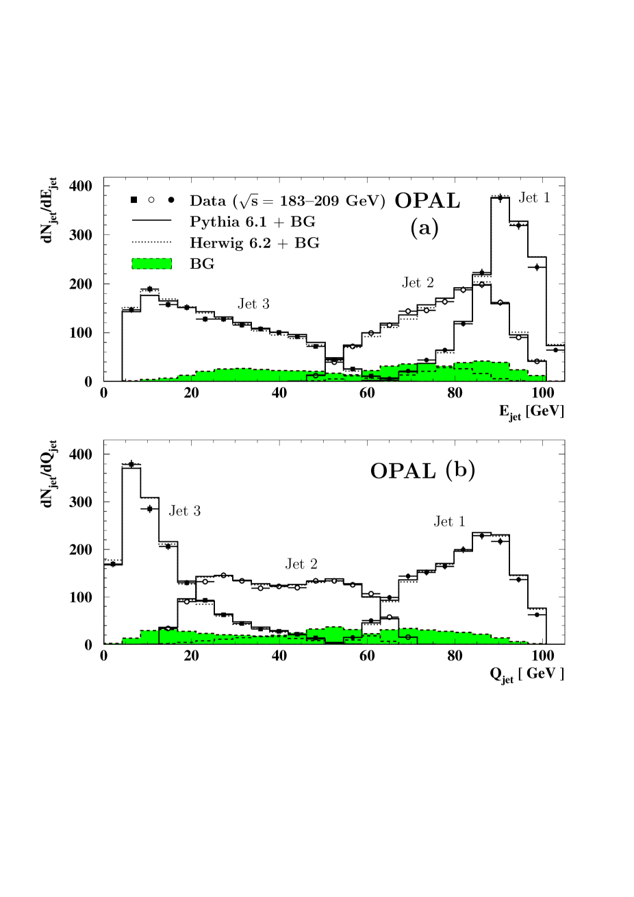
Figure 2: (a) Jet energy and (b) jet scale $Q_{\mathrm{j}et}$ distributions for the selected three-jet events in the LEP2 sample. The solid histograms represent the sum of the PYTHIA 6.125 and background (BG) predictions, the dotted histograms the sum of the HERWIG 6.2 and background predictions and the shaded histograms the prediction of the model GRC4F for the background, all using the Durham jet algorithm. The data are shown with statistical uncertainties only.

where $\vartheta$ is the angle between this jet and the closest other jet. This scale roughly expresses a maximum allowed transverse momentum (or virtuality) of gluons radiated in the showering process with respect to the initial parton, whilst still being associated with the same jet. This definition of scale is adopted for the present analysis. The jet energy and $Q_{\mathrm{j}et}$ spectra are shown in Figs. 1 and 2 for the three jets found by the Durham jet algorithm and ordered in energy, with jet 1 being the most energetic and jet 3 the least energetic jet. The data are seen to be well described by the JETSET and HERWIG models. A similar description is also seen for the cone and Cambridge jet finders (not shown).

5.2 Quark and gluon jet identification

There are several ways to identify quark and gluon jets. In this analysis, three methods are used: the b-tag and the energy-ordering methods to identify quark and gluon jets in biased three-jet events, and the hemisphere method to identify unbiased quark jets in inclusive hadronic events. In addition, b tagging is used to separate udsc and b quark jets from each other, both for the biased and unbiased jet samples. In contrast to the b-tag method, the energy-ordering method only allows flavour inclusive quark jets to be distinguished from gluon jets. Note that the flavour composition of the primary quarks in e⁺e${}^{-}\rightarrow$ ${\mathrm{q}\bar{q}}$ is predicted by electroweak theory to vary with c.m.s. energy. Therefore, to perform a meaningful comparison of the biased jet data taken at $\sqrt{s}=$ 91.2 GeV with the unbiased jet data measured at several c.m.s. energies, a special correction is applied in the construction of the flavour inclusive fragmentation function from biased jets (see Section 5.3).

5.2.1 b-tag method in three-jet events

In the three-jet sample, the b-tagging technique is used to obtain samples enriched in udsc, b or gluon jets. The analysis utilizes an inclusive single jet tag method based on a neural network, as described in [42]. Any or all of the three jets may be used to extract the fragmentation functions. Note that with our selection of three-jet events, the highest energy parton jet is predicted to be the gluon jet in 4.8% of the events.

In the data and MC, three samples of jets are selected, each with different fractions originating from udsc-quarks, b-quarks or gluons. We first look for jets with secondary vertices found in cones of radius $R=0.65$ radians from the jet axes. A jet is considered to be a b-tag jet if it contains a secondary vertex with neural network output value, VNN, greater than 0.8 for LEP1 events or 0.65 for LEP2 events. A jet with no secondary vertex, or a vertex with VNN$<$0.5 is considered to be an “anti-tag” jet. The b-tag and gluon jet samples are taken from events with one or two b-tag jets and at least one anti-tag jet. If one or two b-tag jets and one anti-tag jet are found, the b-tag jets enter the b-tag jet sample and the anti-tag jet enters the gluon jet sample. If one b-tag jet and two anti-tag jets are found, the b-tag jet enters the b-tag jet sample, and the lower energy other jet is included in the gluon jet sample. The udsc jet sample is formed by all three jets in events with no b-tag jet or with b-tag jets but no anti-tag jet (the contribution from the latter events is negligible in practice). Note that with this definition, the gluon jet is explicitly included in the udsc jet sample. The correction procedure to obtain a pure udsc jet sample with the gluon jet component removed is described below.

The purities of the different jet samples are evaluated by examining Monte Carlo events at the parton, hadron and detector levels. First, parton level jets are examined to determine whether they originate from a quark or a gluon. This determination is performed in two ways:

• Flavour assignment: It is assumed that the highest momentum quark and antiquark with the correct flavour for the event are the primary quark and antiquark. In events in which different parton level jets contain the primary quark and antiquark, the remaining jet is assumed to arise from a gluon.

• Non-flavour assignment: A parton jet is identified as a quark (antiquark) jet if it contains an arbitrary number of ${\mathrm{q}\bar{q}}$ pairs and gluons plus one unpaired quark (antiquark). If such two parton jets are found, the gluon jet is defined as that containing only ${\mathrm{q}\bar{q}}$ pairs (if any) and gluons.

A small fraction of events showing an ambiguous assignment of the primary ${\mathrm{q}\bar{q}}$ pair and gluon to three parton level jets is excluded from the event samples. It amounts to 1.3% for the flavour and 2.5% for the non-flavour assignment. To obtain the final results, the former method is used.

Detector and parton level jets are assigned to the hadron jet to which they are nearest in angle. For events in which more than one parton or detector level jets are assigned to the same hadron level jet (about 9% of the events), the closest jet is chosen, while the more distant jet is assigned to the remaining hadron jet. The above procedure is referred to as the “matching” procedure, and the hadron level jets associated with the parton level quark and anti-quark jets are defined to be pure quark jets, while the remaining jet is a pure gluon jet.

The purity and the efficiency of the LEP1 and LEP2 b-tag jet samples as a function of the VNN variable are shown in Fig. 3. The purity of the b-tag jet sample at the point VNN=X is defined as the fraction of pure b jets in the sample of b-tag jets with VNN$>$X. The efficiency of the b-tag jet sample at the point VNN=X is defined as the fraction of the b-tag jets with VNN$>$X in the sample of all pure b jets. For VNN$>$0.8 applied in the LEP1 samples, the purity of the b-tag jet sample is 90% and the efficiency 23%. The corresponding gluon jet purity and efficiency are 84% and 40%, respectively. The LEP2 samples are treated analogously to the LEP1 samples, except that we require VNN$>$0.65 because of low event statistics. The b (gluon) jet tagging efficiency is 27% (45%) and the purity 60% (80%).

To obtain a distribution of a variable $D$ (e.g. the fragmentation function) of pure udsc (b, gluon) jets, $D_{\mathrm{l}(b,g)}^{\mathrm{p}ure}$, one has to solve the following equation

$$\stackrel{{\scriptstyle\mathrm{\ }\ \ \ \ uncor}}{{\left(\begin{array}[]{l}D_{\mathrm{l}}\\ D_{\mathrm{b}}\\ D_{\mathrm{g}}\end{array}\right)\!(x_{\mathrm{E}},Q)}}\ \ =\ \ \left(\begin{array}[]{lll}P_{\mathrm{l}l}~{}\>P_{\mathrm{l}b}~{}\>P_{\mathrm{l}g}\\ P_{\mathrm{b}l}~{}P_{\mathrm{b}b}~{}P_{\mathrm{b}g}\\ P_{\mathrm{g}l}~{}\,P_{\mathrm{g}b}~{}P_{\mathrm{g}g}\end{array}\right)\!(Q)\!\stackrel{{\scriptstyle\mathrm{\ }\ \ \ pure}}{{\left(\begin{array}[]{l}D_{\mathrm{l}}\\ D_{\mathrm{b}}\\ D_{\mathrm{g}}\end{array}\right)\!(x_{\mathrm{E}},Q)}}\\$$ (4)

where $D_{\mathrm{l}(b,g)}^{{}^{\mathrm{u}ncor}}$ stands for a distribution of the variable $D$ obtained from the sample of detector level udsc (b-tag, gluon) jets. The purity $P_{ij}$ denotes the probability that a jet from the jet sample i comes from a parton j. The indices i, j run over symbols l,b and g which stand for the u,d,s,c (“light”)-quark, b-quark and gluon.

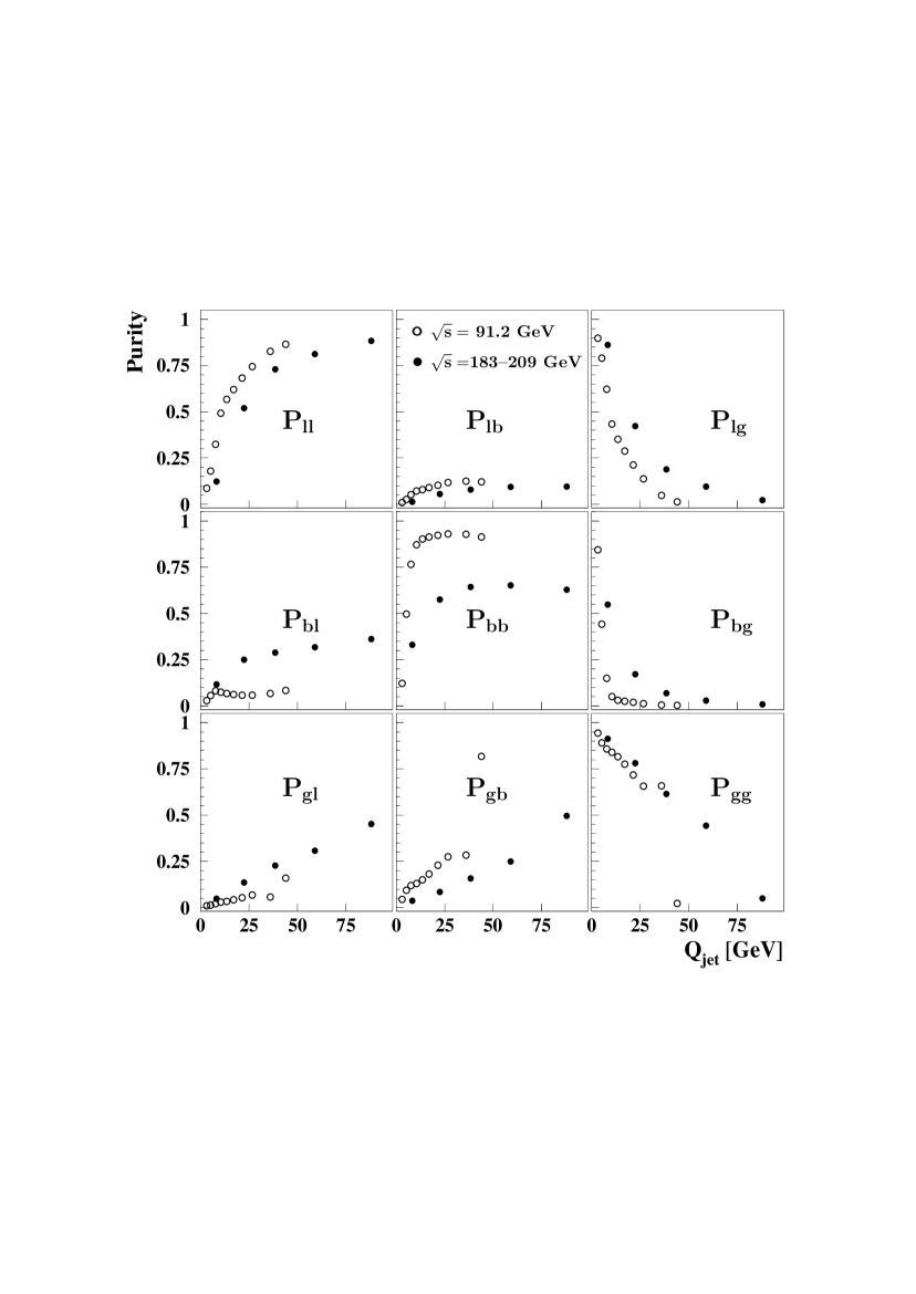
Figure 4: The purity matrix as a function of $Q_{\mathrm{j}et}$ scale for the LEP1 (open circles) and the LEP2 (solid circles) three-jet events, obtained from the JETSET 7.4 for the LEP1 events and PYTHIA 6.125 for the LEP2 events using the Durham jet algorithm. The flavour assignment is used for matching the primary outgoing partons to hadron jets (see text).

In Fig. 4 the LEP1 and LEP2 purity matrices as functions of $Q_{\mathrm{j}et}$ are shown as obtained using the Durham jet algorithm. The numbers of selected udsc, b-tag and gluon jets are shown in Table 1. The larger number of b-tag jets compared to gluon jets is due to the inclusive single jet tag method which allows up to two b-tag jets per event.

5.2.2 Energy-ordering method

This method is based on the QCD prediction that in a three-jet event the lowest energy jet has the highest probability to arise from a gluon. In this method only jets 2 and 3 are used, which form the quark and gluon jet samples, respectively. There are two ways of estimating the purities: either via the matching which employs the inter-jet angles as described in the b-tag method, or using matrix elements. It has been shown [43] that, for leading order QCD matrix elements, the probability for a given jet $i$ among the jets {$i,j,k$} to be a gluon jet can be expressed as a function of the jet energies:

$$P_{i{\mathrm{g}}}\propto\frac{x_{j}^{2}+x_{k}^{2}}{(1-x_{j})(1-x_{k})}$$ (5)

where $x_{i}=2E_{{\mathrm{j}et},i}/\sqrt{s}$. The corresponding probability for the jet to be a quark jet is

$$P_{i\mathrm{q}}=1-P_{i\mathrm{g}},$$ (6)

normalised such that $P_{1\mathrm{q}}+P_{2\mathrm{q}}+P_{3\mathrm{q}}=2$. Thus, in this way, the purities can be obtained based on the kinematics of the data, without recourse to MC information. The scale dependence of the quark purities of jets 1 and 2, and the gluon purity of the jet 3, are shown in Fig. 5. Good agreement is obtained between the data and MC for the matrix element method. The MC results based on matching are seen to agree well with the results based on the matrix elements. For consistency reasons, the purities based on the matching are used to obtain the final results.

An unfolding to the level of pure quark and gluon jets is carried out by solving the following equation:

$$\stackrel{{\scriptstyle\mathrm{\ }\ \ \ \ uncor}}{{\left(\begin{array}[]{l}D_{2}\\ D_{3}\end{array}\right)\!(x_{\mathrm{E}},Q)}}\ \ =\ \ \left(\begin{array}[]{lll}P_{\mathrm{2}q}~{}\>P_{\mathrm{2}g}\\ P_{\mathrm{3}q}~{}\>P_{\mathrm{3}g}\end{array}\right)\!(Q)\!\stackrel{{\scriptstyle\mathrm{\ }\ \ \ pure}}{{\left(\begin{array}[]{l}D_{\mathrm{q}}\\ D_{\mathrm{g}}\end{array}\right)\!(x_{\mathrm{E}},Q)}}\\$$ (7)

where $D_{2(3)}^{\mathrm{u}ncor}$ is the detector level distribution of a variable $D$ in the sample of jets 2 (3) and $D_{\mathrm{q}(g)}^{\mathrm{p}ure}$ corresponds to pure quark (gluon) jets. The energy-ordering method can only be applied in the $Q_{\mathrm{j}et}$ region where the samples of jets 2 and 3 overlap ($6<Q_{\mathrm{j}et}<$ 27 GeV for the LEP1 and $10<Q_{\mathrm{j}et}<$ 60 GeV for the LEP2 sample).

5.2.3 Hemisphere method

In the inclusive hadronic event sample we again use b-tagging to obtain samples enriched in b and udsc jets. In the LEP1 sample, a b-tag event is defined by requiring two secondary vertices with VNN$>$0.8, while in the LEP2 sample—due to limited statistics—only one secondary vertex with VNN$>$0.8 is required. All remaining events form the udsc event sample. Events with no requirement on the presence of a secondary vertex form the inclusive hadronic event sample. Each event contains two unbiased jets (hemispheres) of the same energy, $\sqrt{s}/2$. The jets are unfolded to the level of pure udsc and b jets using an analogous procedure to that described in Section 5.2.2 for the energy-ordering method. In Eq. (7), we replace the indices 2 and q by the index l, and the indices 3 and g by the index b. The purity $P_{\mathrm{b}l}$ ($P_{\mathrm{l}l}$) then denotes the probability that a jet from the b-tag (udsc) jet sample comes from an u,d,s or c-quark. In the LEP1 MC sample, $P_{\mathrm{l}l}=$79% and $P_{\mathrm{b}b}=$99.7% which means that we work with a very pure b-tag jet sample. The corresponding purities for the LEP2 MC sample are 89% and 75%. The numbers of unbiased udsc and b-tag jets passing the selection cuts together with background estimates (for the LEP2 data) are summarized in Table 1. The higher efficiency of selecting non-ISR events and the lower background compared to those for the biased jets is due to the tightened cut on the c.m.s. energy described in Section 4.1.

5.3 Construction of flavour inclusive fragmentation function from
biased jets

To construct the flavour inclusive fragmentation function from the LEP1 biased jets, the samples of udsc, b-tag and gluon jets from the b-tag method are used. The quark jet sample is formed by a sum of the udsc and b-tag jet samples. The unfolding to the level of pure quark and gluon jets can then proceed by use of Eq. (7) where the sample of jets 2 is replaced by the quark jet sample and the sample of jets 3 by the gluon jet sample. To take into account the $\sqrt{s}$ dependence of the flavour composition of the primary ${\mathrm{q}\bar{q}}$ pair, the sample of pure quark jets is constructed as a sum of samples of pure udsc and b jets, weighted by factors of $r_{\rm udsc}(\langle Q_{\mathrm{j}et}\rangle)$ and $r_{\mathrm{b}}(\langle Q_{\mathrm{j}et}\rangle)$, respectively. The $r_{\mathrm{b}}(\langle Q_{\mathrm{j}et}\rangle)$ factor is calculated using the hadron level MC, as the ratio of the b$\bar{\mathrm{b}}$ production rate for a given $Q_{\mathrm{j}et}$ bin with a mean value of $\langle Q_{\mathrm{j}et}\rangle$ in three-jet events generated at $\sqrt{s}=$ 91.2 GeV and the b$\bar{\mathrm{b}}$ production rate in inclusive hadronic events generated at $\sqrt{s}=\langle Q_{\mathrm{j}et}\rangle$. The factor $r_{\rm udsc}(\langle Q_{\mathrm{j}et}\rangle)$ is determined in an analogous fashion. The corrections based on $r_{\mathrm{b}}$ and $r_{\rm udsc}$ are smaller than 15% and bring the biased jet data closer to the published unbiased jet data.

5.4 Correction procedure

The remaining 4-fermion background in the LEP2 data is estimated for each observable by MC simulation and subtracted on a bin-by-bin basis from the data distributions, as already mentioned in Section 4.1. Then the data and MC distributions at the detector level are corrected to the level of pure quarks and gluons by solving either Eq. (4) or Eq. (7). As a last step, we correct the data for the effects of limited detector acceptance and resolution as well as for the presence of remaining radiative events. The data are multiplied, bin-by-bin, by correction factors calculated as ratios of distributions at the hadron level to those at the detector level. For the hadron level biased jets, the same jet selection criteria as described in Section 4.2 are applied except that the jets are not required to satisfy $|\cos\theta_{\mathrm{j}et}|\leq 0.90$. The quark and gluon jets at the hadron level are identified with MC information using the matching technique described in Section 5.2.1. The correction factors from JETSET/PYTHIA used to correct the data do not exceed 20%. The correction factors from HERWIG used to estimate the model dependence of the results are similar. A bin-by-bin correction procedure is suitable for the measured distributions as the detector and ISR effects do not cause significant migration (and therefore correlation) between bins. Typical bin purities for the $Q_{\mathrm{j}et}$ binning chosen were found to be 75%, the lowest value was 65%.

5.5 Systematic uncertainties

The systematic uncertainties of the measurements are assessed by repeating the analysis with the following variations to the standard analysis.

1. The systematics on the modelling of the Z and Z${}^{*}/\gamma^{*}$ events used to correct the data for ISR, detector effects and quark and gluon jet misidentification is estimated by using HERWIG instead of JETSET/PYTHIA. In the bulk of the measured data, the maximum differences for all types of fragmentation functions do not exceed 6%. In the last $x_{\mathrm{E}}$ bin of both types of flavour inclusive fragmentation functions ($0.8<x_{\mathrm{E}}<1.0$), the two models deviate from each other by as much as 50–60%.

2. To assess any inadequacies in the simulation of the response of the detector in the endcap regions, the analysis was restricted to the barrel region of the detector, requiring the tracks and electromagnetic clusters to lie within the range $|\cos\theta_{\mathrm{p}article}|<0.70$. The maximum differences reach 10% for biased jets (for large $x_{\mathrm{E}}$) and 2% for unbiased jets.

3. Potential sensitivity of the results to details of the track selection is assessed by repeating the analysis with modified track selection criteria: the maximum allowed distance of the point of closest approach of a track to the collision point in the $r-\phi$ plane, $d_{0}$, is changed from 5 to 2 cm, the maximal distance in the $z$ direction, $z_{0}$, from 25 to 10 cm and the minimal number of hits from 40 to 80. The quadratic sum over the deviations from the standard result, obtained from each of these variations, is included to the total systematic uncertainty. In most of the bins, the changes are below 1%. Larger changes are observed for high $x_{\mathrm{E}}$, where they are within 7% for both, the biased and unbiased jets.

4. The jet algorithm dependence of the biased jet results is estimated by repeating the analysis using Cambridge and cone jet algorithms. The largest of the two deviations from the standard result (the cone algorithm in most of the bins) is taken as the systematic uncertainty. All differences are within 10% for all types of fragmentation functions, except at low $Q_{\mathrm{j}et}$ and $x_{\mathrm{E}}$ ($4<Q_{\mathrm{j}et}<9$ GeV with $0.02<x_{\mathrm{E}}<0.04$) where the results of the cone algorithm are about 20%, 24%, 31% and 36% below the results of the Durham algorithm, for the flavour inclusive, udsc, b and gluon jet fragmentation function, respectively. The differences between the results for individual jet algorithms diminish with increasing jet energy.

5. The jet selection criteria were varied. The minimum particle multiplicity per jet is changed from 2 to 4; the minimum corrected jet energy is changed from 5 GeV to 3 and 7 GeV; the minimum inter-jet angle is changed from 30^∘ to 25^∘ and 35^∘ and the minimum sum of inter-jet angles is changed from 358^∘ to 356^∘ and 359^∘. The largest deviation with respect to the standard result is taken as the systematic uncertainty. The differences are below 2% in all cases, except for large $x_{\mathrm{E}}$ with small $Q_{\mathrm{j}et}$ where they reach 6%.

6. The dependence of the results on the neural network output value is estimated by varying the cut on VNN from 0.50 to 0.95. The maximum of the deviations with respect to the standard result is taken as the systematic uncertainty. Typical deviations are 2% for unbiased jets and the LEP1 biased jets, while they are 5% for the LEP2 biased jets. The largest deviation is 11% for the unbiased jets and 20% for the biased jets (both observed for large $x_{\mathrm{E}}$).

7. The b-tagging efficiency is determined using MC events. The systematic uncertainty in this efficiency was estimated to be about 5% for VNN$>$0.50 in LEP2 data [44]. The effect of this uncertainty is assessed by changing the VNN thresholds in the MC samples such that the b-tagging efficiency increases or decreases by 10%, while leaving the thresholds in the data unchanged. The largest deviation with respect to the standard result is taken as the systematic uncertainty. In most of the bins, the differences are below 1%. In the high $x_{\mathrm{E}}$ region, they reach 4% for unbiased jets and are typically within 8% for biased jets.

8. The uncertainty in the estimates of purities for the b-tag method is accounted for by using the non-flavour assignment instead of the flavour assignment of the outgoing primary ${\mathrm{q}\bar{q}}$ pair and gluon to three parton jets. Non-negligible differences in the purities are seen only in those $Q_{\mathrm{j}et}$ regions where the purities are small. This results in negligible effects on the final results: they are below 1% everywhere. In case of the energy-ordering method, the procedure based on the matrix elements is used instead of the matching. The differences for the gluon jet fragmentation functions are below 1% everywhere.

9. Uncertainties arising from the selection of non-radiative LEP2 events are estimated by using the “energy balance” procedure instead of the “invariant mass” procedure. The differences are below 5% for both the biased and unbiased jets.

10. Systematic uncertainties associated with the subtraction of the 4-fermion background events in the LEP2 samples are estimated by varying the cut on $W_{\mathrm{Q}CD}$ from -0.5 to 0.0 and -0.8. The maximum of the deviations with respect to the standard result is taken as the systematic uncertainty. The differences are below 4% for both the biased and unbiased jets. In addition, we varied the predicted background to be subtracted by $\pm$5%, slightly more than its measured uncertainty at $\sqrt{s}=189$ GeV of 4% [45]. The differences are below 1% everywhere.

The results for the udsc jets are found to be less sensitive to the above variations than the results for b and gluon jets. The largest changes in the numbers of selected b and gluon jets relative to those shown in Table 1 are given by variation 6. For the LEP1 sample, the number of b-tag (gluon) jets grows by 55% (44%) for VNN=0.5 and drops by 40% (37%) for VNN=0.95. Variation 6 also gives rise to the most significant change in the purities of the b-tag and gluon jet samples. The b (gluon) purity decreases by 17% (5%) for VNN=0.5, while it increases by 7% (2%) for VNN=0.95 (the b-purity shown in Fig. 3a). Other variations change the purities very little.

The differences between the standard results and those found using each of the above conditions are used to define symmetric systematic uncertainties. To reduce the influence of statistical fluctuations, the systematic uncertainties from all sources are determined for a few larger $Q_{\mathrm{j}et}$ bins, each of them exactly covering two or three original bins. The systematic deviation found for this larger bin is then assigned to all original bins contained in it. The total systematic uncertainty is defined as the quadratic sum of these deviations.

6 Monte Carlo comparison of biased and unbiased jets

As discussed above, jets found using a jet algorithm are biased and in this sense are less suitable for comparison with theory than unbiased jets. To assess the difference between biased and unbiased jets, we perform a comparison of their properties using hadron level MC event samples. For this purpose, we choose HERWIG because it contains an event generator for gg events from a colour singlet point source and because it describes well gluon jet properties [4].

The conclusions from the comparison of the biased and unbiased jet fragmentation functions are basically independent of the Monte Carlo model and jet algorithm used in the analysis, therefore, as an example, we show in Fig. 6 the comparison for HERWIG 6.2 and the Durham jet algorithm. The results correspond to the hadron level described in Section 5.4. The three-jet events (i.e. containing biased jets) are generated at $\sqrt{s}=$ 91.2 GeV. The inclusive hadronic events (no jet finder used, so containing unbiased jets) are generated separately at values of $\sqrt{s}$ corresponding to twice the central values of $Q_{\mathrm{j}et}$ in the individual $Q_{\mathrm{j}et}$ intervals used in the analysis of three-jet events. Differences between biased and unbiased jet properties are expected due to different scales used ($Q_{\mathrm{j}et}$ vs. $\sqrt{s}/2$) and different number of jets per event (two hemispheres vs. three jets found by a jet algorithm and spatially restricted by the minimum inter-jet angle of 30^∘). We point out four regions of phase space where the differences between the biased and unbiased jet fragmentation functions are larger than 15%:

a) Small scales with small $x_{\mathrm{E}}$ for all fragmentation functions: This difference, which decreases with increasing scale and $x_{\mathrm{E}}$, may in part be explained by hadron mass effect. At small c.m.s. energies, hadron masses are not negligible with respect to jet energies, causing a suppression of the fragmentation functions at very low $x_{\mathrm{E}}$. This effect is not present in theory (hadrons are taken to be massless) and is less strong in three-jet events (the mean value of $E_{\mathrm{j}et}$ in the first $Q_{\mathrm{j}et}$ bin is about 13 GeV) so one can expect the three-jet data to be better described by theory than the unbiased jet data in these bins.

b) Small scales with large $x_{\mathrm{E}}$ for b jet fragmentation functions: Since this difference increases with increasing $x_{\mathrm{E}}$ and decreasing scale, it might be explained by the b-quark mass effect, i.e. by the ratio $m_{\mathrm{b}}/E_{\mathrm{j}et}$. At small c.m.s. energies, just above the ${\mathrm{b}\bar{b}}$ production threshold ($\sqrt{s}=2m_{\mathrm{b}}\approx 10$ GeV), the above ratio is close to 100% and almost all particles picked up in the hemispheres come from decays of B hadrons, resulting in a very small probability to produce a particle with $x_{\mathrm{E}}$ close to unity. As the scale increases, there is more and more phase space for gluon showers, leading to more hadrons from the fragmentation process. However, the number of radiated gluons is limited by the so-called “dead cone effect” [46], i.e. by a suppression of the gluon emission within an angle of order $m_{\mathrm{b}}/E_{\mathrm{j}et}$. In three-jet events, the ratio $m_{\mathrm{b}}/E_{\mathrm{j}et}$ starts at a much smaller value than in hemisphere events (since the mean jet energy in the first $Q_{\mathrm{j}et}$ bin is about 13 GeV) leading to much more phase space for gluon showering compared to hemisphere jets with the same value of scale. In QCD calculations based on unbiased jets, this ratio can be identified with mass terms of the type $m_{\mathrm{q}}/Q$ where $Q$ is some hard scale. In current NLO calculations, these mass terms are not considered. As will be seen later, the three-jet data and theory behave similarly in the region of small scales. This similarity suggests that missing mass terms in theory may behave like $m_{\mathrm{b}}/E_{\mathrm{j}et}$.

c) Large $x_{\mathrm{E}}$ for gluon jet fragmentation functions: The sizable discrepancy observed for $x_{\mathrm{E}}>0.6$ clearly suggests a bias in the gluon jet results. It appears to be more appropriate [47] to consider for example both the energy scale and the exact virtuality scale and to boost to a frame in which the two scales are equal. MC studies recently presented by OPAL in [14] demonstrate that such boosted gluon jets are less biased than those from our study, in particular in the regions of very small and large $x_{\mathrm{E}}$.

d) The last scale bin for all quark jet fragmentation functions: The observed difference is larger than 15% in the $x_{\mathrm{E}}$ ranges of 0.01–0.07 and 0.40–0.90. Although biased jets in the interval $44<Q_{\mathrm{j}et}<46$ GeV should in principle resemble hemispheres of the same energy (due to large angles $\vartheta$ reaching up to 165^∘), we found that the soft particle multiplicity differs between the two cases. Therefore this difference is considered to represent a true bias of biased jets.

The comparisons made in this MC study suggest that biased jets are less sensitive to hadron and b-quark mass effects than unbiased jets. This implies that biased jets tend to be more appropriate for comparisons with theory than unbiased jets in the regions of low scale with low $x_{\mathrm{E}}$, and in case of b jets, also at low scale with high $x_{\mathrm{E}}$.

7 NLO predictions

The results are compared to theoretical predictions by three groups, namely Kniehl, Kramer and Pötter (KKP) [17], Kretzer (Kr) [18] and Bourhis, Fontannaz, Guillet and Werlen (BFGW) [19]. The three groups provide numerical values of the quantity defined in Eq. (2), up to the next-to-leading order in $\alpha_{S}$. This means that in the extraction of these predictions from measured charged particle momentum distributions, the hard scattering cross section for the production of a parton in e⁺e^- annihilation is evaluated to an accuracy of the order $\alpha_{S}$, while the splitting functions describing the scale dependence are evaluated to an accuracy of the order $\alpha_{S}^{2}$. We stress that these NLO predictions correspond to an unbiased jet definition. The scale evolution via DGLAP evolution equations is performed starting from fragmentation functions at a fixed input scale, extracted from existing measurements. In each of these calculations, the renormalization and fragmentation scales are set equal to the hard scale $Q$. The calculations, nevertheless, differ in a number of important aspects, such as the choice of data sets, the definition of the scale $Q$, the fit ranges, the prescription for the number of active flavours in the evolution of fragmentation functions and partonic cross sections, and the treatment of heavy flavours and gluons.

More specifically, in [17] the evolution of the b jet fragmentation function starts at scale $Q=2m_{\mathrm{b}}$ where $m_{\mathrm{b}}$ is the b-quark mass put equal to 4.5 GeV. The number of active flavours, $N_{\mathrm{a}ctive}^{f}$, is driven by twice the quark mass, $2m_{\mathrm{q}}$ ($N_{\mathrm{a}ctive}^{f}=4$ for $2m_{\mathrm{c}}<Q<2m_{\mathrm{b}}$ and similarly for other flavours). The QCD scale parameter for five flavours and the $\overline{\mathrm{M}S}$ renormalization scheme, $\Lambda_{\overline{\mathrm{\scriptscriptstyle}MS}}^{\scriptscriptstyle(5)}$, is set equal to 0.213 GeV. In [18] the start of the b jet fragmentation function evolution is at the scale $Q=m_{\mathrm{b}}$, $N_{\mathrm{a}ctive}^{f}$ is driven by $2m_{\mathrm{q}}$ and $\Lambda_{\overline{\mathrm{\scriptscriptstyle}MS}}^{\scriptscriptstyle(5)}=$ 0.168 GeV. In [19] the fragmentation functions are evolved using an “optimal” scale, $Q_{\mathrm{o}pt}$, given by the relation $Q^{2}\frac{\delta D_{a}^{h}}{\delta Q^{2}}\left|{}_{Q=Q_{\mathrm{o}pt}}\right.=0$. The evolution of the b jet fragmentation function starts at scale $Q=m_{\mathrm{b}}$, and $\Lambda_{\overline{\mathrm{\scriptscriptstyle}MS}}^{\scriptscriptstyle(4)}=$0.300 GeV.

The predictions for quark jet fragmentation functions by KKP, Kr and BFGW were made using data from [8, 9, 10, 48] or similar results. Concerning the predictions for gluon jet fragmentation functions, it is important to note that in [17] a fit was made to the unbiased [4] and biased [49] jet data, in [18] the predictions were obtained from the evolution and the NLO correction to the e⁺e^- cross section and in [19] a fit was made to large $p_{T}$ charged particle data [50]. Therefore, the experimental input for gluon jets is very different in the three calculations. The fit ranges used by KKP, Kr and BFGW were $0.1<x_{\mathrm{E}}<1.0$, $0.05<x_{\mathrm{E}}<0.8$ and $0.12<x_{\mathrm{E}}<0.9$, respectively. We obtained the NLO predictions of Kr and BFGW using the code [51] where they are provided in parameterised forms. The relative difference between the parameterisation and the exact evolution for predictions by Kr are smaller than 3% and 10% for $x_{\mathrm{E}}<0.75$ and $x_{\mathrm{E}}<0.90$, respectively. All the NLO curves by KKP shown in this analysis correspond to the exact scale evolution.

We point out that in the NLO predictions, the NLO (of the order $\alpha_{S}$) corrections to the hard subprocess correspond to inclusive hadron production. For three-jet events, NLO corrections are not available and are expected to depend on the jet algorithm used. Our assumption in this analysis is that where the biased jet data are observed to be in a good agreement with the unbiased jet data, the unknown NLO corrections are apparently small, and the biased jet results can be compared to the existing NLO predictions. Despite the sizable differences between the biased and unbiased jet MC results reported in points a) and b) of Section 6, the biased jet data at low scales are still considered to be appropriate for such a comparison for the reasons mentioned at the end of Section 6.

8 Results

In the following, the results from this analysis are compared with existing measurements as well as with various fragmentation models and theoretical NLO predictions. The fragmentation functions are presented either with emphasis on the scale dependence or the $x_{\mathrm{E}}$ dependence. The scale dependent fragmentation functions are plotted in several $x_{\mathrm{E}}$ intervals as functions of scale. For a given bin of scale, the data or MC point is placed at the value of the scale at which the NLO prediction is equal to its mean value over this bin [52]. An analogous prescription is applied for the $x_{\mathrm{E}}$ dependent fragmentation functions. Since in the following, the biased and unbiased jet results are often plotted on the same figure, we have to accommodate the differences between scale definitions and number of jets from which the fragmentation functions were extracted. Therefore the term scale in the following figures stands for $Q_{\mathrm{j}et}$ in case of biased jets and $\sqrt{s}/2$ in case of unbiased jets. The published unbiased jet results are scaled by $\frac{1}{2}$ since they refer to the entire event, thus to two jets. For the NLO predictions, the same prescription as for the published unbiased jet data is applied.

8.1 Scale dependence

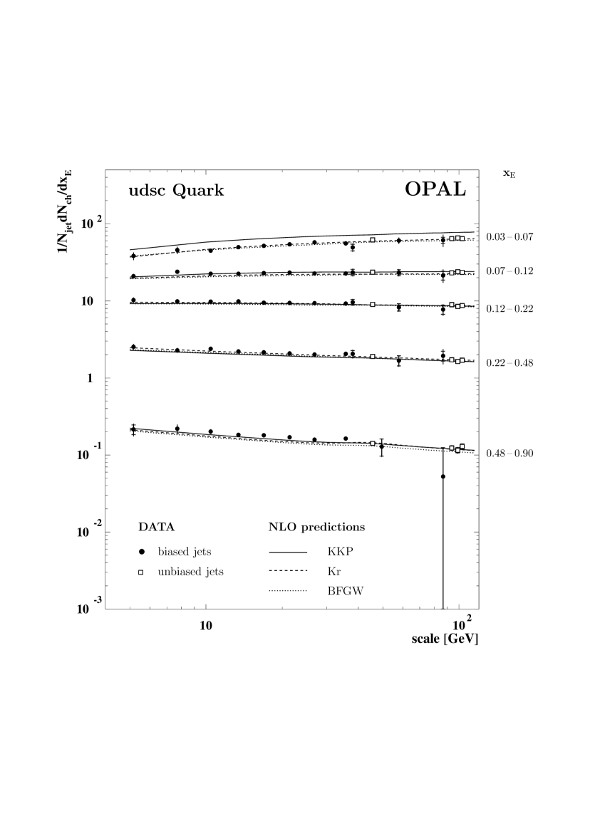
Figure 7: Scale dependence of the udsc jet fragmentation functions in different $x_{\mathrm{E}}$ bins. The scale denotes $Q_{\mathrm{j}et}$ for the biased jets and $\sqrt{s}/2$ for the unbiased jets. The inner error bars indicate the statistical uncertainties, the total error bars show the statistical and systematic uncertainties added in quadrature. The values are given in Table 3. The data are compared to the NLO predictions by KKP [17], Kr [18] and BFGW [19].

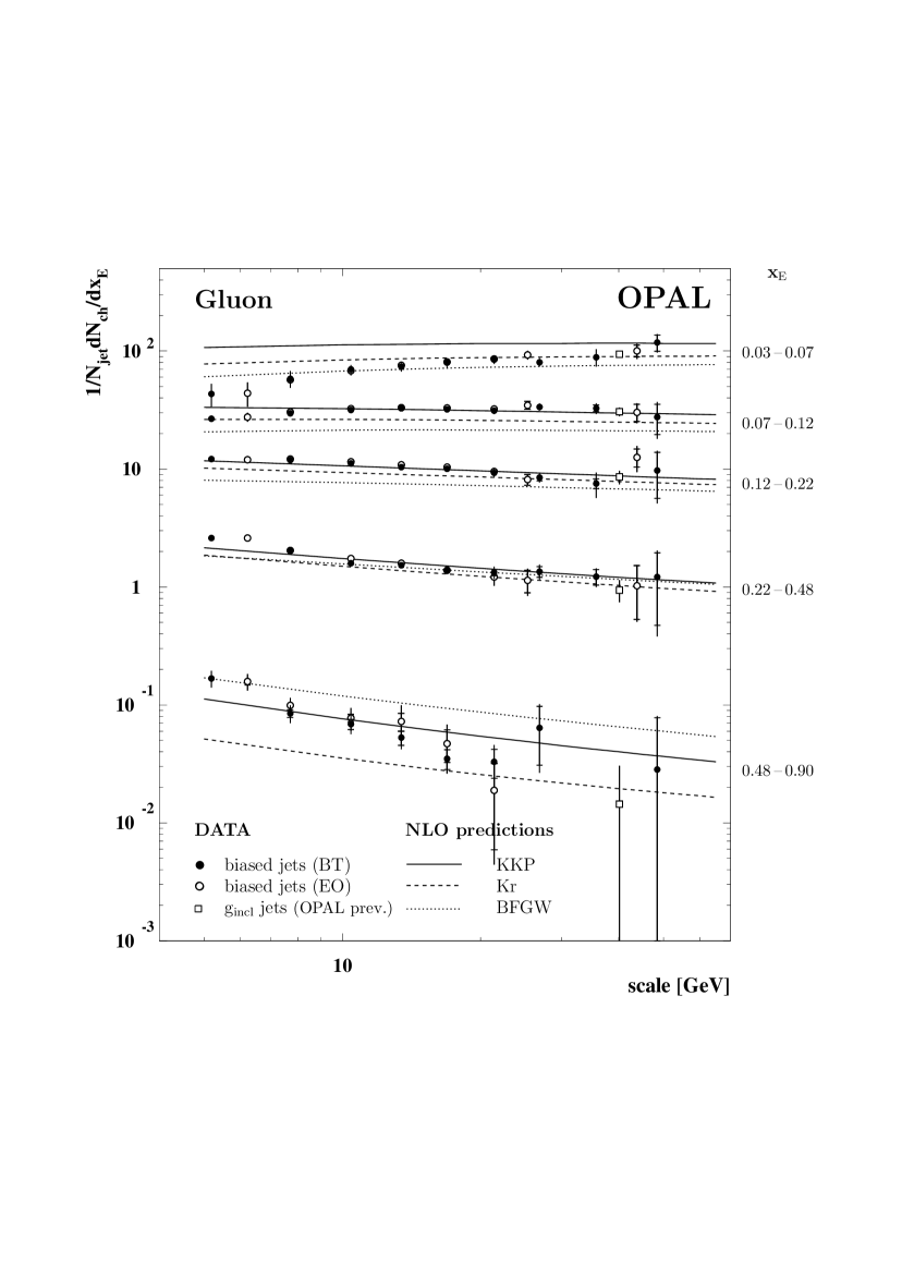
Figure 9: Scale dependence of the gluon jet fragmentation functions in different $x_{\mathrm{E}}$ bins. The scale denotes $Q_{\mathrm{j}et}$ for the biased jets and $E_{\mathrm{j}et}$ for the published ${\mathrm{g}_{incl}}$ jets (OPAL [4]). The results from the biased jets using the b-tag (BT) and the energy-ordering method (EO) are shown. The inner error bars indicate the statistical uncertainties, the total error bars show the statistical and systematic uncertainties added in quadrature. The values are given in Table 5. The data are compared to the NLO predictions by KKP [17], Kr [18] and BFGW [19].

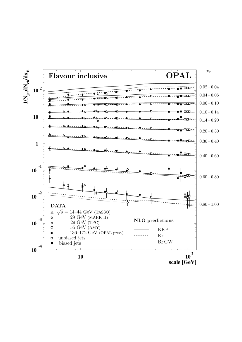
Figure 10: Scale dependence of the flavour inclusive fragmentation functions in different $x_{\mathrm{E}}$ bins. The scale denotes $Q_{\mathrm{j}et}$ for the biased jets and $\sqrt{s}/2$ for the unbiased jets. The inner error bars indicate the statistical uncertainties, the total error bars show the statistical and systematic uncertainties added in quadrature. The values are given in Table 6. In addition, the published unbiased jet data by TASSO, TPC, MARK II, AMY [8] and OPAL [32, 33, 34] are shown. The data are compared to the NLO predictions by KKP [17], Kr [18] and BFGW [19].

In Figs. 7–10 and in Tables 3–6 the results for the udsc, b, gluon and flavour inclusive jet fragmentation functions are presented. The LEP1 unbiased jet data correspond to $\sqrt{s}=91.2$ GeV. Concerning the LEP2 unbiased jets, the b jet fragmentation functions are measured in the entire available $\sqrt{s}$ range of 183–209 GeV. The corresponding data points are placed at $\langle\sqrt{s}\rangle=197$ GeV, where $\langle\sqrt{s}\rangle$ is the luminosity weighted value of $\sqrt{s}$. The udsc and flavour inclusive jet fragmentation functions are measured in three $\sqrt{s}$ intervals: 183–189, 192–202 and 204–209 GeV. The corresponding data points are placed at $\langle\sqrt{s}\rangle$ = 187.6, 198.0 and 206.2 GeV, respectively. The quark biased jet data from LEP1 cover the region $Q_{\mathrm{j}et}=$ 4–42 GeV, while those from LEP2 cover the region $Q_{\mathrm{j}et}=$ 30–105 GeV. The results from the region $0.01<x_{\mathrm{E}}<0.03$ are not shown but they are discussed in Section 8.2. The results are found to be consistent with previous measurements. The fragmentation functions from unbiased quark jets agree to within the total uncertainties with previous OPAL unbiased jet measurements of flavour inclusive and b jet fragmentation functions at $\sqrt{s}=$ 91.2 GeV in [10] and flavour inclusive jet fragmentation functions at $\sqrt{s}=$ 192–209 GeV in [35] (not shown). Similarly, the udsc and gluon fragmentation functions from biased jets agree with similar measurements presented by the DELPHI Collaboration [5] for $Q_{\mathrm{j}et}$ scales between 4 and 30 GeV (not shown). Finally, our gluon jet results are seen to be consistent with the results of the ${\mathrm{g}_{incl}}$ jets [4] at 40.1 GeV, see Fig. 9. The other results from our study represent first measurements, specifically the udsc jet results above 45.6 GeV, the gluon jet results above 30 GeV (except for the ${\mathrm{g}_{incl}}$ jets), and the b jet results at all scales except 45.6 GeV.

The data are compared to the theoretical predictions described in Section 7. For the udsc jet fragmentation function (Fig. 7), all three theoretical predictions give a good description in the entire measured phase space, except for the lowest $x_{\mathrm{E}}$ bin where the KKP calculations overestimate the data, and the highest $x_{\mathrm{E}}$ bin where the data are underestimated by the Kr and BFGW calculations.

The situation is rather different for the b and gluon jet fragmentation functions (Figs. 8 and 9) where the description of the data by the NLO predictions is worse and where there are significant differences between individual NLO results. The latter is, nevertheless, expected due to differences in the calculations such as those discussed in Section 7. In Fig. 8 the KKP prediction is deficient with respect to the data for $x_{\mathrm{E}}>0.12$. As shown in [9], with rising particle momentum, this region is increasingly populated by the products of B hadron decays. It is, however, important to note that these B hadron decay products are indirectly included in theory predictions since they are present in the data sets to which the fits were made.

For the gluon jet fragmentation functions, the two alternative methods of identifying gluon jets described in Section 5.2 are examined, see Fig. 9 and Table 5. The $Q_{\mathrm{j}et}$ binning is not the same for the two methods because of their different regions of applicability. In the LEP1 samples, the interval $Q_{\mathrm{j}et}=$ 4–42 GeV is used for the b-tag method, while for the energy-ordering method, the $Q_{\mathrm{j}et}$ spectra of jets 2 and 3 overlap in the interval $Q_{\mathrm{j}et}=$ 6–27 GeV as mentioned in Section 5.2.2. In the LEP2 samples, the results correspond to the interval $Q_{\mathrm{j}et}=$ 30–70 GeV for the b-tag method, where only jets 2 and 3 are used, and to the interval $Q_{\mathrm{j}et}=$ 30–60 GeV for the energy-ordering method. A satisfactory correspondence between the b-tag and energy-ordering methods is found in the entire scale range accessible. The data tend to show larger scaling violations than predicted by any of the calculations.

The results for the flavour inclusive jet fragmentation functions are presented in Fig. 10 and in Table 6. The results are compared with published unbiased jet data from lower energy e⁺e^- experiments (TASSO, MARK II, TPC and AMY) [8] and previous OPAL results [32, 33, 34]. We note that the fragmentation functions measured by TASSO, MARK II and AMY are defined via $x_{\mathrm{p}}=2p/\sqrt{s}$, where $p$ is particle momentum, rather than via $x_{\mathrm{E}}$ used in the present analysis. This difference in definition leads to non-negligible differences in the region of $x_{\mathrm{E}}<0.1$ and $\sqrt{s}<22$ GeV, therefore the published data from this region are not shown in Fig. 10. The results from the current study are seen to be consistent with the previous results. The data are also compared to the NLO predictions of KKP, Kr and BFGW. All three predictions give a reasonable description of the data in the central region of $x_{\mathrm{E}}$ ($0.06\lesssim x_{\mathrm{E}}\lesssim 0.60$) and over the entire scale range.

A good correspondence is found between the results from biased and unbiased jets in all four figures. This observation suggests that $Q_{\mathrm{j}et}$ is an appropriate choice of scale in three-jet events with a general topology. A similar conclusion was previously presented in [5]. The Monte Carlo study described in Section 6, however, demonstrates that the bias introduced by using jet algorithms in the gluon jet identification is not negligible for $x_{\mathrm{E}}>0.6$. In each of these figures, the scaling violation seen in the data is positive for low $x_{\mathrm{E}}$ and negative for high $x_{\mathrm{E}}$. It is more pronounced in the gluon jets than in the quark jets.

8.2 $\boldmath x_{\boldmath\mathrm{E}}$-dependence

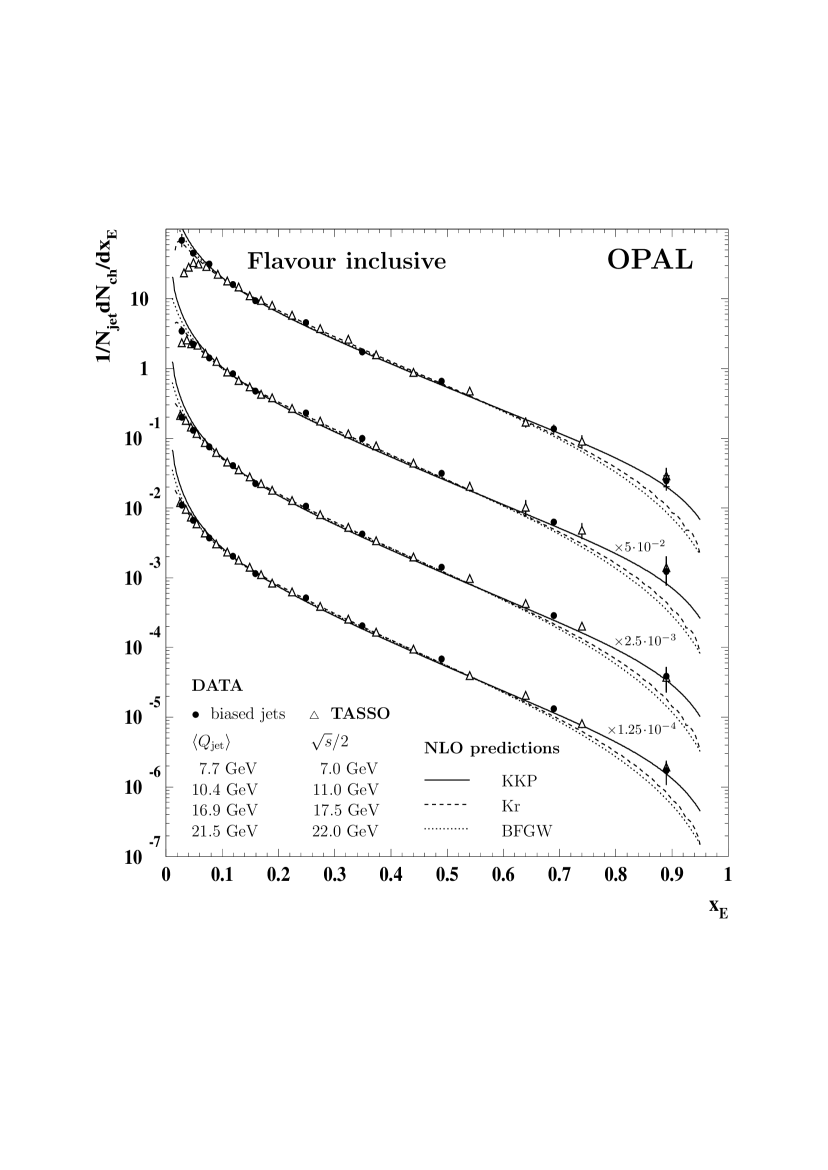
Figure 11: $x_{\mathrm{E}}$ dependence of the flavour inclusive fragmentation functions at different scales. The inner error bars indicate the statistical uncertainties, the total error bars show the statistical and systematic uncertainties added in quadrature. The values are given in Table 6. The results from the biased jets are compared to the results from the unbiased jets of TASSO [8]. The data are compared to the NLO predictions by KKP [17], Kr [18] and BFGW [19]. The results are scaled as indicated in figure.

In Section 6, we noted the region of small $x_{\mathrm{E}}$ with small scales where large differences between biased and unbiased jet fragmentation functions constructed from hadron level MC were observed. In Fig. 11, this observation is confronted with data. We plot again the unbiased jet data of TASSO and the biased jet data from our analysis (Table 6), the latter in those $Q_{\mathrm{j}et}$ bins which correspond well to the c.m.s. energies used in TASSO measurement. We transforme $x_{\mathrm{p}}\rightarrow x_{\mathrm{E}}$ using the pion mass and shifte the TASSO points accordingly. In the first scale bin, the unbiased jet fragmentation functions exhibit turn-over points at very low $x_{\mathrm{E}}$, while the biased jet data grow steeply with decreasing $x_{\mathrm{E}}$. This difference qualitatively confirms the observation we made in point a) of Section 6 using MC jet samples. Further, as anticipated in Section 6, the biased jet data agree better with theory than the unbiased jet data.

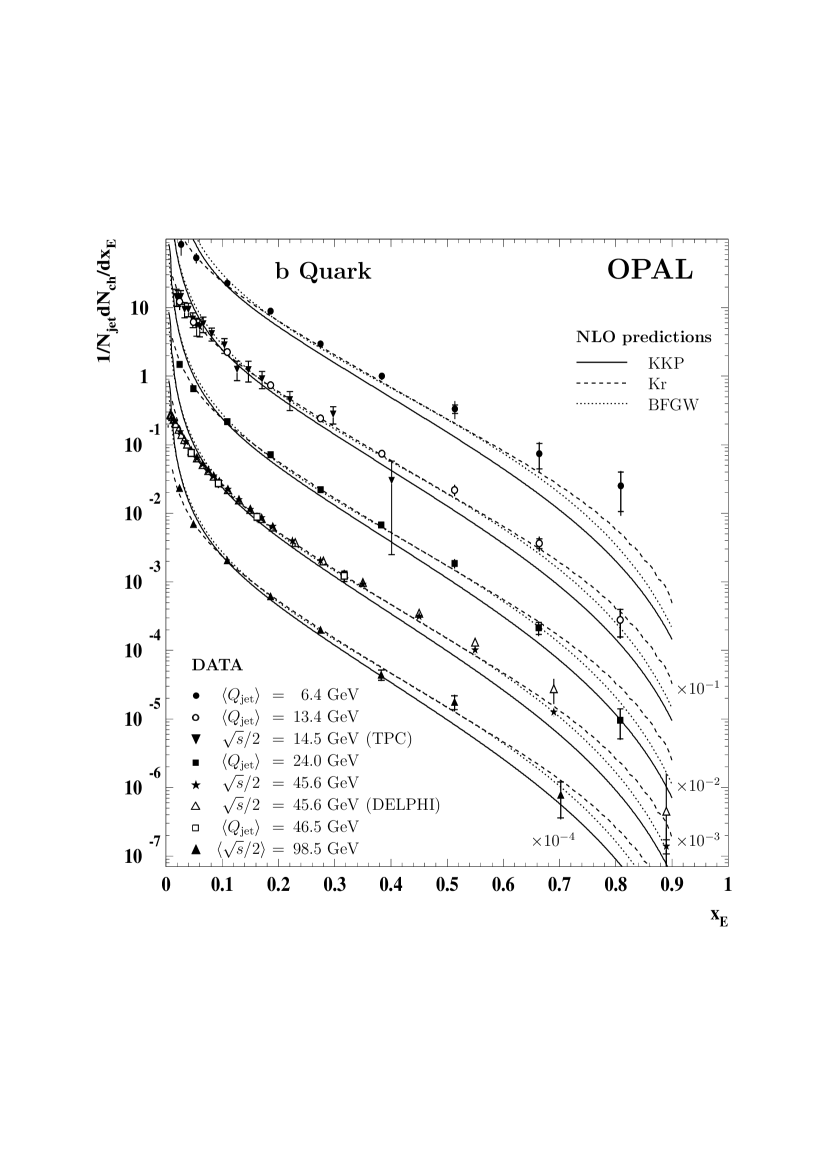
Figure 13: $x_{\mathrm{E}}$ dependence of the b jet fragmentation functions at different scales. The inner error bars indicate the statistical uncertainties, the total error bars show the statistical and systematic uncertainties added in quadrature. The values are given in Table 7. For comparison, the published results on the unbiased jets of DELPHI [9] and the results based on TPC data [8] are shown. The data are compared to the NLO predictions by KKP [17], Kr [18] and BFGW [19]. The results are scaled as indicated in figure.

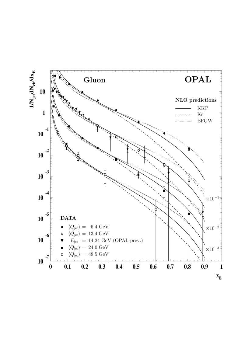
Figure 14: $x_{\mathrm{E}}$ dependence of the gluon jet fragmentation functions at different scales. The inner error bars indicate the statistical uncertainties, the total error bars show the statistical and systematic uncertainties added in quadrature. The values are given in Table 7. Also shown are the recent OPAL results on the boosted gluon jets [14]. The data are compared to the NLO predictions by KKP [17], Kr [18] and BFGW [19]. The results are scaled as indicated in figure.

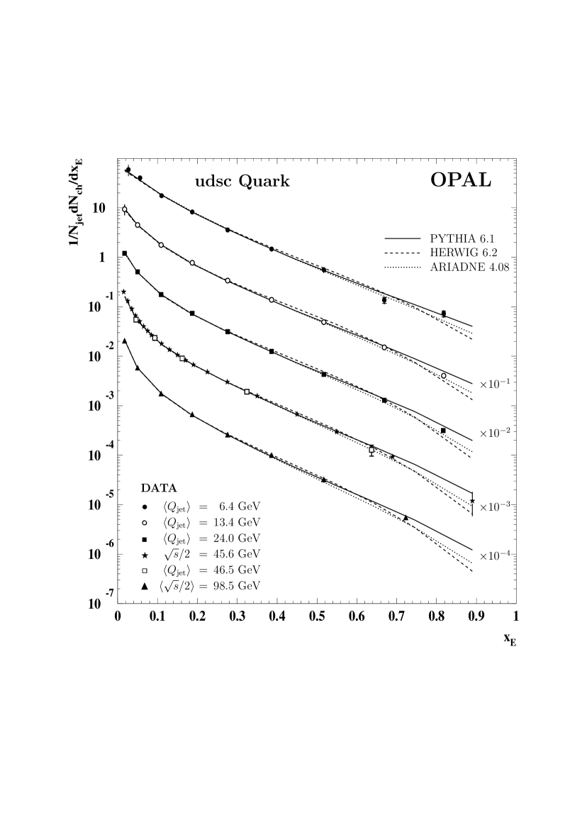
Figure 15: $x_{\mathrm{E}}$ dependence of the udsc jet fragmentation functions at different scales compared with the PYTHIA 6.125, HERWIG 6.2 and ARIADNE 4.08 Monte Carlo predictions. The inner error bars indicate the statistical uncertainties, the total error bars show the statistical and systematic uncertainties added in quadrature. The values are given in Table 7. The results are scaled as indicated in figure.

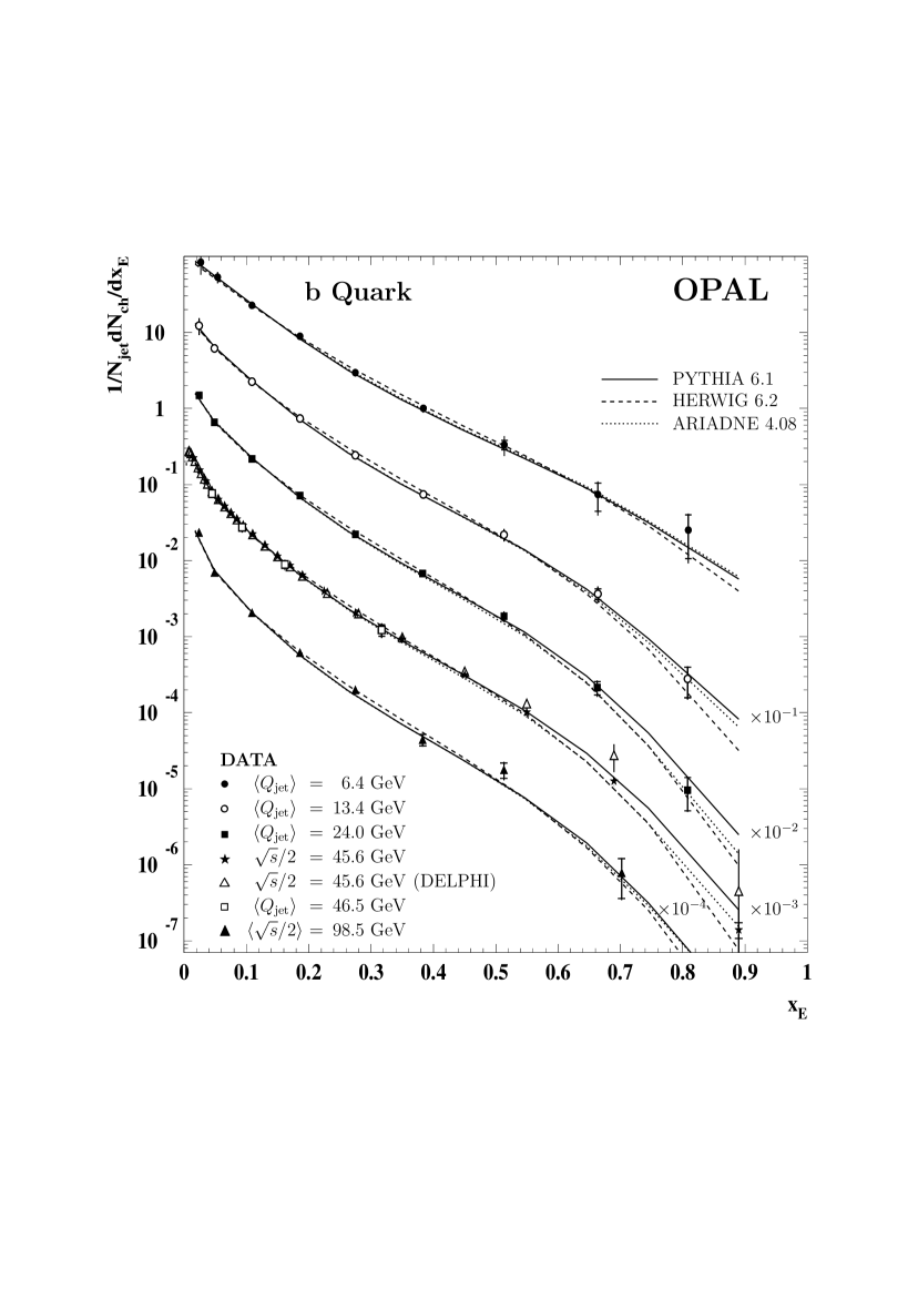
Figure 16: $x_{\mathrm{E}}$ dependence of the b jet fragmentation functions at different scales compared with the PYTHIA 6.125, HERWIG 6.2 and ARIADNE 4.08 Monte Carlo predictions. The inner error bars indicate the statistical uncertainties, the total error bars show the statistical and systematic uncertainties added in quadrature. The values are given in Table 7. For comparison, the published results on the unbiased jets of DELPHI [9] are shown. The results are scaled as indicated in figure.

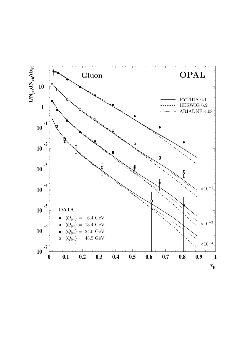
Figure 17: $x_{\mathrm{E}}$ dependence of the gluon jet fragmentation functions at different scales compared with the PYTHIA 6.125, HERWIG 6.2 and ARIADNE 4.08 Monte Carlo predictions. The inner error bars indicate the statistical uncertainties, the total error bars show the statistical and systematic uncertainties added in quadrature. The values are given in Table 7. The results are scaled as indicated in figure.

In Figs. 12–17 we present the results shown in Figs. 7–9 but now in a finer $x_{\mathrm{E}}$ binning and with the additional data from the region $0.01<x_{\mathrm{E}}<0.03$, see Table 7. We integrate over the fragmentation functions in four or five scale intervals: $Q_{\mathrm{j}et}=$ 4–9, 9–19, 19–30, 30–70 and $\sqrt{s}/2=$ 91.5–104.5 GeV. Reference values for these intervals, evaluated as explained at the beginning of this section, are 6.4, 13.4, 24.0, 46.5 (48.5 for gluons) and 98.5 GeV, respectively. In the lowest scale interval, the data in the region of $0.01<x_{\mathrm{E}}<0.02$ are not measured due to the large dependence on the jet algorithm.

In Figs. 12–14 the data are compared to the NLO predictions. In general, the theory predictions are in a good agreement with the measurements of the udsc jet fragmentation function (Fig. 12). We observe that the data in the region of low $x_{\mathrm{E}}$ are overestimated by the predictions of KKP, while they are in agreement with those of Kr and BFGW. For high $x_{\mathrm{E}}$, the data prefer the KKP predictions but the differences between the predictions decrease with increasing scale. In Fig. 13 the measured b jet fragmentation function is shown together with the published results from DELPHI [9] and TPC [48]. Analogously to Fig. 8, the spread of the NLO predictions is larger than that for the udsc jet fragmentation functions. The NLO predictions by Kr are seen to provide a reasonable description of all the b-jet data, while those by KKP and BFGW generally overestimate the data in the region of low $x_{\mathrm{E}}$ and underestimate them for large $x_{\mathrm{E}}$. A possible explanation for this difference is that, unlike KKP or BFGW, the fitting procedure of Kr includes both the low $x_{\mathrm{E}}$ (down to $x_{\mathrm{E}}=0.05$) and low scale data (TPC data [48] taken at $\sqrt{s}=$29 GeV). In Fig. 14 the measured gluon jet fragmentation functions are shown along with the OPAL [14] measurement at $E_{\mathrm{j}et}=$ 14.24 GeV. An overall agreement is found between the results of the boost method and the method used here. The observed sizable spread of the NLO predictions is expected because of the different approaches to the fitting procedures of the gluon jet data (see Section 7).

To test various fragmentation models, the data are also compared in Figs. 15–17 to the hadron level predictions of the PYTHIA 6.125, HERWIG 6.2 and ARIADNE 4.08 MC event generators. The hadron level is defined in Section 5.4. Globally, all MC models give a more satisfactory description of the data than do the NLO predictions. This is presumably due to the fact that the biased jet data are compared to the biased jet MC predictions and the unbiased jet data to the unbiased jet MC predictions. We note that although all MC models used in this study were previously tuned to LEP1 data, they still provide a good description of the LEP2 data. There exist some discrepancies in the description of the gluon jet data in the region of high $x_{\mathrm{E}}$ with small scales (Fig. 17). A good agreement is achieved for the b jet fragmentation functions by all three models.

8.3 Charged particle multiplicities

By integrating the unbiased jet fragmentation functions, the charged particle multiplicities in udsc, b and inclusive hadronic events can be obtained. The results for the LEP2 data are presented in the $\sqrt{s}$ intervals specified above, namely 183–189, 192–202 and 204–209 GeV for the inclusive hadronic and udsc events and 183–209 GeV for the b events.

$\ \ \ \ \ \langle\sqrt{s}\rangle$	$\ \ \ \ \ \ \ \langle n_{\mathrm{c}h}^{\mathrm{i}ncl}\rangle$	$\ \ \ \ \ \ \ \langle n_{\mathrm{c}h}^{\mathrm{u}dsc}\rangle$	$\ \ \ \ \ \ \ \langle n_{\mathrm{c}h}^{\mathrm{b}}\rangle$
$\ \,91.2$ GeV:	$20.93\pm 0.01\pm 0.23$	$20.32\pm 0.03\pm 0.27$	$23.28\pm 0.09\pm 0.70$
187.6 GeV:	$26.80\pm 0.24\pm 0.46$	$26.43\pm 0.26\pm 0.81$
197.0 GeV:			$30.01\pm 0.53\pm 0.82$
198.0 GeV:	$27.68\pm 0.26\pm 0.50$	$27.38\pm 0.31\pm 0.85$
206.2 GeV:	$27.75\pm 0.29\pm 0.67$	$26.87\pm 0.32\pm 0.99$

The results are found to be in agreement with the previous unbiased jet measurements [10, 9, 53]. We also observed a good agreement between the data and predictions of the three MC models used in this analysis. The results for $\langle n_{\mathrm{c}h}^{\mathrm{u}dsc}\rangle$ above 91.2 GeV energy represent new measurements.

9 Conclusions

Scaling violations of quark and gluon jet fragmentation functions are studied in e⁺e^- annihilations at $\sqrt{s}=$ 91.2 and 183–209 GeV using data collected with the OPAL detector at LEP. The scale dependence of the flavour inclusive, udsc and b fragmentation functions from unbiased jets is measured at $\sqrt{s}/2=$ 45.6 and 91.5–104.5 GeV. Biased jets are used to extract the flavour inclusive, udsc and b, and gluon fragmentation functions in the ranges $Q_{\mathrm{j}et}=$ 4–42, 4–105 and 4–70 GeV, respectively, where $Q_{\mathrm{j}et}$ is the jet energy scale. Three methods are used to extract the fragmentation functions, namely the b-tag and energy-ordering methods for biased jets, and the hemisphere method for unbiased jets. The results obtained using these methods are found to be consistent with each other. The udsc jet results above the scale of 45.6 GeV, the gluon jet results above 30 GeV (except for the scale of 40.1 GeV), and the b jet results at all scales except 45.6 GeV represent new measurements. The results of this analysis are compared with existing lower energy e⁺e^- data and with previous results from DELPHI and OPAL. The overall consistency of the biased jet results with the unbiased jet results suggests that $Q_{\mathrm{j}et}$ is a generally appropriate scale in events with a general three-jet topology. The scaling violation is observed to be positive for lower $x_{\mathrm{E}}$ and negative for higher $x_{\mathrm{E}}$, for all the types of fragmentation functions. The gluon jet fragmentation function exhibits stronger scaling violation than that of udsc jets.

The bias of the procedure used to construct biased jet fragmentation functions is estimated by studying hadron level Monte Carlo generator events. In explaining the observed differences between biased and unbiased jet results, we note the effects of non-negligible masses of hadrons and b-quarks at low scales. Due to the considerable bias found for the gluon jet fragmentation functions in the region of $x_{\mathrm{E}}>0.6$, precautions should be taken when comparing the biased gluon jet results with theory.

The data are compared to the predictions of NLO calculations. In a wide range of $x_{\mathrm{E}}$, all calculations satisfactorily describe the data for the udsc jet fragmentation functions. The description is worse and the spread between the predictions larger for the b and gluon jet fragmentation functions, in particular in regions of very low and high $x_{\mathrm{E}}$.

The data are also compared with predictions of three Monte Carlo models, PYTHIA 6.125, HERWIG 6.2 and ARIADNE 4.08. A reasonable agreement with data is observed for all models, except for high $x_{\mathrm{E}}$ region with small scales ($\lesssim$ 14 GeV) in case of the udsc and gluon jet fragmentation functions.

The charged particle multiplicities of udsc, b and inclusive hadronic events are obtained by integrating the measured fragmentation functions. All values are found to be in agreement with previous measurements, where available.

Selection	Data LEP1	Data LEP2	BG(LEP2)
Hadronic events	2 387 227	10 866 (12 653)	11% (14%)
three-jet events	965 513	6 177	16%
udsc jets	2 675 679	16 344	16%
b-tag jets	83 549	820	9%
Gluon jets	73 620	729	9%
udsc hemispheres	4 740 774	20 146	11%
b-tag hemispheres	33 680	1 586	5%

Table 1: Statistics of the LEP1 and LEP2 data samples. The number of hadronic events is given (the numbers in brackets correspond to LEP2 events used for three-jet analysis) and the characteristics of the biased jet samples (number of three-jet events, udsc, b-tag and gluon jets) and the unbiased jet samples (number of udsc and b-tag hemispheres) are shown. The jets are found by the Durham jet algorithm. Also indicated is the percentage of the remaining 4-fermion background (BG) for the LEP2 data. For the LEP1 data, the background is negligible.

Cuts	Loss [%]
	LEP1	LEP2
Particle multiplicity per jet $\geq$ 2	0.7	1.7
Sum of inter-jet angles $\geq 358^{\circ}$	3.9	2.3
Polar jet angle $|\cos\theta_{\rm jet}|\leq 0.90\ (0.95)$	8.4	2.3
Corrected jet energy $\geq$ 5 GeV	11.2	5.9
Inter-jet angle $\geq 30^{\circ}$	43.3	43.2

Table 2: Jet selection cuts for the LEP1 and LEP2 data and the reduction of statistics found by imposing each cut individually after the hadronic event selection. The jets are found by the Durham jet algorithm. The cut value given in brackets corresponds to the LEP2 selection.

$x_{\mathrm{E}}$	scale [GeV]		$\frac{1}{N_{\mathrm{j}et}^{\mathrm{u}dsc}}\frac{{\mathrm{d}}N_{\mathrm{c}h}}{{\mathrm{d}}x_{\mathrm{E}}}$			$x_{\mathrm{E}}$	scale [GeV]		$\frac{1}{N_{\mathrm{j}et}^{\mathrm{u}dsc}}\frac{{\mathrm{d}}N_{\mathrm{c}h}}{{\mathrm{d}}x_{\mathrm{E}}}$
0.03–0.07	4.0  –	6.5	38.1	$\!\!\!\!\pm$1.5	$\!\!\!\!\pm$4.0	0.22–0.48	4.0  –	6.5	2.54	$\!\!\!\!\pm$0.14	$\!\!\!\!\pm$0.17
	6.5  –	9.0	45.5	$\!\!\!\!\pm$1.1	$\!\!\!\!\pm$4.7		6.5  –	9.0	2.28	$\!\!\!\!\pm$0.07	$\!\!\!\!\pm$0.15
	9.0  –	12.0	44.8	$\!\!\!\!\pm$0.7	$\!\!\!\!\pm$2.3		9.0  –	12.0	2.383	$\!\!\!\!\pm$0.037	$\!\!\!\!\pm$0.063
	12.0  –	15.0	49.8	$\!\!\!\!\pm$0.7	$\!\!\!\!\pm$2.6		12.0  –	15.0	2.205	$\!\!\!\!\pm$0.032	$\!\!\!\!\pm$0.059
	15.0  –	19.0	51.9	$\!\!\!\!\pm$0.6	$\!\!\!\!\pm$2.7		15.0  –	19.0	2.142	$\!\!\!\!\pm$0.027	$\!\!\!\!\pm$0.057
	19.0  –	24.0	54.12	$\!\!\!\!\pm$0.55	$\!\!\!\!\pm$0.94		19.0  –	24.0	2.074	$\!\!\!\!\pm$0.024	$\!\!\!\!\pm$0.026
	24.0  –	30.0	57.31	$\!\!\!\!\pm$0.51	$\!\!\!\!\pm$0.99		24.0  –	30.0	2.017	$\!\!\!\!\pm$0.022	$\!\!\!\!\pm$0.025
	30.0  –	42.0	55.6	$\!\!\!\!\pm$0.2	$\!\!\!\!\pm$2.2		30.0  –	42.0	2.058	$\!\!\!\!\pm$0.011	$\!\!\!\!\pm$0.099
	30.0  –	47.0	49.3	$\!\!\!\!\pm$4.9	$\!\!\!\!\pm$3.8		30.0  –	47.0	2.05	$\!\!\!\!\pm$0.21	$\!\!\!\!\pm$0.17
	45.6		61.80	$\!\!\!\!\pm$0.08	$\!\!\!\!\pm$0.82		45.6		1.899	$\!\!\!\!\pm$0.004	$\!\!\!\!\pm$0.038
	47.0  –	70.0	60.6	$\!\!\!\!\pm$3.2	$\!\!\!\!\pm$4.7		47.0  –	70.0	1.68	$\!\!\!\!\pm$0.25	$\!\!\!\!\pm$0.14
	70.0  –	105.0	61.1	$\!\!\!\!\pm$5.6	$\!\!\!\!\pm$9.5		70.0  –	105.0	1.93	$\!\!\!\!\pm$0.28	$\!\!\!\!\pm$0.33
	93.8		64.1	$\!\!\!\!\pm$0.8	$\!\!\!\!\pm$2.1		93.8		1.724	$\!\!\!\!\pm$0.040	$\!\!\!\!\pm$0.040
	99.0		65.3	$\!\!\!\!\pm$0.9	$\!\!\!\!\pm$2.6		99.0		1.629	$\!\!\!\!\pm$0.047	$\!\!\!\!\pm$0.042
	103.1		64.3	$\!\!\!\!\pm$1.0	$\!\!\!\!\pm$2.1		103.1		1.695	$\!\!\!\!\pm$0.050	$\!\!\!\!\pm$0.037
0.07–0.12	4.0  –	6.5	20.9	$\!\!\!\!\pm$1.0	$\!\!\!\!\pm$1.0	0.48–0.90	4.0  –	6.5	0.214	$\!\!\!\!\pm$0.031	$\!\!\!\!\pm$0.026
	6.5  –	9.0	23.9	$\!\!\!\!\pm$0.6	$\!\!\!\!\pm$1.1		6.5  –	9.0	0.219	$\!\!\!\!\pm$0.013	$\!\!\!\!\pm$0.026
	9.0  –	12.0	22.46	$\!\!\!\!\pm$0.37	$\!\!\!\!\pm$0.57		9.0  –	12.0	0.201	$\!\!\!\!\pm$0.006	$\!\!\!\!\pm$0.012
	12.0  –	15.0	22.55	$\!\!\!\!\pm$0.35	$\!\!\!\!\pm$0.57		12.0  –	15.0	0.183	$\!\!\!\!\pm$0.006	$\!\!\!\!\pm$0.011
	15.0  –	19.0	22.88	$\!\!\!\!\pm$0.31	$\!\!\!\!\pm$0.58		15.0  –	19.0	0.180	$\!\!\!\!\pm$0.005	$\!\!\!\!\pm$0.011
	19.0  –	24.0	23.16	$\!\!\!\!\pm$0.27	$\!\!\!\!\pm$0.74		19.0  –	24.0	0.1697	$\!\!\!\!\pm$0.0040	$\!\!\!\!\pm$0.0076
	24.0  –	30.0	22.61	$\!\!\!\!\pm$0.26	$\!\!\!\!\pm$0.72		24.0  –	30.0	0.1581	$\!\!\!\!\pm$0.0036	$\!\!\!\!\pm$0.0071
	30.0  –	42.0	22.60	$\!\!\!\!\pm$0.12	$\!\!\!\!\pm$0.91		30.0  –	42.0	0.1633	$\!\!\!\!\pm$0.0015	$\!\!\!\!\pm$0.0043
	30.0  –	47.0	23.4	$\!\!\!\!\pm$2.2	$\!\!\!\!\pm$1.4		–			–
	45.6		23.57	$\!\!\!\!\pm$0.04	$\!\!\!\!\pm$0.24		45.6		0.1411	$\!\!\!\!\pm$0.0005	$\!\!\!\!\pm$0.0058
	47.0  –	70.0	23.3	$\!\!\!\!\pm$2.0	$\!\!\!\!\pm$1.4		30.0  –	70.0	0.128	$\!\!\!\!\pm$0.032	$\!\!\!\!\pm$0.013
	70.0  –	105.0	21.3	$\!\!\!\!\pm$2.7	$\!\!\!\!\pm$3.3		70.0  –	105.0	0.052	$\!\!\!\!\pm$0.073	$\!\!\!\!\pm$0.019
	93.8		23.10	$\!\!\!\!\pm$0.41	$\!\!\!\!\pm$0.64		93.8		0.1231	$\!\!\!\!\pm$0.0079	$\!\!\!\!\pm$0.0060
	99.0		23.89	$\!\!\!\!\pm$0.46	$\!\!\!\!\pm$0.99		99.0		0.1154	$\!\!\!\!\pm$0.0091	$\!\!\!\!\pm$0.0060
	103.1		23.37	$\!\!\!\!\pm$0.52	$\!\!\!\!\pm$0.75		103.1		0.1289	$\!\!\!\!\pm$0.0095	$\!\!\!\!\pm$0.0062
0.12–0.22	4.0  –	6.5	10.25	$\!\!\!\!\pm$0.47	$\!\!\!\!\pm$0.69
	6.5  –	9.0	9.81	$\!\!\!\!\pm$0.26	$\!\!\!\!\pm$0.66
	9.0  –	12.0	9.81	$\!\!\!\!\pm$0.15	$\!\!\!\!\pm$0.35
	12.0  –	15.0	9.87	$\!\!\!\!\pm$0.14	$\!\!\!\!\pm$0.35
	15.0  –	19.0	9.44	$\!\!\!\!\pm$0.12	$\!\!\!\!\pm$0.34
	19.0  –	24.0	9.38	$\!\!\!\!\pm$0.10	$\!\!\!\!\pm$0.14
	24.0  –	30.0	9.36	$\!\!\!\!\pm$0.09	$\!\!\!\!\pm$0.14
	30.0  –	42.0	9.23	$\!\!\!\!\pm$0.05	$\!\!\!\!\pm$0.25
	30.0  –	47.0	9.60	$\!\!\!\!\pm$0.81	$\!\!\!\!\pm$0.58
	45.6		8.98	$\!\!\!\!\pm$0.02	$\!\!\!\!\pm$0.14
	47.0  –	70.0	8.24	$\!\!\!\!\pm$0.89	$\!\!\!\!\pm$0.49
	70.0  –	105.0	7.7	$\!\!\!\!\pm$1.1	$\!\!\!\!\pm$0.8
	93.8		8.92	$\!\!\!\!\pm$0.17	$\!\!\!\!\pm$0.16
	99.0		8.48	$\!\!\!\!\pm$0.19	$\!\!\!\!\pm$0.29
	103.1		8.68	$\!\!\!\!\pm$0.20	$\!\!\!\!\pm$0.08

Table 3: The udsc jet fragmentation function in bins of $x_{\mathrm{E}}$ and scale. The scale denotes $Q_{\mathrm{j}et}$ for the biased jets and is given by the intervals, while it denotes $\sqrt{s}/2$ for the unbiased jets and is given by the single values. The first uncertainty is statistical, the second systematic. These data are displayed in Fig. 7.

$x_{\mathrm{E}}$	scale [GeV]		$\frac{1}{N_{\mathrm{j}et}^{\mathrm{b}}}\frac{{\mathrm{d}}N_{\mathrm{c}h}}{{\mathrm{d}}x_{\mathrm{E}}}$			$x_{\mathrm{E}}$	scale [GeV]		$\frac{1}{N_{\mathrm{j}et}^{\mathrm{b}}}\frac{{\mathrm{d}}N_{\mathrm{c}h}}{{\mathrm{d}}x_{\mathrm{E}}}$
0.03–0.07	4.0  –	6.5	51.2	$\!\!\!\!\pm$2.1	$\!\!\!\!\pm$8.9	0.22–0.48	4.0  –	6.5	2.10	$\!\!\!\!\pm$0.15	$\!\!\!\!\pm$0.20
	6.5  –	9.0	61	$\!\!\!\!\pm$1	$\!\!\!\!\pm$11		6.5  –	9.0	1.74	$\!\!\!\!\pm$0.06	$\!\!\!\!\pm$0.16
	9.0  –	12.0	65.6	$\!\!\!\!\pm$0.8	$\!\!\!\!\pm$4.5		9.0  –	12.0	1.53	$\!\!\!\!\pm$0.04	$\!\!\!\!\pm$0.13
	12.0  –	15.0	65.7	$\!\!\!\!\pm$0.7	$\!\!\!\!\pm$4.5		12.0  –	15.0	1.45	$\!\!\!\!\pm$0.04	$\!\!\!\!\pm$0.12
	15.0  –	19.0	69.9	$\!\!\!\!\pm$0.7	$\!\!\!\!\pm$4.8		15.0  –	19.0	1.43	$\!\!\!\!\pm$0.03	$\!\!\!\!\pm$0.12
	19.0  –	24.0	70.8	$\!\!\!\!\pm$0.6	$\!\!\!\!\pm$2.9		19.0  –	24.0	1.360	$\!\!\!\!\pm$0.029	$\!\!\!\!\pm$0.055
	24.0  –	30.0	72.2	$\!\!\!\!\pm$0.6	$\!\!\!\!\pm$3.0		24.0  –	30.0	1.359	$\!\!\!\!\pm$0.026	$\!\!\!\!\pm$0.055
	30.0  –	42.0	71.4	$\!\!\!\!\pm$0.3	$\!\!\!\!\pm$3.3		30.0  –	42.0	1.373	$\!\!\!\!\pm$0.015	$\!\!\!\!\pm$0.022
	30.0  –	47.0	72.9	$\!\!\!\!\pm$6.4	$\!\!\!\!\pm$5.1		30.0  –	47.0	1.37	$\!\!\!\!\pm$0.31	$\!\!\!\!\pm$0.19
	45.6		76.9	$\!\!\!\!\pm$0.2	$\!\!\!\!\pm$1.9		45.6		1.253	$\!\!\!\!\pm$0.011	$\!\!\!\!\pm$0.064
	47.0  –	70.0	77.0	$\!\!\!\!\pm$6.2	$\!\!\!\!\pm$5.4		47.0  –	70.0	1.12	$\!\!\!\!\pm$0.29	$\!\!\!\!\pm$0.15
	70.0  –	105.0	74.3	$\!\!\!\!\pm$4.8	$\!\!\!\!\pm$7.3		70.0  –	105.0	1.34	$\!\!\!\!\pm$0.21	$\!\!\!\!\pm$0.18
	98.5		77.4	$\!\!\!\!\pm$1.7	$\!\!\!\!\pm$1.7		98.5		1.112	$\!\!\!\!\pm$0.075	$\!\!\!\!\pm$0.089
0.07–0.12	4.0  –	6.5	28.7	$\!\!\!\!\pm$1.3	$\!\!\!\!\pm$1.5	0.48–0.90	4.0  –	6.5	0.134	$\!\!\!\!\pm$0.046	$\!\!\!\!\pm$0.034
	6.5  –	9.0	30.1	$\!\!\!\!\pm$0.7	$\!\!\!\!\pm$1.6		6.5  –	9.0	0.111	$\!\!\!\!\pm$0.020	$\!\!\!\!\pm$0.028
	9.0  –	12.0	30.32	$\!\!\!\!\pm$0.42	$\!\!\!\!\pm$0.48		9.0  –	12.0	0.076	$\!\!\!\!\pm$0.010	$\!\!\!\!\pm$0.013
	12.0  –	15.0	30.77	$\!\!\!\!\pm$0.41	$\!\!\!\!\pm$0.49		12.0  –	15.0	0.066	$\!\!\!\!\pm$0.008	$\!\!\!\!\pm$0.012
	15.0  –	19.0	30.21	$\!\!\!\!\pm$0.35	$\!\!\!\!\pm$0.48		15.0  –	19.0	0.0564	$\!\!\!\!\pm$0.0067	$\!\!\!\!\pm$0.0099
	19.0  –	24.0	29.96	$\!\!\!\!\pm$0.32	$\!\!\!\!\pm$0.63		19.0  –	24.0	0.0466	$\!\!\!\!\pm$0.0053	$\!\!\!\!\pm$0.0066
	24.0  –	30.0	29.90	$\!\!\!\!\pm$0.29	$\!\!\!\!\pm$0.62		24.0  –	30.0	0.0524	$\!\!\!\!\pm$0.0052	$\!\!\!\!\pm$0.0074
	30.0  –	42.0	29.71	$\!\!\!\!\pm$0.17	$\!\!\!\!\pm$0.60		30.0  –	42.0	0.0476	$\!\!\!\!\pm$0.0029	$\!\!\!\!\pm$0.0068
	30.0  –	47.0	28.6	$\!\!\!\!\pm$3.4	$\!\!\!\!\pm$3.5		30.0  –	47.0		–
	45.6		30.15	$\!\!\!\!\pm$0.12	$\!\!\!\!\pm$0.44		45.6		0.0379	$\!\!\!\!\pm$0.0016	$\!\!\!\!\pm$0.0041
	47.0  –	70.0	26.5	$\!\!\!\!\pm$3.1	$\!\!\!\!\pm$3.3		47.0  –	70.0		–
	70.0  –	105.0	30.9	$\!\!\!\!\pm$2.5	$\!\!\!\!\pm$3.9		70.0  –	105.0	0.056	$\!\!\!\!\pm$0.040	$\!\!\!\!\pm$0.016
	98.5		28.9	$\!\!\!\!\pm$0.9	$\!\!\!\!\pm$1.4		98.5		0.046	$\!\!\!\!\pm$0.011	$\!\!\!\!\pm$0.007
0.12–0.22	4.0  –	6.5	11.80	$\!\!\!\!\pm$0.54	$\!\!\!\!\pm$0.75
	6.5  –	9.0	11.14	$\!\!\!\!\pm$0.25	$\!\!\!\!\pm$0.71
	9.0  –	12.0	10.41	$\!\!\!\!\pm$0.15	$\!\!\!\!\pm$0.47
	12.0  –	15.0	9.94	$\!\!\!\!\pm$0.15	$\!\!\!\!\pm$0.45
	15.0  –	19.0	9.99	$\!\!\!\!\pm$0.13	$\!\!\!\!\pm$0.45
	19.0  –	24.0	9.98	$\!\!\!\!\pm$0.12	$\!\!\!\!\pm$0.28
	24.0  –	30.0	9.58	$\!\!\!\!\pm$0.11	$\!\!\!\!\pm$0.26
	30.0  –	42.0	9.83	$\!\!\!\!\pm$0.06	$\!\!\!\!\pm$0.27
	30.0  –	47.0	8.7	$\!\!\!\!\pm$1.2	$\!\!\!\!\pm$1.2
	45.6		9.40	$\!\!\!\!\pm$0.05	$\!\!\!\!\pm$0.28
	47.0  –	70.0	9.0	$\!\!\!\!\pm$1.1	$\!\!\!\!\pm$1.2
	70.0  –	105.0	8.8	$\!\!\!\!\pm$0.9	$\!\!\!\!\pm$1.0
	98.5		8.94	$\!\!\!\!\pm$0.33	$\!\!\!\!\pm$0.24

Table 4: The b jet fragmentation function in bins of $x_{\mathrm{E}}$ and scale. The scale denotes $Q_{\mathrm{j}et}$ for the biased jets and is given by the intervals, while it denotes $\sqrt{s}/2$ for the unbiased jets and is given by the single values. The first uncertainty is statistical, the second systematic. These data are displayed in Fig. 8. In the region 0.48 $<x_{\mathrm{E}}<$ 0.90 and $Q_{\mathrm{j}et}=$ 30–70 GeV, no measurement was possible due to low statistics.

$x_{\mathrm{E}}$	$Q_{\mathrm{j}et}$ [GeV]		$\frac{1}{N_{\mathrm{j}et}^{\mathrm{g}}}\frac{{\mathrm{d}}N_{\mathrm{c}h}}{{\mathrm{d}}x_{\mathrm{E}}}$ (BT)			$Q_{\mathrm{j}et}$ [GeV]		$\frac{1}{N_{\mathrm{j}et}^{\mathrm{g}}}\frac{{\mathrm{d}}N_{\mathrm{c}h}}{{\mathrm{d}}x_{\mathrm{E}}}$ (EO)
0.03–0.07	4.0  –	6.5	43.3	$\!\!\!\!\pm$0.6	$\!\!\!\!\pm$9.6	6.0   –	6.5	44	$\!\!\!\!\pm$1	$\!\!\!\!\pm$10
	6.5  –	9.0	58.2	$\!\!\!\!\pm$0.6	$\!\!\!\!\pm$9.4	6.5   –	9.0	57.1	$\!\!\!\!\pm$0.4	$\!\!\!\!\pm$6.4
	9.0  –	12.0	69.9	$\!\!\!\!\pm$0.8	$\!\!\!\!\pm$6.4	9.0   –	12.0	68.1	$\!\!\!\!\pm$0.4	$\!\!\!\!\pm$5.8
	12.0  –	15.0	73.8	$\!\!\!\!\pm$1.0	$\!\!\!\!\pm$6.8	12.0   –	15.0	75.7	$\!\!\!\!\pm$0.6	$\!\!\!\!\pm$4.4
	15.0  –	19.0	79.5	$\!\!\!\!\pm$1.3	$\!\!\!\!\pm$7.3	15.0   –	19.0	80.6	$\!\!\!\!\pm$0.8	$\!\!\!\!\pm$4.4
	19.0  –	24.0	84.7	$\!\!\!\!\pm$1.7	$\!\!\!\!\pm$6.8	19.0   –	24.0	85.6	$\!\!\!\!\pm$1.4	$\!\!\!\!\pm$5.2
	24.0  –	30.0	80.5	$\!\!\!\!\pm$2.4	$\!\!\!\!\pm$6.4	24.0   –	27.0	92.4	$\!\!\!\!\pm$5.3	$\!\!\!\!\pm$5.6
	30.0  –	42.0	89	$\!\!\!\!\pm$4	$\!\!\!\!\pm$14	–			–
	30.0  –	70.0	118	$\!\!\!\!\pm$19	$\!\!\!\!\pm$10	30.0   –	60.0	101	$\!\!\!\!\pm$11	$\!\!\!\!\pm$9
0.07–0.12	4.0  –	6.5	26.6	$\!\!\!\!\pm$0.3	$\!\!\!\!\pm$1.4	6.0   –	6.5	27.5	$\!\!\!\!\pm$0.5	$\!\!\!\!\pm$2.3
	6.5  –	9.0	29.7	$\!\!\!\!\pm$0.4	$\!\!\!\!\pm$1.6	6.5   –	9.0	30.4	$\!\!\!\!\pm$0.2	$\!\!\!\!\pm$1.0
	9.0  –	12.0	31.65	$\!\!\!\!\pm$0.43	$\!\!\!\!\pm$0.71	9.0   –	12.0	32.37	$\!\!\!\!\pm$0.21	$\!\!\!\!\pm$0.86
	12.0  –	15.0	32.69	$\!\!\!\!\pm$0.58	$\!\!\!\!\pm$0.74	12.0   –	15.0	33.00	$\!\!\!\!\pm$0.30	$\!\!\!\!\pm$0.81
	15.0  –	19.0	32.14	$\!\!\!\!\pm$0.66	$\!\!\!\!\pm$0.73	15.0   –	19.0	32.90	$\!\!\!\!\pm$0.40	$\!\!\!\!\pm$0.87
	19.0  –	24.0	31.2	$\!\!\!\!\pm$0.9	$\!\!\!\!\pm$1.8	19.0   –	24.0	32.2	$\!\!\!\!\pm$0.7	$\!\!\!\!\pm$1.1
	24.0  –	30.0	33.6	$\!\!\!\!\pm$1.5	$\!\!\!\!\pm$1.9	24.0   –	27.0	34.7	$\!\!\!\!\pm$2.7	$\!\!\!\!\pm$1.2
	30.0  –	42.0	32.7	$\!\!\!\!\pm$2.1	$\!\!\!\!\pm$2.7	–			–
	30.0  –	70.0	27.5	$\!\!\!\!\pm$7.9	$\!\!\!\!\pm$5.2	30.0   –	60.0	30.2	$\!\!\!\!\pm$5.0	$\!\!\!\!\pm$2.8
0.12–0.22	4.0  –	6.5	12.14	$\!\!\!\!\pm$0.15	$\!\!\!\!\pm$0.25	6.0   –	6.5	11.99	$\!\!\!\!\pm$0.19	$\!\!\!\!\pm$0.17
	6.5  –	9.0	11.88	$\!\!\!\!\pm$0.16	$\!\!\!\!\pm$0.24	6.5   –	9.0	12.10	$\!\!\!\!\pm$0.08	$\!\!\!\!\pm$0.21
	9.0  –	12.0	11.12	$\!\!\!\!\pm$0.17	$\!\!\!\!\pm$0.20	9.0   –	12.0	11.49	$\!\!\!\!\pm$0.09	$\!\!\!\!\pm$0.29
	12.0  –	15.0	10.39	$\!\!\!\!\pm$0.22	$\!\!\!\!\pm$0.19	12.0   –	15.0	10.87	$\!\!\!\!\pm$0.12	$\!\!\!\!\pm$0.35
	15.0  –	19.0	10.01	$\!\!\!\!\pm$0.26	$\!\!\!\!\pm$0.18	15.0   –	19.0	10.35	$\!\!\!\!\pm$0.16	$\!\!\!\!\pm$0.26
	19.0  –	24.0	9.26	$\!\!\!\!\pm$0.34	$\!\!\!\!\pm$0.68	19.0   –	24.0	9.54	$\!\!\!\!\pm$0.26	$\!\!\!\!\pm$0.35
	24.0  –	30.0	8.46	$\!\!\!\!\pm$0.52	$\!\!\!\!\pm$0.62	24.0   –	27.0	8.13	$\!\!\!\!\pm$0.86	$\!\!\!\!\pm$0.30
	30.0  –	42.0	7.5	$\!\!\!\!\pm$0.7	$\!\!\!\!\pm$1.7	–			–
	30.0  –	70.0	9.7	$\!\!\!\!\pm$4.1	$\!\!\!\!\pm$2.1	30.0   –	60.0	12.6	$\!\!\!\!\pm$2.2	$\!\!\!\!\pm$2.3
0.22–0.48	4.0  –	6.5	2.603	$\!\!\!\!\pm$0.041	$\!\!\!\!\pm$0.092	6.0   –	6.5	2.59	$\!\!\!\!\pm$0.05	$\!\!\!\!\pm$0.12
	6.5  –	9.0	2.022	$\!\!\!\!\pm$0.038	$\!\!\!\!\pm$0.072	6.5   –	9.0	2.034	$\!\!\!\!\pm$0.020	$\!\!\!\!\pm$0.052
	9.0  –	12.0	1.587	$\!\!\!\!\pm$0.038	$\!\!\!\!\pm$0.076	9.0   –	12.0	1.741	$\!\!\!\!\pm$0.021	$\!\!\!\!\pm$0.071
	12.0  –	15.0	1.527	$\!\!\!\!\pm$0.052	$\!\!\!\!\pm$0.073	12.0   –	15.0	1.589	$\!\!\!\!\pm$0.031	$\!\!\!\!\pm$0.049
	15.0  –	19.0	1.403	$\!\!\!\!\pm$0.062	$\!\!\!\!\pm$0.067	15.0   –	19.0	1.389	$\!\!\!\!\pm$0.039	$\!\!\!\!\pm$0.090
	19.0  –	24.0	1.33	$\!\!\!\!\pm$0.08	$\!\!\!\!\pm$0.13	19.0   –	24.0	1.21	$\!\!\!\!\pm$0.07	$\!\!\!\!\pm$0.18
	24.0  –	30.0	1.35	$\!\!\!\!\pm$0.14	$\!\!\!\!\pm$0.14	24.0   –	27.0	1.14	$\!\!\!\!\pm$0.24	$\!\!\!\!\pm$0.17
	30.0  –	42.0	1.22	$\!\!\!\!\pm$0.18	$\!\!\!\!\pm$0.13	–			–
	30.0  –	70.0	1.21	$\!\!\!\!\pm$0.74	$\!\!\!\!\pm$0.38	30.0   –	60.0	1.03	$\!\!\!\!\pm$0.49	$\!\!\!\!\pm$0.15
0.48–0.90	4.0  –	6.5	0.168	$\!\!\!\!\pm$0.008	$\!\!\!\!\pm$0.026	6.0   –	6.5	0.158	$\!\!\!\!\pm$0.010	$\!\!\!\!\pm$0.023
	6.5  –	9.0	0.085	$\!\!\!\!\pm$0.006	$\!\!\!\!\pm$0.013	6.5   –	9.0	0.099	$\!\!\!\!\pm$0.005	$\!\!\!\!\pm$0.014
	9.0  –	12.0	0.069	$\!\!\!\!\pm$0.007	$\!\!\!\!\pm$0.010	9.0   –	12.0	0.077	$\!\!\!\!\pm$0.006	$\!\!\!\!\pm$0.016
	12.0  –	15.0	0.0527	$\!\!\!\!\pm$0.0072	$\!\!\!\!\pm$0.0078	12.0   –	15.0	0.072	$\!\!\!\!\pm$0.013	$\!\!\!\!\pm$0.023
	15.0  –	19.0	0.0350	$\!\!\!\!\pm$0.0066	$\!\!\!\!\pm$0.0052	15.0   –	19.0	0.047	$\!\!\!\!\pm$0.014	$\!\!\!\!\pm$0.015
	19.0  –	24.0	0.033	$\!\!\!\!\pm$0.009	$\!\!\!\!\pm$0.009	19.0   –	24.0	0.019	$\!\!\!\!\pm$0.047	$\!\!\!\!\pm$0.006
	24.0  –	30.0	0.064	$\!\!\!\!\pm$0.033	$\!\!\!\!\pm$0.017	24.0   –	27.0		–
	30.0  –	42.0		–		–			–
	30.0  –	70.0	0.028	$\!\!\!\!\pm$0.050	$\!\!\!\!\pm$0.017	30.0   –	60.0		–

Table 5: The gluon jet fragmentation functions in bins of $x_{\mathrm{E}}$ and scale $Q_{\mathrm{j}et}$ obtained from the biased jets using the b-tag method (BT) and the energy-ordering method (EO). The first uncertainty is statistical, the second systematic. These data are displayed in Fig. 9. In the region 0.48 $<x_{\mathrm{E}}<$ 0.90 and $Q_{\mathrm{j}et}=$ 30–42 GeV for the b-tag method and $Q_{\mathrm{j}et}=$ 24–60 GeV for the energy-ordering method, no measurement was possible due to low statistics.

$x_{\mathrm{E}}$	scale [GeV]		$\frac{1}{N_{\mathrm{j}et}}\frac{{\mathrm{d}}N_{\mathrm{c}h}}{{\mathrm{d}}x_{\mathrm{E}}}$			$x_{\mathrm{E}}$	scale [GeV]		$\frac{1}{N_{\mathrm{j}et}}\frac{{\mathrm{d}}N_{\mathrm{c}h}}{{\mathrm{d}}x_{\mathrm{E}}}$
0.02–0.04	4.0  –	6.5	46.0	$\!\!\!\!\pm$3.4	$\!\!\!\!\pm$9.3	0.20–0.30	4.0  –	6.5	4.57	$\!\!\!\!\pm$0.46	$\!\!\!\!\pm$0.40
	6.5  –	9.0	69	$\!\!\!\!\pm$2	$\!\!\!\!\pm$14		6.5  –	9.0	4.55	$\!\!\!\!\pm$0.20	$\!\!\!\!\pm$0.40
	9.0  –	12.0	68.9	$\!\!\!\!\pm$1.2	$\!\!\!\!\pm$7.8		9.0  –	12.0	4.58	$\!\!\!\!\pm$0.09	$\!\!\!\!\pm$0.11
	12.0  –	15.0	75.5	$\!\!\!\!\pm$1.2	$\!\!\!\!\pm$8.5		12.0  –	15.0	4.33	$\!\!\!\!\pm$0.08	$\!\!\!\!\pm$0.11
	15.0  –	19.0	80.5	$\!\!\!\!\pm$1.1	$\!\!\!\!\pm$9.1		15.0  –	19.0	4.23	$\!\!\!\!\pm$0.07	$\!\!\!\!\pm$0.10
	19.0  –	24.0	87.7	$\!\!\!\!\pm$1.0	$\!\!\!\!\pm$2.1		19.0  –	24.0	4.098	$\!\!\!\!\pm$0.059	$\!\!\!\!\pm$0.065
	24.0  –	30.0	94.8	$\!\!\!\!\pm$1.0	$\!\!\!\!\pm$2.3		24.0  –	30.0	3.979	$\!\!\!\!\pm$0.052	$\!\!\!\!\pm$0.063
	30.0  –	42.0	98.7	$\!\!\!\!\pm$0.5	$\!\!\!\!\pm$4.6		30.0  –	42.0	4.005	$\!\!\!\!\pm$0.025	$\!\!\!\!\pm$0.098
	45.6		115.5	$\!\!\!\!\pm$0.1	$\!\!\!\!\pm$1.7		45.6		3.704	$\!\!\!\!\pm$0.005	$\!\!\!\!\pm$0.029
	93.8		123.9	$\!\!\!\!\pm$1.2	$\!\!\!\!\pm$2.1		93.8		3.525	$\!\!\!\!\pm$0.076	$\!\!\!\!\pm$0.065
	99.0		124.4	$\!\!\!\!\pm$1.4	$\!\!\!\!\pm$2.9		99.0		3.373	$\!\!\!\!\pm$0.082	$\!\!\!\!\pm$0.076
	103.1		125.4	$\!\!\!\!\pm$1.5	$\!\!\!\!\pm$2.3		103.1		3.372	$\!\!\!\!\pm$0.089	$\!\!\!\!\pm$0.083
0.04–0.06	4.0  –	6.5	41.5	$\!\!\!\!\pm$4.1	$\!\!\!\!\pm$3.0	0.30–0.40	4.0  –	6.5	2.23	$\!\!\!\!\pm$0.31	$\!\!\!\!\pm$0.05
	6.5  –	9.0	45.0	$\!\!\!\!\pm$2.0	$\!\!\!\!\pm$3.3		6.5  –	9.0	1.72	$\!\!\!\!\pm$0.11	$\!\!\!\!\pm$0.04
	9.0  –	12.0	44.9	$\!\!\!\!\pm$1.0	$\!\!\!\!\pm$2.1		9.0  –	12.0	1.994	$\!\!\!\!\pm$0.055	$\!\!\!\!\pm$0.066
	12.0  –	15.0	49.4	$\!\!\!\!\pm$0.9	$\!\!\!\!\pm$2.3		12.0  –	15.0	1.744	$\!\!\!\!\pm$0.046	$\!\!\!\!\pm$0.058
	15.0  –	19.0	51.9	$\!\!\!\!\pm$0.8	$\!\!\!\!\pm$2.4		15.0  –	19.0	1.692	$\!\!\!\!\pm$0.040	$\!\!\!\!\pm$0.056
	19.0  –	24.0	53.38	$\!\!\!\!\pm$0.72	$\!\!\!\!\pm$0.75		19.0  –	24.0	1.645	$\!\!\!\!\pm$0.033	$\!\!\!\!\pm$0.039
	24.0  –	30.0	56.42	$\!\!\!\!\pm$0.63	$\!\!\!\!\pm$0.80		24.0  –	30.0	1.619	$\!\!\!\!\pm$0.030	$\!\!\!\!\pm$0.038
	30.0  –	42.0	55.1	$\!\!\!\!\pm$0.3	$\!\!\!\!\pm$1.5		30.0  –	42.0	1.613	$\!\!\!\!\pm$0.016	$\!\!\!\!\pm$0.070
	45.6		61.42	$\!\!\!\!\pm$0.05	$\!\!\!\!\pm$0.53		45.6		1.428	$\!\!\!\!\pm$0.003	$\!\!\!\!\pm$0.012
	93.8		62.4	$\!\!\!\!\pm$0.8	$\!\!\!\!\pm$1.1		93.8		1.259	$\!\!\!\!\pm$0.045	$\!\!\!\!\pm$0.060
	99.0		62.9	$\!\!\!\!\pm$0.9	$\!\!\!\!\pm$1.4		99.0		1.223	$\!\!\!\!\pm$0.048	$\!\!\!\!\pm$0.048
	103.1		62.8	$\!\!\!\!\pm$1.0	$\!\!\!\!\pm$0.9		103.1		1.292	$\!\!\!\!\pm$0.054	$\!\!\!\!\pm$0.043
0.06–0.10	4.0  –	6.5	30.0	$\!\!\!\!\pm$2.8	$\!\!\!\!\pm$2.8	0.40–0.60	4.0  –	6.5	0.664	$\!\!\!\!\pm$0.099	$\!\!\!\!\pm$0.046
	6.5  –	9.0	31.6	$\!\!\!\!\pm$1.1	$\!\!\!\!\pm$3.0		6.5  –	9.0	0.658	$\!\!\!\!\pm$0.040	$\!\!\!\!\pm$0.046
	9.0  –	12.0	28.2	$\!\!\!\!\pm$0.5	$\!\!\!\!\pm$1.0		9.0  –	12.0	0.625	$\!\!\!\!\pm$0.018	$\!\!\!\!\pm$0.014
	12.0  –	15.0	29.3	$\!\!\!\!\pm$0.5	$\!\!\!\!\pm$1.1		12.0  –	15.0	0.575	$\!\!\!\!\pm$0.017	$\!\!\!\!\pm$0.013
	15.0  –	19.0	30.2	$\!\!\!\!\pm$0.4	$\!\!\!\!\pm$1.1		15.0  –	19.0	0.564	$\!\!\!\!\pm$0.014	$\!\!\!\!\pm$0.013
	19.0  –	24.0	29.79	$\!\!\!\!\pm$0.35	$\!\!\!\!\pm$0.45		19.0  –	24.0	0.546	$\!\!\!\!\pm$0.012	$\!\!\!\!\pm$0.013
	24.0  –	30.0	30.11	$\!\!\!\!\pm$0.32	$\!\!\!\!\pm$0.45		24.0  –	30.0	0.507	$\!\!\!\!\pm$0.010	$\!\!\!\!\pm$0.012
	30.0  –	42.0	30.26	$\!\!\!\!\pm$0.15	$\!\!\!\!\pm$0.96		30.0  –	42.0	0.508	$\!\!\!\!\pm$0.005	$\!\!\!\!\pm$0.037
	45.6		32.32	$\!\!\!\!\pm$0.03	$\!\!\!\!\pm$0.19		45.6		0.4241	$\!\!\!\!\pm$0.0013	$\!\!\!\!\pm$0.0067
	93.8		31.56	$\!\!\!\!\pm$0.38	$\!\!\!\!\pm$0.61		93.8		0.416	$\!\!\!\!\pm$0.018	$\!\!\!\!\pm$0.020
	99.0		31.93	$\!\!\!\!\pm$0.43	$\!\!\!\!\pm$0.83		99.0		0.389	$\!\!\!\!\pm$0.018	$\!\!\!\!\pm$0.021
	103.1		31.70	$\!\!\!\!\pm$0.46	$\!\!\!\!\pm$0.59		103.1		0.403	$\!\!\!\!\pm$0.020	$\!\!\!\!\pm$0.023
0.10–0.14	4.0  –	6.5	14.8	$\!\!\!\!\pm$1.6	$\!\!\!\!\pm$0.8	0.60–0.80	4.0  –	6.5	0.102	$\!\!\!\!\pm$0.029	$\!\!\!\!\pm$0.010
	6.5  –	9.0	16.07	$\!\!\!\!\pm$0.72	$\!\!\!\!\pm$0.87		6.5  –	9.0	0.137	$\!\!\!\!\pm$0.014	$\!\!\!\!\pm$0.013
	9.0  –	12.0	16.75	$\!\!\!\!\pm$0.36	$\!\!\!\!\pm$0.38		9.0  –	12.0	0.1251	$\!\!\!\!\pm$0.0070	$\!\!\!\!\pm$0.0016
	12.0  –	15.0	16.38	$\!\!\!\!\pm$0.31	$\!\!\!\!\pm$0.37		12.0  –	15.0	0.1177	$\!\!\!\!\pm$0.0057	$\!\!\!\!\pm$0.0015
	15.0  –	19.0	16.23	$\!\!\!\!\pm$0.27	$\!\!\!\!\pm$0.37		15.0  –	19.0	0.1146	$\!\!\!\!\pm$0.0047	$\!\!\!\!\pm$0.0015
	19.0  –	24.0	16.29	$\!\!\!\!\pm$0.23	$\!\!\!\!\pm$0.24		19.0  –	24.0	0.1057	$\!\!\!\!\pm$0.0041	$\!\!\!\!\pm$0.0056
	24.0  –	30.0	15.85	$\!\!\!\!\pm$0.20	$\!\!\!\!\pm$0.24		24.0  –	30.0	0.0958	$\!\!\!\!\pm$0.0036	$\!\!\!\!\pm$0.0050
	30.0  –	42.0	15.99	$\!\!\!\!\pm$0.10	$\!\!\!\!\pm$0.51		30.0  –	42.0	0.0922	$\!\!\!\!\pm$0.0015	$\!\!\!\!\pm$0.0038
	45.6		16.508	$\!\!\!\!\pm$0.018	$\!\!\!\!\pm$0.055		45.6		0.0755	$\!\!\!\!\pm$0.0005	$\!\!\!\!\pm$0.0029
	93.8		16.14	$\!\!\!\!\pm$0.26	$\!\!\!\!\pm$0.46		93.8		0.0591	$\!\!\!\!\pm$0.0062	$\!\!\!\!\pm$0.0024
	99.0		16.14	$\!\!\!\!\pm$0.29	$\!\!\!\!\pm$0.59		99.0		0.0644	$\!\!\!\!\pm$0.0072	$\!\!\!\!\pm$0.0026
	103.1		16.11	$\!\!\!\!\pm$0.31	$\!\!\!\!\pm$0.34		103.1		0.0655	$\!\!\!\!\pm$0.0077	$\!\!\!\!\pm$0.0027
0.14–0.20	4.0  –	6.5	10.5	$\!\!\!\!\pm$1.1	$\!\!\!\!\pm$0.5	0.80–1.00	4.0  –	6.5	0.049	$\!\!\!\!\pm$0.012	$\!\!\!\!\pm$0.010
	6.5  –	9.0	9.39	$\!\!\!\!\pm$0.41	$\!\!\!\!\pm$0.49		6.5  –	9.0	0.0245	$\!\!\!\!\pm$0.0044	$\!\!\!\!\pm$0.0052
	9.0  –	12.0	9.46	$\!\!\!\!\pm$0.20	$\!\!\!\!\pm$0.25		9.0  –	12.0	0.0245	$\!\!\!\!\pm$0.0022	$\!\!\!\!\pm$0.0087
	12.0  –	15.0	9.65	$\!\!\!\!\pm$0.17	$\!\!\!\!\pm$0.25		12.0  –	15.0	0.0181	$\!\!\!\!\pm$0.0015	$\!\!\!\!\pm$0.0064
	15.0  –	19.0	8.99	$\!\!\!\!\pm$0.14	$\!\!\!\!\pm$0.23		15.0  –	19.0	0.0154	$\!\!\!\!\pm$0.0014	$\!\!\!\!\pm$0.0055
	19.0  –	24.0	9.14	$\!\!\!\!\pm$0.13	$\!\!\!\!\pm$0.28		19.0  –	24.0	0.0138	$\!\!\!\!\pm$0.0010	$\!\!\!\!\pm$0.0051
	24.0  –	30.0	9.08	$\!\!\!\!\pm$0.11	$\!\!\!\!\pm$0.27		24.0  –	30.0	0.0125	$\!\!\!\!\pm$0.0010	$\!\!\!\!\pm$0.0046
	30.0  –	42.0	8.95	$\!\!\!\!\pm$0.06	$\!\!\!\!\pm$0.13		30.0  –	42.0	0.0119	$\!\!\!\!\pm$0.0004	$\!\!\!\!\pm$0.0054
	45.6		8.638	$\!\!\!\!\pm$0.011	$\!\!\!\!\pm$0.036		45.6		0.0097	$\!\!\!\!\pm$0.0001	$\!\!\!\!\pm$0.0042
	93.8		8.30	$\!\!\!\!\pm$0.15	$\!\!\!\!\pm$0.10		93.8		0.0112	$\!\!\!\!\pm$0.0018	$\!\!\!\!\pm$0.0065
	99.0		8.12	$\!\!\!\!\pm$0.17	$\!\!\!\!\pm$0.20		99.0		0.0095	$\!\!\!\!\pm$0.0019	$\!\!\!\!\pm$0.0055
	103.1		8.45	$\!\!\!\!\pm$0.18	$\!\!\!\!\pm$0.19		103.1		0.0106	$\!\!\!\!\pm$0.0022	$\!\!\!\!\pm$0.0062

Table 6: The flavour inclusive jet fragmentation functions in bins of $x_{\mathrm{E}}$ and scale. The scale denotes $Q_{\mathrm{j}et}$ for the biased jets and is given by the intervals, while it denotes $\sqrt{s}/2$ for the unbiased jets and is given by the single values. The first uncertainty is statistical, the second systematic. These data are displayed in Figs. 10 and 11.

scale [GeV]	$x_{\mathrm{E}}$		$\frac{1}{N_{\mathrm{j}et}^{\mathrm{u}dsc}}\frac{{\mathrm{d}}N_{\mathrm{c}h}}{{\mathrm{d}}x_{\mathrm{E}}}$			$\frac{1}{N_{\mathrm{j}et}^{\mathrm{b}}}\frac{{\mathrm{d}}N_{\mathrm{c}h}}{{\mathrm{d}}x_{\mathrm{E}}}$			$\frac{1}{N_{\mathrm{j}et}^{\mathrm{g}}}\frac{{\mathrm{d}}N_{\mathrm{c}h}}{{\mathrm{d}}x_{\mathrm{E}}}$
4.0–9.0	0.02  –	0.04	59	$\!\!\!\!\pm$1	$\!\!\!\!\pm$15	84	$\!\!\!\!\pm$2	$\!\!\!\!\pm$26	54	$\!\!\!\!\pm$1	$\!\!\!\!\pm$20
	0.04  –	0.08	40.1	$\!\!\!\!\pm$0.8	$\!\!\!\!\pm$4.2	53.2	$\!\!\!\!\pm$0.9	$\!\!\!\!\pm$9.2	46.3	$\!\!\!\!\pm$0.3	$\!\!\!\!\pm$8.4
	0.08  –	0.15	17.61	$\!\!\!\!\pm$0.40	$\!\!\!\!\pm$0.80	22.7	$\!\!\!\!\pm$0.4	$\!\!\!\!\pm$1.2	22.3	$\!\!\!\!\pm$0.2	$\!\!\!\!\pm$1.2
	0.15  –	0.23	8.23	$\!\!\!\!\pm$0.24	$\!\!\!\!\pm$0.56	8.90	$\!\!\!\!\pm$0.24	$\!\!\!\!\pm$0.57	9.37	$\!\!\!\!\pm$0.10	$\!\!\!\!\pm$0.19
	0.23  –	0.33	3.58	$\!\!\!\!\pm$0.14	$\!\!\!\!\pm$0.24	2.94	$\!\!\!\!\pm$0.13	$\!\!\!\!\pm$0.28	3.76	$\!\!\!\!\pm$0.06	$\!\!\!\!\pm$0.13
	0.33  –	0.45	1.469	$\!\!\!\!\pm$0.081	$\!\!\!\!\pm$0.098	1.010	$\!\!\!\!\pm$0.082	$\!\!\!\!\pm$0.095	1.323	$\!\!\!\!\pm$0.030	$\!\!\!\!\pm$0.047
	0.45  –	0.60	0.558	$\!\!\!\!\pm$0.042	$\!\!\!\!\pm$0.067	0.334	$\!\!\!\!\pm$0.048	$\!\!\!\!\pm$0.085	0.367	$\!\!\!\!\pm$0.014	$\!\!\!\!\pm$0.057
	0.60  –	0.75	0.136	$\!\!\!\!\pm$0.018	$\!\!\!\!\pm$0.016	0.074	$\!\!\!\!\pm$0.030	$\!\!\!\!\pm$0.019	0.108	$\!\!\!\!\pm$0.008	$\!\!\!\!\pm$0.017
	0.75  –	0.90	0.0724	$\!\!\!\!\pm$0.0096	$\!\!\!\!\pm$0.0087	0.025	$\!\!\!\!\pm$0.015	$\!\!\!\!\pm$0.006	0.0198	$\!\!\!\!\pm$0.0032	$\!\!\!\!\pm$0.0031
9.0–19.0	0.01  –	0.03	94	$\!\!\!\!\pm$1	$\!\!\!\!\pm$23	123	$\!\!\!\!\pm$1	$\!\!\!\!\pm$31	133	$\!\!\!\!\pm$1	$\!\!\!\!\pm$34
	0.03  –	0.08	44.9	$\!\!\!\!\pm$0.3	$\!\!\!\!\pm$2.3	61.8	$\!\!\!\!\pm$0.4	$\!\!\!\!\pm$4.3	67.7	$\!\!\!\!\pm$0.5	$\!\!\!\!\pm$6.2
	0.08  –	0.15	17.78	$\!\!\!\!\pm$0.14	$\!\!\!\!\pm$0.45	22.51	$\!\!\!\!\pm$0.16	$\!\!\!\!\pm$0.27	23.44	$\!\!\!\!\pm$0.22	$\!\!\!\!\pm$0.53
	0.15  –	0.23	7.74	$\!\!\!\!\pm$0.08	$\!\!\!\!\pm$0.28	7.41	$\!\!\!\!\pm$0.08	$\!\!\!\!\pm$0.34	7.74	$\!\!\!\!\pm$0.12	$\!\!\!\!\pm$0.14
	0.23  –	0.33	3.401	$\!\!\!\!\pm$0.040	$\!\!\!\!\pm$0.090	2.42	$\!\!\!\!\pm$0.04	$\!\!\!\!\pm$0.20	2.54	$\!\!\!\!\pm$0.06	$\!\!\!\!\pm$0.12
	0.33  –	0.45	1.372	$\!\!\!\!\pm$0.021	$\!\!\!\!\pm$0.036	0.738	$\!\!\!\!\pm$0.024	$\!\!\!\!\pm$0.062	0.727	$\!\!\!\!\pm$0.029	$\!\!\!\!\pm$0.035
	0.45  –	0.60	0.489	$\!\!\!\!\pm$0.010	$\!\!\!\!\pm$0.030	0.219	$\!\!\!\!\pm$0.014	$\!\!\!\!\pm$0.039	0.170	$\!\!\!\!\pm$0.013	$\!\!\!\!\pm$0.025
	0.60  –	0.75	0.1501	$\!\!\!\!\pm$0.0045	$\!\!\!\!\pm$0.0091	0.0366	$\!\!\!\!\pm$0.0062	$\!\!\!\!\pm$0.0064	0.0352	$\!\!\!\!\pm$0.0051	$\!\!\!\!\pm$0.0052
	0.75  –	0.90	0.0404	$\!\!\!\!\pm$0.0019	$\!\!\!\!\pm$0.0025	0.00277	$\!\!\!\!\pm$0.00119	$\!\!\!\!\pm$0.00049	0.0063	$\!\!\!\!\pm$0.0023	$\!\!\!\!\pm$0.0009
19.0–30.0	0.01  –	0.03	120.2	$\!\!\!\!\pm$0.8	$\!\!\!\!\pm$6.2	148.1	$\!\!\!\!\pm$1.0	$\!\!\!\!\pm$8.7	200	$\!\!\!\!\pm$3	$\!\!\!\!\pm$23
	0.03  –	0.08	50.70	$\!\!\!\!\pm$0.31	$\!\!\!\!\pm$0.88	65.5	$\!\!\!\!\pm$0.4	$\!\!\!\!\pm$2.7	76.0	$\!\!\!\!\pm$1.2	$\!\!\!\!\pm$6.1
	0.08  –	0.15	17.64	$\!\!\!\!\pm$0.13	$\!\!\!\!\pm$0.56	21.88	$\!\!\!\!\pm$0.15	$\!\!\!\!\pm$0.46	22.4	$\!\!\!\!\pm$0.5	$\!\!\!\!\pm$1.3
	0.15  –	0.23	7.39	$\!\!\!\!\pm$0.06	$\!\!\!\!\pm$0.11	7.12	$\!\!\!\!\pm$0.08	$\!\!\!\!\pm$0.20	6.23	$\!\!\!\!\pm$0.27	$\!\!\!\!\pm$0.46
	0.23  –	0.33	3.140	$\!\!\!\!\pm$0.035	$\!\!\!\!\pm$0.039	2.207	$\!\!\!\!\pm$0.041	$\!\!\!\!\pm$0.089	2.22	$\!\!\!\!\pm$0.15	$\!\!\!\!\pm$0.23
	0.33  –	0.45	1.248	$\!\!\!\!\pm$0.017	$\!\!\!\!\pm$0.015	0.675	$\!\!\!\!\pm$0.022	$\!\!\!\!\pm$0.027	0.652	$\!\!\!\!\pm$0.087	$\!\!\!\!\pm$0.066
	0.45  –	0.60	0.427	$\!\!\!\!\pm$0.008	$\!\!\!\!\pm$0.019	0.185	$\!\!\!\!\pm$0.012	$\!\!\!\!\pm$0.026	0.120	$\!\!\!\!\pm$0.028	$\!\!\!\!\pm$0.032
	0.60  –	0.75	0.1296	$\!\!\!\!\pm$0.0035	$\!\!\!\!\pm$0.0058	0.0214	$\!\!\!\!\pm$0.0043	$\!\!\!\!\pm$0.0030	0.021	$\!\!\!\!\pm$0.011	$\!\!\!\!\pm$0.006
	0.75  –	0.90	0.0314	$\!\!\!\!\pm$0.0014	$\!\!\!\!\pm$0.0014	0.00096	$\!\!\!\!\pm$0.00045	$\!\!\!\!\pm$0.00014	0.0017	$\!\!\!\!\pm$0.0027	$\!\!\!\!\pm$0.0005
30.0–70.0	0.03  –	0.07	54.9	$\!\!\!\!\pm$2.9	$\!\!\!\!\pm$4.3	75.4	$\!\!\!\!\pm$4.5	$\!\!\!\!\pm$5.3	118	$\!\!\!\!\pm$19	$\!\!\!\!\pm$10
	0.07  –	0.12	23.4	$\!\!\!\!\pm$1.4	$\!\!\!\!\pm$1.4	27.4	$\!\!\!\!\pm$2.3	$\!\!\!\!\pm$3.4	27.5	$\!\!\!\!\pm$7.9	$\!\!\!\!\pm$5.2
	0.12  –	0.22	8.98	$\!\!\!\!\pm$0.56	$\!\!\!\!\pm$0.54	8.8	$\!\!\!\!\pm$0.8	$\!\!\!\!\pm$1.2	9.7	$\!\!\!\!\pm$4.1	$\!\!\!\!\pm$2.1
	0.22  –	0.48	1.90	$\!\!\!\!\pm$0.15	$\!\!\!\!\pm$0.16	1.22	$\!\!\!\!\pm$0.21	$\!\!\!\!\pm$0.16	1.21	$\!\!\!\!\pm$0.74	$\!\!\!\!\pm$0.38
	0.48  –	0.90	0.128	$\!\!\!\!\pm$0.032	$\!\!\!\!\pm$0.013		–		0.028	$\!\!\!\!\pm$0.050	$\!\!\!\!\pm$0.017
45.6	0.00  –	0.01	172.4	$\!\!\!\!\pm$0.4	$\!\!\!\!\pm$3.1	185.9	$\!\!\!\!\pm$1.2	$\!\!\!\!\pm$7.8
	0.01  –	0.02	201.3	$\!\!\!\!\pm$0.4	$\!\!\!\!\pm$3.1	224	$\!\!\!\!\pm$1	$\!\!\!\!\pm$11
	0.02  –	0.03	131.6	$\!\!\!\!\pm$0.3	$\!\!\!\!\pm$2.1	154.3	$\!\!\!\!\pm$0.9	$\!\!\!\!\pm$6.5
	0.03  –	0.04	90.6	$\!\!\!\!\pm$0.2	$\!\!\!\!\pm$1.4	110.2	$\!\!\!\!\pm$0.7	$\!\!\!\!\pm$3.4
	0.04  –	0.05	66.16	$\!\!\!\!\pm$0.21	$\!\!\!\!\pm$0.83	82.3	$\!\!\!\!\pm$0.6	$\!\!\!\!\pm$1.9
	0.05  –	0.06	50.72	$\!\!\!\!\pm$0.19	$\!\!\!\!\pm$0.72	63.7	$\!\!\!\!\pm$0.5	$\!\!\!\!\pm$1.6
	0.06  –	0.07	39.89	$\!\!\!\!\pm$0.17	$\!\!\!\!\pm$0.51	51.90	$\!\!\!\!\pm$0.44	$\!\!\!\!\pm$0.61
	0.07  –	0.08	32.45	$\!\!\!\!\pm$0.15	$\!\!\!\!\pm$0.25	42.05	$\!\!\!\!\pm$0.40	$\!\!\!\!\pm$0.43
	0.08  –	0.09	26.78	$\!\!\!\!\pm$0.14	$\!\!\!\!\pm$0.26	35.17	$\!\!\!\!\pm$0.37	$\!\!\!\!\pm$0.53
	0.09  –	0.10	22.69	$\!\!\!\!\pm$0.13	$\!\!\!\!\pm$0.21	28.99	$\!\!\!\!\pm$0.33	$\!\!\!\!\pm$0.44
	0.10  –	0.12	17.99	$\!\!\!\!\pm$0.08	$\!\!\!\!\pm$0.19	22.33	$\!\!\!\!\pm$0.20	$\!\!\!\!\pm$0.40
	0.12  –	0.14	13.64	$\!\!\!\!\pm$0.07	$\!\!\!\!\pm$0.17	15.86	$\!\!\!\!\pm$0.17	$\!\!\!\!\pm$0.36
	0.14  –	0.16	10.66	$\!\!\!\!\pm$0.06	$\!\!\!\!\pm$0.16	11.32	$\!\!\!\!\pm$0.15	$\!\!\!\!\pm$0.27
	0.16  –	0.18	8.36	$\!\!\!\!\pm$0.05	$\!\!\!\!\pm$0.16	8.63	$\!\!\!\!\pm$0.13	$\!\!\!\!\pm$0.33
	0.18  –	0.20	6.75	$\!\!\!\!\pm$0.04	$\!\!\!\!\pm$0.15	6.43	$\!\!\!\!\pm$0.11	$\!\!\!\!\pm$0.43
	0.20  –	0.25	4.791	$\!\!\!\!\pm$0.020	$\!\!\!\!\pm$0.077	3.97	$\!\!\!\!\pm$0.06	$\!\!\!\!\pm$0.15
	0.25  –	0.30	3.002	$\!\!\!\!\pm$0.014	$\!\!\!\!\pm$0.062	2.05	$\!\!\!\!\pm$0.04	$\!\!\!\!\pm$0.11
	0.30  –	0.40	1.570	$\!\!\!\!\pm$0.007	$\!\!\!\!\pm$0.027	0.921	$\!\!\!\!\pm$0.020	$\!\!\!\!\pm$0.039
	0.40  –	0.50	0.675	$\!\!\!\!\pm$0.004	$\!\!\!\!\pm$0.014	0.314	$\!\!\!\!\pm$0.012	$\!\!\!\!\pm$0.012
	0.50  –	0.60	0.296	$\!\!\!\!\pm$0.002	$\!\!\!\!\pm$0.012	0.102	$\!\!\!\!\pm$0.007	$\!\!\!\!\pm$0.013
	0.60  –	0.80	0.0926	$\!\!\!\!\pm$0.0007	$\!\!\!\!\pm$0.0046	0.0127	$\!\!\!\!\pm$0.0013	$\!\!\!\!\pm$0.0012
	0.80  –	1.00	0.0119	$\!\!\!\!\pm$0.0002	$\!\!\!\!\pm$0.0061	0.00014	$\!\!\!\!\pm$0.00003	$\!\!\!\!\pm$0.00011
91.5–104.5	0.01  –	0.03	207.3	$\!\!\!\!\pm$1.0	$\!\!\!\!\pm$8.0	234.5	$\!\!\!\!\pm$2.8	$\!\!\!\!\pm$6.2
	0.03  –	0.08	58.4	$\!\!\!\!\pm$0.5	$\!\!\!\!\pm$2.0	70.3	$\!\!\!\!\pm$1.4	$\!\!\!\!\pm$1.5
	0.08  –	0.15	17.57	$\!\!\!\!\pm$0.19	$\!\!\!\!\pm$0.58	20.7	$\!\!\!\!\pm$0.6	$\!\!\!\!\pm$1.0
	0.15  –	0.23	6.69	$\!\!\!\!\pm$0.10	$\!\!\!\!\pm$0.12	6.18	$\!\!\!\!\pm$0.30	$\!\!\!\!\pm$0.19
	0.23  –	0.33	2.597	$\!\!\!\!\pm$0.055	$\!\!\!\!\pm$0.061	2.01	$\!\!\!\!\pm$0.17	$\!\!\!\!\pm$0.18
	0.33  –	0.45	1.002	$\!\!\!\!\pm$0.029	$\!\!\!\!\pm$0.029	0.442	$\!\!\!\!\pm$0.076	$\!\!\!\!\pm$0.032
	0.45  –	0.60	0.326	$\!\!\!\!\pm$0.015	$\!\!\!\!\pm$0.015	0.178	$\!\!\!\!\pm$0.041	$\!\!\!\!\pm$0.025
	0.60  –	0.90	0.0550	$\!\!\!\!\pm$0.0037	$\!\!\!\!\pm$0.0032	0.0079	$\!\!\!\!\pm$0.0043	$\!\!\!\!\pm$0.0012

Table 7: The udsc-quark, b-quark and gluon fragmentation functions in bins of $x_{\mathrm{E}}$ and scale. The scale denotes $Q_{\mathrm{j}et}$ for the biased jets (the first four intervals) and $\sqrt{s}/2$ for the unbiased jets (the single value and the last interval). The first uncertainty is statistical, the second systematic. These data are displayed in Figs. 12–17.

Figure 1: (a) Jet energy and (b) jet scale $Q_{\mathrm{j}et}$ distributions for the selected three-jet events in the LEP1 sample. The solid histograms represent the JETSET 7.4 and the dotted histograms the HERWIG 6.2 predictions using the Durham jet algorithm. The data are shown with statistical uncertainties only.

Figure 3: The purity (solid circles) and efficiency (open circles) as a function of the neural network output VNN for (a) the LEP1 b-tag jet sample and (b) the LEP2 b-tag jet sample, obtained from the JETSET 7.4 for the LEP1 events and PYTHIA 6.125 for the LEP2 events using the Durham jet algorithm.

Figure 5: The quark purities of jet 1 and 2 samples ($\mathrm{P}_{1q}$ and $\mathrm{P}_{2q}$) and the gluon purity of jet 3 sample ($\mathrm{P}_{3g}$) as a function of the scale $Q_{\mathrm{j}et}$ using the Durham jet algorithm. Either the matrix element (ME) information (data as symbols and JETSET 7.4 as the solid histograms) or the matching method (JETSET 7.4 as dashed histograms) is used. Only statistical uncertainties are shown.

Figure 6: The fragmentation functions in bins of $x_{\mathrm{E}}$ and scale as obtained from hadron level events generated with HERWIG 6.2. The scale stands for $Q_{\mathrm{j}et}$ in the case of biased jets (generated at $\sqrt{s}=$ 91.2 GeV) and for $\sqrt{s}/2$ in the case of unbiased jets. The Durham algorithm is used to find jets. The statistical uncertainties are smaller than the symbols.

Figure 8: Scale dependence of the b jet fragmentation functions in different $x_{\mathrm{E}}$ bins. The scale denotes $Q_{\mathrm{j}et}$ for the biased jets and $\sqrt{s}/2$ for the unbiased jets. The inner error bars indicate the statistical uncertainties, the total error bars show the statistical and systematic uncertainties added in quadrature. The values are given in Table 4. The data are compared to the NLO predictions by KKP [17], Kr [18] and BFGW [19].

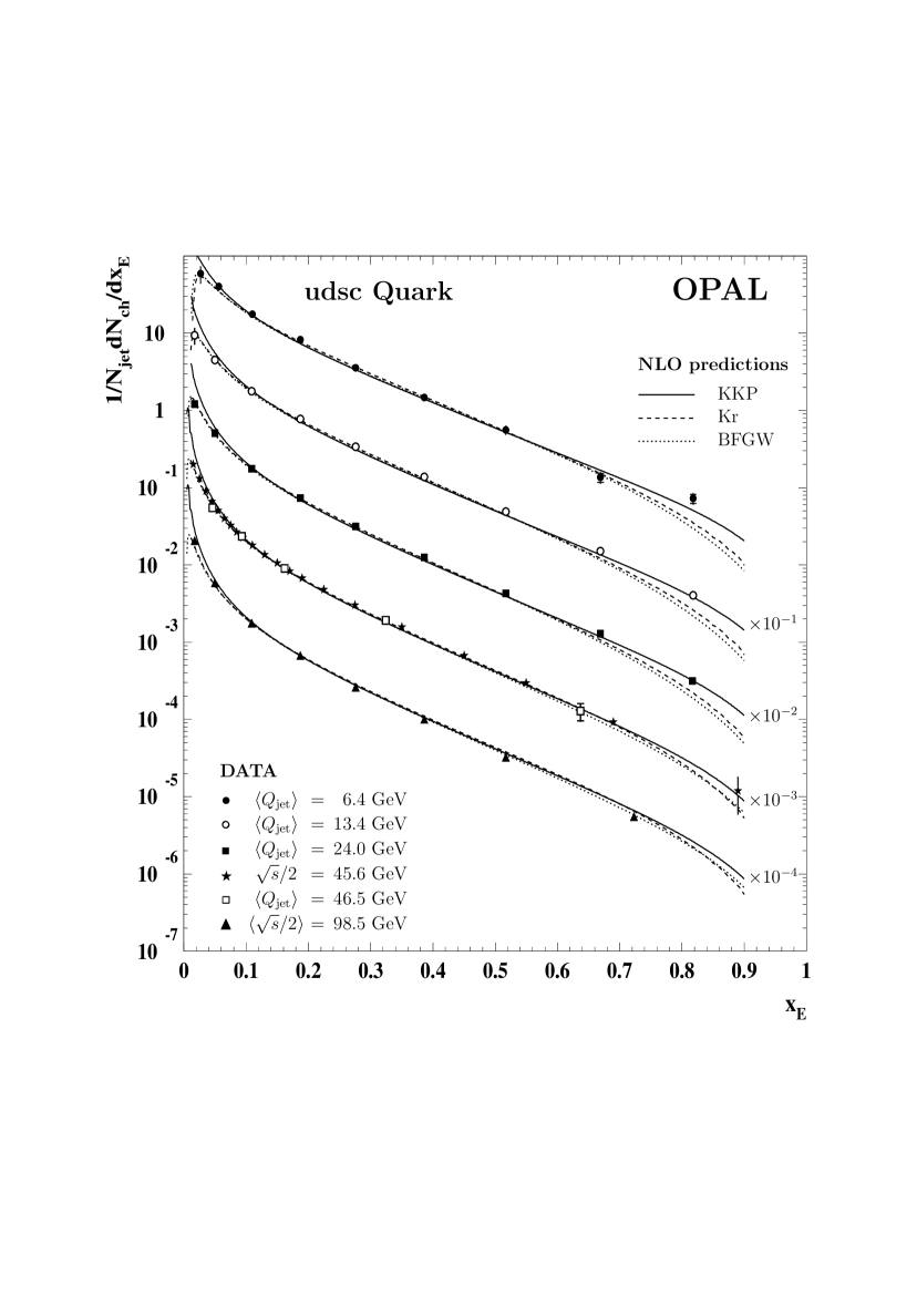
Figure 12: $x_{\mathrm{E}}$ dependence of the udsc jet fragmentation functions at different scales. The inner error bars indicate the statistical uncertainties, the total error bars show the statistical and systematic uncertainties added in quadrature. The values are given in Table 7. The data are compared to the NLO predictions by KKP [17], Kr [18] and BFGW [19]. The results are scaled as indicated in figure.

References

-
[1]
S.J. Brodsky and J.F. Gunion, Phys. Rev. Lett. 37 (1976) 402;
K. Konishi, A. Ukawa and G. Veneziano, Phys. Lett. B78 (1978) 243. -
[2]
OPAL Collaboration, G. Alexander et al., Phys. Lett. B265 (1991) 462;
OPAL Collaboration, P. Acton et al., Z. Phys. C58 (1993) 387;
OPAL Collaboration, R. Akers et al., Z. Phys. C68 (1995) 179;
DELPHI Collaboration, P. Abreu et al., Z. Phys. C70 (1996) 179;
ALEPH Collaboration, D. Buskulic et al., Phys. Lett. B384 (1996) 353. - [3] ALEPH Collaboration, D. Buskulic et al., Phys. Lett. B346 (1995) 389.
- [4] OPAL Collaboration, G. Abbiendi et al., Eur. Phys. J. C11 (1999) 217.
- [5] DELPHI Collaboration, P. Abreu et al., Eur. Phys. J. C13 (2000) 573.
- [6] S. Catani et al., Phys. Lett. B269 (1991) 432.
-
[7]
UA1 Collaboration, G. Arnison et al., Phys. Lett. B122 (1983) 103;
J.E. Huth et al., Snowmass (1990), Ed. E.L. Berger, World Scientific, Singapore (1990) 134;
OPAL Collaboration, R. Akers et al., Z. Phys. C63 (1994) 197. -
[8]
TASSO Collaboration, Z. Phys. C 47 (1990) 187;
MARK II Collaboration, A. Peterson et al., Phys. Rev. D37 (1998) 1;
TPC Collaboration, H. Aihara et al., Phys. Rev. Lett. 61 (1988) 1263;
AMY Collaboration, Y.K. Li et al., Phys. Rev. D41 (1990) 2675. - [9] DELPHI Collaboration, P. Abreu et al., Eur. Phys. J. C5 (1998) 585.
- [10] OPAL Collaboration, K. Ackerstaff et al., Eur. Phys. J. C7 (1999) 369.
-
[11]
CLEO Collaboration, M.S. Alam et al., Phys. Rev. D46 (1992) 4822;
CLEO Collaboration, M.S. Alam et al., Phys. Rev. D56 (1997) 17. -
[12]
OPAL Collaboration, G. Alexander et al., Phys. Lett. B388 (1996) 659;
OPAL Collaboration, K. Ackerstaff et al., Eur. Phys. J. C1 (1998) 479. - [13] OPAL Collaboration, G. Abbiendi et al., Eur. Phys. J. C23 (2002) 597.
- [14] OPAL Collaboration, G. Abbiendi et al., hep-ex/0310048, in press in Phys. Rev. D.
- [15] Yu.L. Dokshitzer, G.D. Leder, S. Moretti and B.R. Webber, JHEP 9708 (1997) 001.
-
[16]
V.N. Gribov and L.N. Lipatov, Sov. J. Nucl. 15 (1972) 438
and 675;
G. Altarelli and G. Parisi, Nucl. Phys. B126 (1977) 298;
Yu. L. Dokshitzer, Sov. Phys. JETP 46 (1977) 641. - [17] B.A. Kniehl, G. Kramer and B. Pötter, Nucl. Phys. B582 (2000) 514.
- [18] S. Kretzer, Phys. Rev. D62 (2000) 054001.
- [19] L. Bourhis, M. Fontannaz, J.Ph. Guillet and M. Werlen, Eur. Phys. J. C19 (2001) 89.
- [20] OPAL Collaboration, K. Ahmet et al., Nucl. Instr. Meth. A305 (1991) 275.
- [21] J. Allison et al., Nucl. Instr. Meth. A317 (1992) 47.
-
[22]
T. Sjöstrand, Comp. Phys. Commun. 82 (1994) 74;
T. Sjöstrand, CERN-TH 7112/93, revised August 1995. - [23] G. Corcella et al., JHEP 0101 (2001) 010.
- [24] OPAL Collaboration, G. Alexander et al., Z. Phys. C69 (1996) 543.
- [25] OPAL Collaboration, G. Abbiendi et al., Eur. Phys. J. C23 (2002) 597.
- [26] T. Sjöstrand, Comp. Phys. Commun. 135 (2001) 238.
- [27] S. Jadach, B.F.L. Ward and Z. Wa̧s, Comp. Phys. Commun. 130 (2000) 260.
- [28] L. Lönnblad, Comp. Phys. Commun. 71 (1992) 15.
- [29] ALEPH Collaboration, R. Barate et al., Phys. Rep. 294 (1998) 1.
- [30] J. Fujimoto et al., Comp. Phys. Commun. 100 (1997) 128.
- [31] OPAL Collaboration, G. Alexander et al., Z. Phys. C52 (1991) 175.
- [32] OPAL Collaboration, G. Alexander et al., Z. Phys. C72 (1996) 191.
- [33] OPAL Collaboration, K. Ackerstaff et al., Z. Phys. C75 (1997) 193.
- [34] OPAL Collaboration, G. Abbiendi et al., Eur. Phys. J. C16 (2000) 185.
- [35] OPAL Collaboration, G. Abbiendi et al., Eur. Phys. J. C27 (2003) 467.
- [36] R.K. Ellis, D.A. Ross and A.E. Terrano, Nucl. Phys. B178 (1981) 421.
- [37] S. Catani and M.H. Seymour, Phys. Lett. B378 (1996) 287.
- [38] ALEPH Collaboration, D. Buskulic et al., Z. Phys. C76 (1997) 191.
- [39] Yu. Dokshitzer et al., Basics of perturbative QCD, Editions Frontières (1991).
- [40] OPAL Collaboration, G. Abbiendi et al., Eur. Phys. J. C17 (2000) 373.
- [41] DELPHI Collaboration, P. Abreu et al., Phys. Lett. B449 (1999) 383.
- [42] OPAL Collaboration, G. Abbiendi et al., Eur. Phys. J. C8 (1999) 217.
-
[43]
A. De Rujula, J. R. Ellis et al., Nucl. Phys. B138 (1978) 387;
R. K. Ellis, W. J. Stirling and B. R. Webber, Cambridge Monogr. Part.
Phys. Nucl. Phys. Cosmol. 8 (1996). - [44] OPAL Collaboration, G. Abbiendi et al., Eur. Phys. J. C26 (2003) 479.
- [45] OPAL Collaboration, G. Abbiendi et al., Phys. Lett. B493 (2000) 249.
- [46] Yu.L. Dokshitzer, V.A. Khoze and S.I. Troyan, J. Phys. G17 (1991) 1602.
- [47] P. Edén and G. Gustafson, JHEP 9809 (1998) 015.
- [48] Xing-Qi Lu, Ph.D. Thesis, John Hopkins University, 1986.
- [49] ALEPH Collaboration, R. Barate et al., Eur. Phys. J.C17 (2000) 1.
- [50] UA1 Collaboration, G. Bocquet et al., Phys. Lett.B286 (1987) 509.
-
[51]
M. Radici and R. Jakob, Fragmentation function database:
http://www.pv.infn.it/~radici/FFdatabase/. - [52] G.D. Lafferty and T.R. Wyatt, Nucl. Instr. and Meth. A355 (1995) 541.
-
[53]
OPAL Collaboration, R. Akers et al., Z. Phys. C61 (1994) 204;
OPAL Collaboration, G. Alexander et al., Phys. Lett. B352 (1995) 176;
OPAL Collaboration, R. Akers et al., Z. Phys. C68 (1995) 203;
SLD Collaboration, K. Abe et al., Phys. Lett. B386 (1996) 475;
OPAL Collaboration, G. Abbiendi et al., Phys. Lett. B550 (2002) 33.