Precision Measurement of $\sin^{2}\theta_{W}$ at a Reactor

Abstract

This paper presents a strategy for measuring $\sin^{2}\theta_{W}$ to $\sim$1% at a reactor-based experiment, using $\overline{\nu}e$ elastic scattering. This error is comparable to the NuTeV, SLAC E158, and APV results on $\sin^{2}\theta_{W}$, but with substantially different systematic contributions. The measurement can be performed using the near detector of the presently proposed reactor-based oscillation experiments. We conclude that an absolute error of $\sim\!\delta({\mathrm{sin}}^{2}\theta_{W})=0.0019$ may be achieved.

This paper outlines a method for measuring $\sin^{2}\theta_{W}$ $(Q^{2}\approx 0)$ at a reactor-based experiment. The study is motivated by the NuTeV result, a $3\sigma$ deviation of $\sin^{2}\theta_{W}$ from the Standard Model prediction Zeller et al. (2002), measured in deep inelastic neutrino scattering ($Q^{2}=$ 1 to 140 GeV², $\langle Q^{2}_{\nu}\rangle=26$ GeV², $\langle Q^{2}_{\overline{\nu}}\rangle=15$ GeV²). Various Beyond-the-Standard Model explanations have been put forward sam ; Davidson et al. (2002); Loinaz et al. (2003), and, to fully resolve the issue, many require a follow-up experiment which probes the neutral weak couplings specifically with neutrinos, such as the one described here.

This proposed measurement is also interesting as an additional precision study at $Q^{2}=4\!\times\!10^{-6}$ GeV². The two existing low $Q^{2}$ measurements are from atomic parity violation (APV) Bennett and Wieman (1999), which samples $Q^{2}\sim 10^{-10}$ GeV²; and SLAC E158, a Møller scattering experiment at average $Q^{2}=0.026$ GeV² Anthony et al. (2004). Using the measurements at the $Z$-pole with $Q^{2}=M_{z}^{2}$ to fix the value of $\sin^{2}\theta_{W}$, and evolving to low $Q^{2}$, Fig. 1 shows that these results are in agreement with the Standard Model. However, the radiative corrections to neutrino interactions allow sensitivity to high mass particles which are complementary to the APV and Møller scattering corrections. Thus, this proposed measurement will provide valuable additional information.

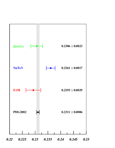
Figure 1: Measurements of $\sin^{2}\theta_{W}$, extrapolated to the $Z^{0}$ mass, from reference Anthony et al. (2004).

The technique we employ uses the rate of the purely leptonic $\overline{\nu}e$ scattering to measure $\sin^{2}\theta_{W}$. This signal was first detected by Reines, Gurr, and Sobel Reines et al. (1976), who measured $\sin^{2}\theta_{W}=0.29\pm 0.05$. In this paper, we explore what is necessary to improve on their idea and make a competitive measurement today. One important step is to normalize the $\overline{\nu}e$ “elastic scatters” using the $\overline{\nu}p$ inverse beta decay events, to reduce the error on the flux. Other crucial improvements are that the detector is located beneath an overburden of $\sim$300 mwe (meters, water-equivalent) and built in a clean environment. We find that a measurement of $\pm 0.0020$ is achievable. This is comparable to the NuTeV error of $\pm 0.00164$, and may help clarify the theoretical situation, as shown in references Rosner (2004); Loinaz et al. .

The proposed design employs spherical scintillator oil detectors similar to those used by CHOOZ Apollonio et al. (2003) and by other experiments which have been proposed to measure the oscillation parameter $\theta_{13}$ Anderson et al. (2004).

This style of detector has been optimized to reconstruct $\overline{\nu}p\to e^{+}n$ events, which dominate the rate when the reactor is running. We show that this design is also suitable for measuring $\sin^{2}\theta_{W}$ to high precision. Initially, one might think otherwise, since the $\overline{\nu}p$ events represent a potential background. However, this background can be controlled. In fact, these events are invaluable because they provide the normalization constraint. This normalization measurement must be done in the same detector as the $\overline{\nu}e$ measurement to exploit cancellations of systematics, especially those related to the fiducial volume.

To control backgrounds, this analysis exploits a visible energy ($E_{vis}$) “window”. We will show that we can obtain significant signal statistics even in this limited region. On the other hand, this range is above most environmental backgrounds in the detector, and below the energy produced by neutron capture in Gd.

This paper is organized in the following manner. In Sec. I, we identify the important questions which drive the design choices. In Sec. II, we provide details of the generic experiment and analysis used for estimates. In Sec. III, we discuss $\overline{\nu}e$ event identification and rates. In Sec. IV, we discuss rejection of $\overline{\nu}p$ events. In Sec. V, we consider backgrounds produced by natural radioactivity and cosmic rays. In Sec VI, we consider the errors on the $\overline{\nu}p$ normalization sample. In Sec. VII, we discuss how we find the error on $\sin^{2}\theta_{W}$. Finally, in Sec. VIII, we present our conclusions.

The goal of this paper is to establish that this analysis is worth pursuing at a reactor-based experiment. Thus the analysis is presented in sufficient detail to address what we have identified as the major issues. Many detailed studies remain to be done, however, as we discuss in the conclusions. In order to demonstrate feasibility we have relied on techniques for reducing background which are well-established in our determination of the error on $\sin^{2}\theta_{W}$.

I Introduction to the Design Issues

NuTeV has made a 0.72% measurement, including statistics and systematics, of the weak mixing angle. This error corresponds to a 1.15% uncertainty on the $\overline{\nu}e$ absolute rate at a reactor experiment. With this in mind, in order to establish the design for this experiment, the following questions must be explored:

1. Are there sufficient elastic scattering events to perform this measurement?

2. Can the elastic scattering events be isolated from the inverse beta decay events?

3. Can the environmental backgrounds be controlled?

4. How well can the anti-neutrino flux be known?

This section provides qualitative answers to establish that an error on $\sin^{2}\theta_{W}$ comparable to NuTeV is feasible.

This section also provides simple motivations for the major cuts. Briefly sketched, these are: a fiducial volume cut which is well within the Gd-doped region; vetoes for cosmics; an energy window cut; and a timing window to search for neutrons which follow a neutrino interaction. Here, we aim only to address the basic needs and challenges. The specifics on the cuts are described in Sec. II.2. The consequences of the cuts are explored in Sec.s III through VI.

Throughout the paper, we will identify certain backgrounds as “negligible.” We define negligible as a contribution to the total error of $\leq 0.1$%. In the case of backgrounds to the signal, this amounts to $<10$ events.

I.1 Statistics

Figure 2: Left: Comparison of $\overline{\nu}e$ (Elastic Scatters) and $\overline{\nu}p$ (inverse beta-decay) cross sections as a function of neutrino energy in MeV. Right: Comparison of event rates for $\overline{\nu}e$ and $\overline{\nu}p$ as a function of neutrino energy in MeV. Note that electron targets exceed free proton targets in the oil by a factor of 4.3.

The signal sample consists of elastic scattering events (“Elastic Sample”). A $\leq 1$% statistical error, corresponding to $\geq$10,000 elastic events, is necessary if the goal is a total error comparable to NuTeV.

The number of elastic scattering events and inverse beta decay events scale together. Since our premise is to use near detectors for the $\theta_{13}$ measurement, which utilizes inverse beta decay events, it is instructive to understand the relative rates of these two processes. Fig. 2 (left) compares the cross sections for these interactions as a function of neutrino energy in MeV, scaled for convenience. Fig. 2 (right) compares the unscaled number of events. At low energies, where $\overline{\nu}p$ is kinematically suppressed, elastic scattering dominates. Finally, Fig. 3 compares the absolute event rates as a function of visible energy in the detector. The elastic scattering events peak at low visible energy due to the energy carried away by the outgoing neutrino. From Fig. 3, one can see that if greater than $1\!\times\!10^{6}$ $\overline{\nu}p$ events can be collected in the visible energy window, then one will obtain more than $1\!\times\!10^{5}$ $\overline{\nu}e$ events. Thus the necessary statistical precision of $<1$% on elastic scattering can be reached.

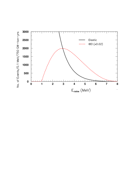
Figure 3: Visible energy distribution for inverse beta decay (red, dashed) and elastic scattering events (black, solid). Inverse beta decay events are scaled by a factor of 0.02 to allow visual comparison.

Based on this, we require a design which results in $>1\!\times\!10^{6}$ $\overline{\nu}p$ events. This goal is in concert with the requirements for a near detector for a $\theta_{13}$ measurement Anderson et al. (2004). The designs under consideration build on the past experience of the CHOOZ experiment, which observed $\sim$3000 inverse beta decay events in a 5 ton detector located 1 km from two 4.5 GW reactors, running for 132 days effective full power Apollonio et al. (2003). The proposed near detectors are typically located about 200 m from the reactor, gaining a factor of 25 from solid angle. The detector will be built with increased fiducial mass. Multiple detectors can be built. The experiment can feasibly run longer. In summary, the necessary event rate appears to be attainable with reasonable modifications to the CHOOZ setup.

I.2 $\overline{\nu}p$ Mis-identification

Inverse beta-decay events are a major component of the reactor-on rate in the proposed visible energy window. The best method for separating these events from elastic scatters is observation of the signal from neutron capture. This will motivate a fiducial volume cut which is well within the Gd-doped region to assure high efficiency for capturing the neutron. It will also motivate a data acquisition system which is sensitive to neutron capture on H, which occurs 16% of the time despite the Gd doping. Lastly, it will motivate an efficient time window for the neutron search. These are all discussed in detail in Sec. IV.

I.3 Environmental Backgrounds

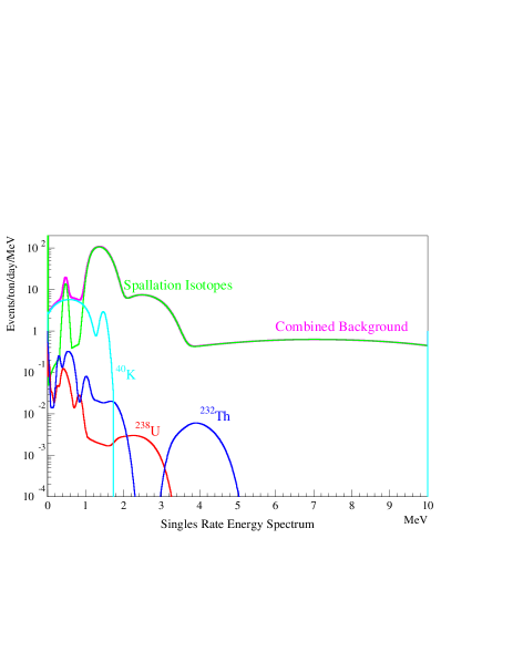
Figure 4: Simulated visible energy distribution and sources of singles events in a scintillation detector located at a depth of 300 mwe with a flat overburdon. The assumed isotope concentrations come from KamLAND Nakamura (2004).

Environmental backgrounds are by far the most important issue in the analysis and therefore deserve substantial introduction here. They fall into two categories: naturally occurring radioactivity and muon-induced backgrounds. To gain a sense of the background expectations, Fig. 4 shows a simulated visible energy spectrum for singles events consistent with Braidwood bra . The simulation assumes complete containment of all decay daughters, and uses an energy resolution of 7.5%/$\sqrt{E(MeV)}$, and a Birks’ constant of 0.00165 cm/MeV to quench the energy response to alphas. The naturally occurring radioactive contaminants mainly populate the low energy range of Fig. 4 and can, in part, be kept under control by maintaining KamLAND standards of oil purity, but, unlike KamLAND, this experiment will use Gd-doped scintillator, and so the Gd must also be purified of radioactive contaminants. The other source of environmental background, the $\beta$-decays of muon-induced (or “spallation”) isotopes, populate the higher energy range of Fig. 4.

To reduce background from radioactivity, we introduce spatial and energy cuts. Activity from the tank walls, the phototubes, and the acrylic vessel separating the Gd-doped and undoped regions can be removed by a strong fiducial volume cut. Most background from radioactivity dissolved in the scintillator can be removed from the sample through a $3<E_{vis}<5$ MeV cut on visible energy, as seen in Fig. 4. However,the ²³²Th chain produces ²⁰⁸Tl, which $\beta$-decays in our visible energy window and must be addressed.

Potential background from cosmic rays comes from 1) the muons themselves; 2) electrons from muon decays (“Michel electrons”); 3) ¹²B decays from $\mu^{-}$ capture; 4) spallation neutrons; and 5) isotopes generated by the high energy muons. The first four are straightforward to reduce. The fifth is, potentially, the most significant background in this analysis.

First, consider the four which are straightforward. Muons which enter the tank can be easily identified by means of the large energies which they deposit. Muons which stop may decay to produce electrons, or capture to produce ¹²B, which $\beta$-decays. The need to identify stopping muons motivates a veto based on a combination of tank hits and lack of hits in a hodoscope below the tank. Neutrons which are produced in combination with a cosmic ray event will be identifiable by their capture. Spallation neutrons which are unassociated with a cosmic ray have two sources. They may be produced outside of the tank and then enter; or they may be produced by high energy muon interactions with the ¹²C in the tank, but not be associated with the parent cosmic due to a late capture time. The Gd-doped buffer region surrounding the fiducial region provides further protection from incoming neutrons. We will show that the proposed visible energy window eliminates unassociated neutrons in the tank.

Isotope	Source
9Li	${}^{12}{\rm C}+\mu\rightarrow 3{\rm p}+^{9}{\rm Li}+\mu$
8He	${}^{1}2{\rm C}+\mu^{-}\rightarrow{\rm d}+{\rm 2p}+^{8}{\rm He}$; ${}^{12}{\rm C}+\mu\rightarrow{\rm 4p}+^{8}{\rm He}+\mu$
8Li	${}^{12}{\rm C}+\mu\rightarrow{\rm 3p}+{\rm 1n}+^{8}{\rm Li}+\mu$
6He	${}^{12}{\rm C}+\mu\rightarrow\alpha+{\rm 2p}+^{6}{\rm He}+\mu$
9C	${}^{12}{\rm C}+\mu\rightarrow{\rm 3n}+^{9}{\rm C}+\mu$
8B	${}^{12}{\rm C}+\mu\rightarrow{\rm 3n}+{\rm 1p}+^{8}{\rm B}+\mu$
12B	${}^{12}{\rm C}+n\rightarrow p+^{12}{\rm B}$

Table 1: Examples of sources of isotopes which $\beta$ decay producing potential background to this analysis.

Production mechanisms for the fifth source, $\beta$-decaying isotopes produced by high energy muons, are listed in Table 1. These isotopes are the dominate contribution to the singles rate above 3 MeV, as indicated by the “Spallation Isotope” curve in Fig. 4. These are ⁹Li, ⁸He, ⁸Li , ⁹C , ⁸B, ¹²B, all of which have endpoints above 10 MeV; and ⁶He, which has an endpoint of 3.5 MeV. ¹¹Be is not considered in the standard analysis because its muon induced production has only been reported as an upper limit Hagner et al. (2000). However, we do consider the case where this contribution is equal to the limit as an alternate scenario in Sec. VII.

The most important and straightforward way to reduce the rates of these isotopes is to have a large overburden. In addition a veto system is also employed. The veto system must be more elaborate than a simple rejection of events following an incoming cosmic ray, because the long half-lifes of the isotopes results in an intolerable deadtime with this configuration. However, a veto which identifies the subset of parent cosmics with evidence of an accompanying hadronic shower results in a tolerable deadtime. This is called a muon-hadron veto, and is described in Sec. V.1.5. This veto is the only proposed cut which is not based on past experience.

I.4 Normalization

Absolute knowledge of the reactor neutrino flux is limited to $\sim$2% due to uncertainties on the reactor power and fuel composition. To avoid this systematic, we use $\overline{\nu}p$ events (the “Normalization Sample”) to establish the normalization for the $\overline{\nu}e$ events. The statistical error on the $\overline{\nu}p$ events is small since more than $1\!\times\!10^{6}$ events are expected. The cross section for $\overline{\nu}p$ is well known from theory, as discussed in Sec. IV, so the systematic error from this source is negligible. An important systematic error comes from determination of the ratio of targets for $\overline{\nu}e$ versus $\overline{\nu}p$ scatters, i.e. the electron-to-free-proton ratio. Another important systematic question is related to neutron identification. One can obtain a very pure sample of $\overline{\nu}p$ events by requiring a Gd capture. This, however, will introduce a systematic error from the ratio of Gd captures to the total. This error was 1% in CHOOZ. This is unacceptably high for this analysis and must be reduced through improved calibration studies. Alternatively, assuming the trigger has high efficiency for events with H captures, one can accept all $n$-identified events into the $\overline{\nu}p$ sample. This eliminates the error on the Gd capture ratio but introduces possible backgrounds from accidental coincidences. Estimating these backgrounds will require a detailed study, beyond the scope of the present work. Therefore, for this analysis, we will use the former method of identifying a clean sample through the Gd captures.

II The General Design and “Standard” Analysis Cuts

Days of running:	900 Days
Number of reactor cores:	2
Power of each core:	3.6 GW
Overburden:	300 mwe
Distance to near detectors:	224 m
Number of near detectors:	2
Number of far detectors:	4

Table 2: Overview of general assumptions

To calculate an expected error on $\sin^{2}\theta_{W}$, we must make assumptions about the design. A summary of the assumptions is presented in Table 2. The setup is drawn from an preliminary design of the Braidwood $\theta_{13}$ experiment bra . The site has two 3.6 GW reactors which are assumed to produce a neutrino flux consistent with reference Bemporad et al. (2002). The model for this study uses two near detectors, located 224 m from the reactors, and four far, which are located 1.8 km away (here the far detectors are used only to measure backgrounds). All six detectors are assumed to be identical spherical vessels with both active and passive shielding. Data taking is assumed to extend over 900 live-days.

Basic Detector Design Parameters
Radius of fiducial region	150 cm
Fiducial volume per detector	13 tons
Outer radius of central region	190 cm
Tonnage of the central region	26.5 tons
Outer radius of photon catcher	220 cm
Outer radius of detector	290 cm
Path lengths of Particles (for Containment)
e- and e+ track length	negligible
e+ to n separation length (for $\overline{\nu}p$ events)	6 cm
0.5 MeV $\gamma$ Compton path length	11 cm
Neutron Parameters (for ID Efficiency)
Fraction of n which capture on Gd (H)	84% (16%)
Neutron capture time	30.5 $\mu$s

Table 3: Assumptions related to the detector design used in this paper.

It is necessary to make some specific assumptions in order to proceed with our calculations. These choices are reasonable and so serve for the proof-of-principle calculation. Small variations of this “generic” plan are expected and can easily be accommodated. Table 3 summarizes the assumptions. We address 1) basic definition of detector regions, 2) assumptions about track length which are relevant to calculating backgrounds, and 3) parameters related to identification efficiency which are relevant for calculating both backgrounds and the normalization rate.

II.1 The Basic Detector Design

The outer radius of the detector design is chosen to allow the detectors to fit in a 3 m radius tunnel. The interior sizes are scaled to match this requirement. The detector has a “central region” of Gd-doped scintillator, a “photon catcher” region which surrounds this, and an “oil buffer” region which separates the active regions from the phototubes and tank walls. For the sake of this discussion, we take the outer radius of the central region to be 190 cm. The fiducial region must be of substantially smaller radius to maximize containment of the neutrons produced by $\overline{\nu}p$ events and minimize environmental backgrounds. We will assume a fiducial radius of 150 cm. The Gd-doped region is surrounded by a 30 cm “photon catcher” of scintillator with no Gd doping. The photon catcher permits high efficiency for observing the 0.5 MeV $\gamma$’s produced by annihilation in $\overline{\nu}p$ events. These two regions are, in turn, surrounded by an oil “buffer” in which the phototubes are immersed. The buffer region extends out to a 290 cm radius. Hence the buffer is 70 cm in thickness and phototubes are located about 100 cm from the central region or 140 cm from the fiducial region.

Given this layout, the fiducial volume of each detector contains 13 tons. Therefore, two near detectors are required to attain the necessary statistics. This is consistent, for example, with the Braidwood Experiment design bra .

II.1.1 Response to Reactor-induced Events

The goal of the detector is to identify and count the two types of reactor-induced events: elastic scattering and inverse beta decay. In order to do this, accurate energy and vertex reconstruction are required. Also, it is necessary to identify neutrons produced in inverse beta decay with high efficiency. It is worth noting that, for this analysis, it is not necessary to reconstruct the angle of the outgoing lepton. This is in keeping with the detector design, where the the high level of scintillation light will obscure any directional Cerenkov light.

The two types of events have different visible energy distributions (Fig. 3), so to relate the rates for the two processes, one needs a good understanding of the energy resolution of the detector. Based on previous experiments, an energy resolution of $\leq$10% appears to be attainable Apollonio et al. (2003); Smirnov (2000); Eguchi et al. (2003). In Sec. VI, we show that systematics on smearing due to energy resolution leads to a negligible systematic error in the analysis whereas the uncertainty on energy calibration is significant.

Figure 5: Compton length in CH₂ as a function of photon energy.

To obtain good energy resolution for the normalization sample, the annihilation photons in inverse beta decay events must be contained. These photons lose energy through Compton scatters, with a path length that depends on energy and in CH₂, which is $\sim$11 cm at 0.5 MeV (see Fig. 5). While the Compton peak is at $2/3E_{\gamma}$, note that the average energy loss is $1/3E_{\gamma}$. Thus an event can be expected to have several Compton scatters before exiting the detector. The “photon catcher” region and outer 40 cm of the Gd-doped region are used to contain and reconstruct the energy of these photons. The 1.5 m radius fiducial volume cut places a 0.5 MeV photon at approximately 6.5 path lengths from the inactive oil-buffer region. The result is negligible loss due to escaping photons.

We do not consider vertex resolution smearing at the edge of the fiducial region. Instead, we assume that the relative vertex resolution is the same for the $\overline{\nu}e$ signal and $\overline{\nu}p$ normalization events to within 1 mm. Hence, the systematics related to vertex resolution cancel. We note that good vertex resolution is important for identifying and removing backgrounds. We believe that $\sim$4 cm on the interaction vertex may be attainable. This is consistent with CHOOZ laser flasher studies Apollonio et al. (2003). CTF obtained a similar resolution using an alpha source, corresponding to a photon energy of 0.862 MeV Smirnov (2000). This is sufficiently good that we believe vertex resolution issues will be a small effect in the final analysis and they are not considered further here.

To identify $\overline{\nu}p$ events, which represent both a background and a normalization sample, the signal from the neutron capture is used. In Gd-doped scintillator, a typical separation length from neutrino vertex to neutron capture is 6 cm, as measured in CHOOZ Apollonio et al. (2003). Therefore, the fiducial volume cut of 40 cm from the central region edge represents 6.7 separation lengths. Only a small fraction of the neutrons are produced at the edge of the fiducial region, and, of those, only about half drift outward. Folding in the geometry, assuming a uniform distribution for neutron production throughout the tank, $1.1\!\times\!10^{-5}$ of the neutrons will exit without capturing. This contribution to the background will be considered further in Sec. IV.

Neutron capture is delayed with respect to the positron track, with a mean capture time of 30.5 $\mu$s (as measured by CHOOZ Apollonio et al. (2003)). Using this as our baseline, we assume a neutron capture time window of $Deltat<200\mu$s. Based on our Monte Carlo (see Sec. II.3), this results in a failures to associate the neutron capture with the parent event $0.1$% of the time due to late captures. We address how these events can be removed in Sec. IV.

Neutron capture on Gd results in a cascade of photons with 5.6 to 8 MeV of deposited energy, depending on the Gd isotope. The dominant cross sections are for ¹⁵⁵Gd and ¹⁵⁷Gd, both of which result in $\sim$8 MeV of released energy. The remaining Gd isotopes represent $<9\!\times\!10^{-5}$ of all Gd captures. Those which released less than 6 MeV (¹⁵⁸Gd and ¹⁶⁰Gd) represent only $1.4\!\times\!10^{-5}$ of all Gd captures. Therefore we assume that the reconstructed energy for neutron captures on Gd is always $>5$ MeV.

CHOOZ found that the percentage of events which capture on Gd is 84% Apollonio et al. (2003). We use this capture fraction in our calculations. To increase the probability of Gd capture, it may be preferable to use isotopically-enhanced Gd. This has not been done in past experiments and requires further investigation.

The remaining 16% of neutrons will capture on hydrogen, resulting in a single 2.2 MeV $\gamma$. In this analysis, it is necessary for a large fraction of these events to be identified using a combination of timing and position. CHOOZ studied a trigger Baldini et al. (1997) for the H capture events, but this was developed late in the experiment and not implemented before data taking ended. However, the initial results looked promising. KamLAND quotes an efficiency for $\overline{\nu}p$ events of 78$\pm$1.6% Eguchi et al. (2003). This experiment is performed on oil with no Gd-doping, thus the neutron path length is large. The inefficiency is largely driven by the cut on relative position of the neutrino and neutron vertex. In order to proceed with background calculations, we assume a search window of 30 cm or five neutron path lengths will be feasible. This yields a 0.6% inefficiency due to neutrons which exit the window, which we will consider in Sec. IV. It is desirable to make this window larger, if the trigger rate can be tolerated.

II.1.2 Measuring the Gd and H Capture Fractions

CHOOZ measured the capture fraction on Gd with a 1% error using an Am/Be triggered neutron source. Because this experiment will run for three times the CHOOZ period, and because the Gd capture fraction can be measured in both near detectors and the four far detectors (see Sec. V.2), more than an order of magnitude more calibration data will be collected. Thus, in principle, the Gd capture fraction can be measured to better than 0.25%.

As additional assurance that the capture fraction can be measured well, we propose a small, dedicated detector with excellent energy resolution to accurately measure the fraction of Gd captures. The detector must have excellent energy resolution assuring a clean separation between the H capture energy peak and the Gd capture energy peak. The detector will consist of Gd doped scintillator which is of the same batch as the near and far detectors. A permanently installed Am/Be source would provide the trigger. One would want the fiducial radius to be at least six neutron path lengths, or 36 cm. It need not be a miniature version of the near detector – in fact other designs may be preferable and easy to obtain. For example, the SciBath detector design proposed by the FINeSSE experiment could be used for this purpose Bugel et al. (2004).

II.1.3 Contamination in the Detector

As discussed in Sec. I, the main decay chain of concern is ²³²Th. We will show in Sec. V that the fiducial volume cut reduces the background from the tank walls, phototubes, and acrylic vessel to a negligible level. Nevertheless, precautions at the level of KamLAND should be taken with these components.

The most important contamination issue is the amount of Th dissolved in the oil. A small fraction of the daughters in the ²³⁸U decay chain also produce visible energy in the 3 to 5 MeV region. Other radioactive contaminants, such as ⁴⁰K and ¹⁴C are not considered because the visible energy from these decays is below the energy level of this study. The far detectors will be used to study contaminants, so all detectors will be filled with oil from the same batch to assure consistent purity.

Our goal is to achieve the same fractional Th concentration in the scintillator as has been achieved at KamLAND Nakamura (2004), which is $5.2\!\times\!10^{-17}$ g/g. While we will show in Sec. VII.3 that two orders of magnitude higher contamination can be tolerated if necessary, KamLAND level purity is undoubtedly desirable. Reaching this level of purity requires addressing the cleanliness of the scintillator oil and also the contamination of the Gd-dopant. Purifying scintillator to attain low levels of dissolved thorium has been demonstrated. On the other hand, additional study is needed to assure the required purity of the Gd, which is isolated from contaminants by an evaporation process. For this discussion we assume that $5\!\times\!10^{-17}$ g/g of ²³²Th can be attained in the detector, although we will show that 100 times this rate can be tolerated.

Our goal for ²³⁸U contamination is the KamLAND level of $3.5\!\times\!10^{-18}$ g/g Nakamura (2004). The issue of contamination of the Gd must be addressed to achieve these goals.

II.1.4 Cosmic Ray Identification Systems

As described in Sec. I, cosmic ray background must be reduced for this analysis. For our assumed overburden we calculate a cosmic ray flux, of 0.5 $\mu$/m²/s or 3.5 Hz/detector.

For the oscillation experiment, most designs propose an active veto region which surrounds the detector Link (2003). This can be designed with at least $>99.99$% efficiency as achieved in MiniBooNE Aguilar-Arevalo et al. (2003).

For the purpose of identifying cosmic rays in the tank, we assume that 200 photoelectrons (PE) are detected per MeV of energy deposited in the detector. This rate of PE/MeV is similar to the CHOOZ design Apollonio et al. (2003) and is one third less than the Borexino test detector, CTF Alimonti et al. (1998). It is more than sufficient for our needs here.

Cosmic rays in the detector are the unique source of events above the Michel electron cutoff (about 52 MeV), and are, therefore, easily identifiable. Cosmic ray muons deposit about 2 MeV/cm Aguilar-Arevalo et al. (2003); Groom et al. (2001). This yields 0.4 PE/cm/phototube for muons. For this analysis, we are interested in muons which penetrate into the fiducial volume. To penetrate into the fiducial region, the muons must pass through a minimum of 70 cm of scintillator, depositing 140 MeV of energy in this model, well above the Michel electron cutoff. We will call a muon with $E>140$ MeV a “penetrating $\mu$” for the remainder of the discussion.

The need to simultaneously reconstruct reactor-induced events and penetrating $\mu$’s implies that the electronics must be sufficient to reconstruct events which range from 1 MeV to at least 140 MeV. Ability to resolve energies above 140 MeV is desirable, since it will allow better understanding of the cosmic rays. With 200 PE/MeV and 1000 phototubes, 140 MeV represents 28 PE/phototube. Thus, the electronics requires a minimum dynamic range of at least a factor of $\sim$30 (i.e. from 1 PE to more than 28 PE) without saturation. The electronics used in SNO Newcomer and Van Berg (1995) had a dynamic range of 1 to 1000 PE, so a substantially larger range is certainly possible.

The absence of a hit in the lower portion of the veto can be used to select events where the muon stopped in the detector. This will reduce the rate of potential parent cosmic rays for the ¹²B search to an acceptable level and also allow this source to be isolated for calibration. This veto system should be segmented, so that when used in conjunction with the upper veto, the cosmic ray track direction can be reconstructed to within a few centimeters. This also reduces false coincidence rates.

II.2 The Standard Cuts

Cuts, all samples	Range Retained	Primary Motivation
Fiducial volume	45 cm inward from Gd boundary	maintain high $n$ efficiency.
Vetoes, all samples	Description	Primary Motivation
Stopping Muon Veto	No lower veto hit & penetrating $\mu$;	vetoes 12B & Michel $e^{-}$
	veto window: 260 ms	(deadtime: 1.9%)
Muon-Hadron Veto	Through-going $\mu$ with more energy than expected	vetoes isotopes which $\beta$-decay
	from ionization or a neutron capture within 600 ms;	(deadtime: 4.2%)
	veto window: 3 s
Cuts, elastic scattering sample	Range Retained	Primary Motivation
Minimum visible energy	$>3$ MeV	Reduce all sources
Maximum visible energy	$<5$ MeV	of backgrounds
Neutron capture energy	$<1.8MeV$	identify and cut $\overline{\nu}p$
& delay window	$\Delta T<200\mu$s
Cuts, normalization sample	Range Retained	Primary Motivation
Neutron capture energy	$E>5$ MeV	Isolate well-identified events to
& delay window	$\Delta T<200\mu$s	maximize $n$ id purity
Minimum visible energy	$>2.2$ MeV	isolate events with flux which
		overlaps $\overline{\nu}e$ signal

Table 4: General motivation for the major cuts. “Elastic” and “Normalization” samples are described in Sec. I. Visible energy refers to the measured energy of the primary interaction.

Based on the detector described above, we propose a set of analysis cuts. These will be used to evaluate the capability of the experiment. The cuts fall into four categories: cuts applied to both event samples; vetoes applied to all event samples; cuts applied to isolate the elastic scattering sample; and cuts applied to isolate the normalization sample. The standard cuts on which we will base our estimate for the error on $\sin^{2}\theta_{W}$ are listed in Table 4.

II.2.1 Overview of Analysis Level Vetoes

Two analysis-level vetoes are employed: the stopped muon veto and the muon-hadron veto. The first veto is designed to reduce background from Michel electrons and ¹²B beta-decays. The second removes high-energy-muon-induced $\beta$-decaying isotopes.

The stopped muon veto is applied in the following way. The presence of a “stopped muon” is identified by requiring a penetrating $\mu$ in coincidence with no exiting signal in the lower veto system. All subsequent events in a 260 ms window are then eliminated. The 260 ms window was chosen because it is about twelve times the ¹²B half-life and thousands of muon lifetimes. It thereby effectively eliminates the stopped $\mu$ backgrounds.

For this discussion, we will assume the stopped muon veto is 100% efficient. Inefficiency in identifying the muon signal could cause this veto to fail. However, this is expected to be negligible. Inefficiency in the lower veto increases the deadtime, as discussed below, but does not cause the veto to fail. Noise in the lower veto in coincidence with a stopping cosmic could cause the veto to fail. But a combination of selecting quiet phototubes and segmented construction can reduce this to a negligible level.

The muon-hadron veto removes all events in a 3 second window following a though-going muon accompanied by either a significant energy deposition over that expected from ionization alone, or at least one captured neutron within 600 ms. The purpose is to reduce the background from muon-induced $\beta$-decaying isotopes. The production of these isotopes is typically accompanied by a sizable hadronic shower and an average of 3 free neutrons Wang et al. (2001) (in many cases the neutrons are fragments of the parent ¹²C isotope, see Table 1). For the purposes of this study we assume that the muon-hadron veto will be 95% efficient.

II.2.2 Deadtime Induced by the Vetoes

Deadtime is not a major consideration in this analysis because the signal and normalization samples will be equally affected. Nevertheless, when one is performing a precision measurement, as a matter of practice it is best to have the lowest possible deadtime. Also, one aims for a small deadtime so that one can run for the minimum possible time. In considering the discussion below, note that a veto which depends only on the presence of a cosmic ray, without asking for a stopping signal or accompanying hadronic activity, would lead to intolerable deadtimes.

The deadtime for the stopped muon veto will be 1.1% given the expected stopped muon rate of 0.042 Hz. This is acceptable. In principle, inefficiency in the lower veto could produce misidentified stopping muons. It is reasonable to assume that this veto can be made better than 99% efficient. Assuming a 1% inefficiency would lead to a deadtime of only 1.9% (veto inefficiency and real stopped muon rate, combined). This is sufficiently small that it is not an issue.

To calculate the rate at which the muon-hadron veto will fire, one needs to consider both the muon rate and the neutron capture rate. To estimate the neutron rate, we use a simulation which is described in Sec. II.3. We expect 0.042 muon-induced neutrons/s. However, we note that many of these neutrons will be produced in association with the same cosmic muon. To correct for multiple neutron production, we use the calculated average multiplicity of three. Thus we take as our prediction a rate of 0.014 Hz. Opening a 3 s window, thereby introduces a 4.2% deadtime. This is an acceptable rate and is probably an overestimate. In fact, to further reduce backgrounds from $\beta$-decaying isotopes, one might consider enlarging this window.

To address the rate of accidental firing of this veto, we must consider the types of events which can cause each component to fire. The cosmic signal is unique among the types of events which can occur, due to the very high energy. Therefore, we assume that there is no accidental background in this component. The most likely false vetoes come from Michel electrons and ¹²B decays, because these events are correlated with an incoming muon. Neutrons which enter the tank can also produce a muon-neutron coincidence. This rate is much lower, however, because the neutron and cosmic ray are not correlated, and so we do not consider this here.

II.3 Calculation of Neutron Production and Transport

The above discussion and that which follows relies on a simulation of the interactions of cosmic rays muons at the expected overburden. To calculate the production of fast neutrons we begin with a parameterization of the muon rate at the surface as a function of energy and zenith angle Hagiwara et al. (2002). The muon rate is divided into 750,000 bins in energy (100 MeV steps from 0 to 2.5 TeV) and angle ($2^{\circ}$ steps from $0^{\circ}$ to $60^{\circ}$). In each bin the energy is attenuated over steps of one meter (larger steps are used for very high energies) according to the average energy loss as a function of muon energy Groom et al. (2001). The muon rate and spectrum at the given depth are used to determine the neutron spectrum and rate following the neutron production model of Wang et al. Wang et al. (2001) . Similarly, the isotope production is determined using the normalization and energy scaling of Hagner et al. Hagner et al. (2000). The production rates for ⁹Li, ⁸He, ⁸Li, ⁶He, ⁹C, and ⁸B come from the measured rate of Hagner et al., and the ¹²B rate comes from an observation made by KamLAND Araki et al. (2004).

The neutron transport Monte Carlo takes the neutron production energy distribution as an input, and propagates the neutrons assuming elastic scattering in $CH_{2}$ with 0.1% Gd by weight. The cross sections for elastic scattering and capture on H, C, and Gd are taken from reference Garber and Kinsey (1976). These calculations are then used in determining the efficiency of the muon neutron veto and inverse beta decay rejection.

III $\overline{\nu}e$ Event Rate and Identification

Neutrino-electron scattering measurements have been studied for many years Imlay and VanDalen (2003). $\overline{\nu}e$ events result either from scattering via exchange of a $Z$ boson, or annihilation via exchange of a $W$ boson. The differential cross section for $\overline{\nu}_{e}e^{-}$ scattering is:

$$\frac{d\sigma}{dT}\! \!=\! \!\frac{\pi\alpha^{2}\mu_{e}^{2}}{m_{e}^{2}}\frac{\left(1-T/E_{\nu}\right)}{T}+\frac{G_{F}^{2}m_{e}}{2\pi}\times$$

$$\!\left[\left(g_{V}\!+\!g_{A}\right)^{2}\!+\!\left(g_{V}\!-\!g_{A}\right)^{2}\!\left(\!1\!-\!\frac{T}{E_{\nu}}\!\right)^{2}\!+\!\left(g_{A}^{2}\!-\!g_{V}^{2}\right)\!\frac{m_{e}T}{E_{\nu}^{2}}\!\right]$$

where $E_{\nu}$ is the incident $\overline{\nu}_{e}$ energy, T the electron recoil kinetic energy, and the couplings are given by Vogel and Engel (1989)

$$g_{V}=2\sin^{2}\theta_{W}+\frac{1}{2}\text{~{}~{}~{}~{} }g_{A}=-\frac{1}{2}.$$

The term in brackets is the weak interaction contribution, and the last term gives the contribution from electromagnetic scattering if the neutrino has a magnetic moment, $\mu_{e}$.

The total visible energy, $E_{vis}$ in elastic scatters is the kinetic energy of the $e^{-}$, $T$. This is in contrast to $\overline{\nu}p$ events where additional visible energy will come from both the positron annihilation and the neutron capture.

If one could reconstruct both $T$ and $E_{\nu}$ in $\overline{\nu}e$ events, then an analysis of the $T/E_{\nu}$ dependence would be attractive. This method evades the issue of absolute normalization. However, in the generic detector described above the angle of the $e^{-}$ cannot be reconstructed. Therefore, only $T$ is measurable. Once this cross section is folded with the reactor flux, the variation of the shape versus $T$ is insensitive to $\sin^{2}\theta_{W}$.

On the other hand, the total rate of $\overline{\nu}$ events is sensitive to $\sin^{2}\theta_{W}$. In fact, the sensitivity to $\sin^{2}\theta_{W}$ can be enhanced by introducing a cut on $T$. Integrating over the recoil electron kinetic energy from $T_{\min}$ to $T_{\max}$ gives a cross section as a function of $E_{\nu}$ given by:

$$\sigma\mid_{T_{\min}}^{T_{\max}} =\frac{G_{F}^{2}m_{e}}{2\pi}\!\left[\!\left(\left(g_{V}\!+\!g_{A}\right)^{2}+\left(g_{V}\!-\!g_{A}\right)^{2}\right)\left(T_{\max}\!-\!T_{\min}\right)\right.$$

$$+\frac{1}{2}\!\left(\frac{m_{e}\left(g_{A}^{2}\!-\!g_{V}^{2}\right)}{E_{\nu}^{2}}\!-\!\frac{2\left(g_{V}\!-\!g_{A}\right)^{2}}{E_{\nu}}\right)\!\left(T_{\max}^{2}\!-\!T_{\min}^{2}\right)$$

$$\left.\!+\!\frac{\left(g_{V}\!-\!g_{A}\right)^{2}}{3E_{\nu}^{2}}\left(T_{\max}^{3}\!-\!T_{\min}^{3}\right)\right]$$

$T$ in the range of 2.5 to 5 MeV is optimal. As discussed in Sec. I, however, cuts on various backgrounds dictate $3<(T=E_{vis})<5$ MeV.

We assume that the term associated with the neutrino magnetic moment ($\mu_{e}$) is negligible, based on astrophysical constraints Fukugita and Yazaki (1987); Lattimer and Cooperstein (1988); Barbieri and Mohapatra (1988); Raffelt (1999). We note, though, that the lab-based limits on the neutrino magnetic moment are two orders of magnitude higher Daraktchieva et al. (2003). If the neutrino magnetic moment were just below the lab-based limit (e.g. $10^{-10}$), then this term would result in a 12% increase in the elastic scattering rate.

IV The $\overline{\nu}p$ Background

A major potential source of background comes from misidentified $\overline{\nu}_{e}p\rightarrow e^{+}n$ events. The cross section is given by Vogel and Beacom (1999):

$$\sigma\left(E_{e^{+}}\right)=\frac{2\pi^{2}}{m_{e}^{5}f\tau_{n}}p_{e^{+}}E_{e^{+}}$$

where $E_{e^{+}}(p_{e^{+}})$ is the energy(momentum) of the outgoing positron, $f=1.71465(15)$ Bemporad et al. (2002); Apollonio et al. (2003) is the free neutron decay phase-space factor, and $\tau_{n}=886.7\pm 1.9$ s Wilkenson (1982) is the neutron lifetime. Using these measurements of $f$ and $\tau_{n}$, one finds that the cross section is known to $\sim$0.2%. For this process, the $E_{\overline{\nu}_{e}}$ energy threshold is 1.804 MeV and the incoming $\overline{\nu}_{e}$ energy is simply related to the outgoing positron energy by

$$E_{\overline{\nu}}=E_{e^{+}}+(M_{n}-M_{p})=E_{e^{+}}+1.2933\text{ MeV}~{}.$$

Most $\overline{\nu}p\rightarrow e^{+}n$ are identified by the outgoing neutron. However, the neutron may not be observed, because of the the inefficiency on triggering on H capture, or because the neutron was outside of the neutron-delay time window. In the latter case, $0.1$% of the neutrons will capture late, leaving a primary neutrino vertex and a secondary neutron vertex which is mistakenly unassociated. However, the $E_{vis}$ window requirement further reduced the fraction of these events that contribute to as background to the $\overline{\nu}e$ sample.

IV.1 Rejection through $n$ Identification

Most $\overline{\nu}p$ events can be rejected through identification of the time-delayed $n$. We take the efficiency for reconstructing the photons from Gd capture to be 100%. On the other hand, the efficiency for identifying the photon associated with H capture is only $99.4$%. Thus the total $n$-identification efficiency is $0.84+(0.16\times 0.994)=0.999$. This is to say, $0.1$% of $n$ events within the neutron time window will fail to be identified.

The systematic error on this is small. The error on the Gd capture fraction is assumed to be 0.3% (see Sec. II). The Gd capture fraction introduces an error, $\delta$, which changes the efficiency to $\epsilon=(0.84+\delta)+(0.16-\delta)\times 0.994$. Therefore $d\epsilon=0.006\times d\delta\simeq 2\!\times\!10^{-5}$. From binomial statistics, one needs only 17,000 tagged calibration-source events to obtain a 10% error on this inefficiency. This should be achievable using the in situ Am/Be source calibration. We therefore assume no systematic error contribution from this source.

IV.2 Rejection through an $E_{vis}$ Cut

There are three cases where the neutron is “lost” to the analysis. First, the neutron capture occurs outside the neutron delay time window in 0.1% of the cases. Second, $0.0011$% of the time the neutron exit the Gd-doped central region without capturing. Third, for $0.1$% of the time the neutron captures on hydrogen, but it is outside the H-trigger spatially allowed range (see Sec. II.1.1). The rates for these potential sources of background are all further reduced by the $E_{vis}$ cut.

In each of these cases only the positron energy is observed. Approximately 45% of the positron events fall within the $E_{vis}$ MeV window. The background for late captures is, therefore, 0.045% of all $\overline{\nu}p$ interactions. The fraction of events with a neutron which exit and with neutrino vertex energy in the window is $7\!\times\!10^{-6}$. The case where the neutron is lost from the H-trigger search region, follows the same argument. This background source is, therefore, 0.045% of the $\overline{\nu}p$ events. Again we assume no appreciable systematic error on these values.

Based on this, we estimate the the total $\overline{\nu}p$ background to be 0.09% of the $\overline{\nu}p$ interactions with a negligible systematic error.

V Environmental Backgrounds

Section I introduced the environmental backgrounds which reactor experiments face. Potentially, they come from contaminants, cosmic ray muons, and products of cosmic ray muons such as Michel electrons, spallation neutrons, and muon-produced isotopes. We assume cosmic muons are readily identifiable, as described in Sec. II.1.4. We show that the $3<E_{vis}<5$ MeV window, in combination with the vetoes proposed in Sec. II.2.1, reduce most environmental backgrounds to a negligible level.

V.1 Sources

V.1.1 ²³⁸U and ²³²Th decay chains

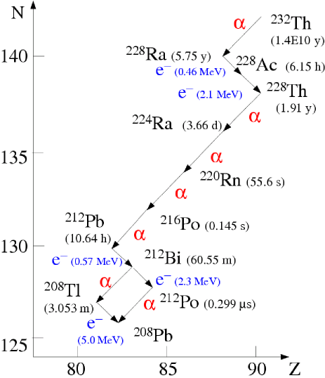
Figure 6: Decay chain for ²³⁸Th. The half-life of each step is listed in parentheses. For $\beta$ decays, the total visible energy released ($\beta$’s and $\gamma$’s) is noted.

The decay chain for ²³²Th is shown in Fig. 6. The half-life for each step is also listed in the figure.

The ²³²Th chain produces six alpha particles of energy 4 to 9 MeV. Scintillation signals quench by a factor of 10 to 15, so each alpha deposits roughly 0.25 to 0.8 MeV in the detector. It is highly unlikely that multiple decays will occur simultaneously, thus the $\alpha$’s do not represent a background.

Five $\beta$’s are also produced in the decay chain, and the respective energies of the $\beta$’s are listed on Fig. 6. The issue for this analysis is the decay of ²⁰⁸Tl to ²⁰⁸Pb. This releases a $\beta$ with energy up to 1.8 MeV and, simultaneously, $\gamma$’s, including a 2.4 MeV $\gamma$. The total energy of this decay is 5 MeV. Therefore this decay has sufficient energy to appear in the $3<E_{vis}<5$ MeV window. This decay lies on a branch of the chain, such that only 35% of the parent ²³²Th will result this decay.

The Th-related contaminants on the acrylic vessel will not result in background because the events will be removed by the fiducial volume requirement for this analysis. Also, any $\gamma$’s produced by this decay chain, which may enter the fiducial volume, will be below the 3 MeV visible energy window, which means that they will not contribute. Therefore, we only consider the ²³²Th dissolved in the scintillator.

Calculating from our assumed ²³²Th concentration of $5\!\times\!10^{-17}$ g/g, and half-life of $1.4\!\times\!10^{10}$ years we expect to have 183 decays of each isotope in the chain between the two detectors. But only 35% of the chains go through the ²⁰⁸Tl branch, and only 51% of those will have a visible energy on the 3 to 5 MeV window. Therefore, we expect only 93 ²³²Th background events in all.

As seen in Fig. 4, there is also a small fraction of background events, from 3 to 3.5 MeV, which are due to the ²³⁸U chain. These events are produced from a $\beta$ decay within this chain with an endpoint of 3.2 MeV. We will assume that we can achieve the same level of uranium contamination as KamLAND. Judging from Fig. 4, the U contribution in the visible energy window is only about 5% of the Th contribution, or about 5 events for the two near detectors combined.

The systematic error on these backgrounds can be determined by two methods. In the first method, samples of the oil will be studied in a low background counting facility located deep underground. This will allow a precise absolute measure of the $\beta$ decay of concern. However, it relies on Monte Carlo to accurately represent the smearing. In the second method, the far detectors are used to measure the background expected in the near detector. This method is discussed in Sec. V.2.

V.1.2 Michel Electrons

The ratio of stopping to through-going muons at 300 mwe has been calculated to be $6\!\times\!10^{-3}$/m Cassiday et al. (1973). The flux of cosmic rays entering a detector under 300 mwe overburden is 0.5 $\mu$/m²/s. The stopping rate in the detector is therefore 0.042 Hz, or about $3.3\!\times\!10^{6}$ Michel decays per detector for the run.

The stopped muon veto represents many thousands of muon lifetimes, and so the background from Michel electrons is negligible in this analysis. Instead, Michel electrons represent a well-identified control sample for studies in this analysis. If all detectors are built identically, then the Michel samples can be combined, greatly enhancing these studies.

V.1.3 Neutrons

Cosmic rays can produce spallation neutrons either outside or within the tank, but these are a negligible background. This is because these neutrons, like unassociated neutrons described above, will fail the energy window. H captures result in a visible energy which is below 3 MeV, and Gd captures result in a visible energy above 5 MeV. Moreover, for neutrons which enter the tank, the $n$ must traverse 6.7 interaction lengths (40 cm) of Gd-doped scintillator in order to reach the fiducial volume. The resulting rejection is about 0.001. We therefore take this background to be negligible in this study.

V.1.4 Stopping-muon-induced ¹²B

Cosmic ray muons entering the detector may capture and produce ¹²B which $\beta$ decays. Capture occurs 8% of the time in oil Suzuki et al. (1987). Because only the $\mu^{-}$ captures, we gain a factor of two. In addition, only 19% of these events, appear in the $E_{vis}$ window, and only about 17% of $\mu^{-}$ captures on carbon result in the ground state of ¹²B Suzuki et al. (1987); Miller et al. (1972). Therefore, the rate of ¹²B decays from $\mu^{-}$ capture is about $5\!\times\!10^{-5}$ Hz. This represents about 4,000 events per detector during the run, which is too high a level of background for this analysis. To reduce the rate further, we introduced the stopping muon veto, which was described in Sec. II.2.1. The 260 ms veto window is about twelve times the half-life of ¹²B. We expect less than one ¹²B background events from $\mu^{-}$ capture between the two near detectors.

V.1.5 High-energy-muon-induced Isotopes

Isotope	Half-life	Endpoint	Rate	Rate
	(s)	(MeV)	(/t/d)	(detector/d)
9Li+8He	0.18 & 0.12	13.6 & 10.6	0.15$\pm$0.02	1.95$\pm$0.26
8Li	0.84	16.0	0.28$\pm$0.11	3.64$\pm$1.43
6He	0.81	3.5	1.1$\pm$0.2	14.70$\pm$2.60
12B	0.02	13.4	4	50
9C	0.13	16.0	0.34$\pm$0.11	4.42$\pm$1.43
8B	0.77	13.7	0.50$\pm$0.12	6.50$\pm$1.56

Table 5: Isotopes with energy endpoint $>3$ MeV. Rate/detector/day is for the generic 13 ton detector under 300 mwe overburden. Top table: $\beta^{-}$ production; bottom table: $\beta^{+}$ production.

High energy cosmic rays produce $\beta$ decaying isotopes in a number of ways. Spallation refers specifically to nuclear disintegration due to interaction with a virtual photon, although the term is often used loosely. Other sources are elastic and inelastic scattering. High energy secondary neutrons and pions can also produce isotopes, so that modeling the transport and interaction of secondaries is important. Calculations using measured isotope production rates by muons are in fairly good agreement with the observations at KamLAND and can thus be used to estimate the background rates for this measurement. The sources for muon-induced $\beta$-decaying isotopes of particular concern for this analysis are listed in Table 1.

The raw rates for a 13 ton fiducial volume scintillator-oil-based detector located under a 300 mwe overburden are shown in column 5 of Table 5.

The signal from ⁹Li and ⁸He were indistinguishable in the NA54 data Hagner et al. (2000), and hence they are grouped together here. For the sake of argument here, we assume that the contributions of ⁹Li and ⁸He are equal for the measured rate in NA54, although we consider this further below. It should be noted that if the relative rates of the two processes are not determined, then one needs to include a systematic which covers the range from the assumption of 100% Li to 100% He.

Isotope	$E_{vis}$ Cut	Correlated $n$	Veto/Final Rate
9Li	0.18	0.09	0.0045
	(19%)	(50%)	(5%)
8He	0.29	0.24	0.012
	(30%)	(84%)	(5%)
8Li	0.47	N/A	0.024
	(13%)		(5%)
6He	0.29	N/A	0.015
	(2%)		(5%)
12B	9.5	N/A	0.48
	(19%)		(5%)
9C	0.53	N/A	0.027
	(12%)		(5%)
8B	0.65	N/A	0.033
	(10%)		(5%)

Table 6: Isotopes decays/detector/day after each cut, applied sequentially. Value in parenthesis is the percent of the rate retained after the cut.

By taking the fraction of events in a 3 to 5 MeV window, assuming the correct $\beta$-decay spectrum, we obtain the approximate rate with the energy cut, shown in Table 6, column 2. At the time of the $\beta$ decay, a neutron accompanies 50% of the ⁹Li decays and 16% of the ⁸He decays and therefore will not contribute to the elastic scattering background. One therefore obtains the rates shown in column 3. Finally, in column 4, we show the result of introducing the muon-hadron veto. The total is 0.60$\pm$0.13 (sys) events/day/detector or 1080$\pm$234 events in both detectors for the entire run. This leads to a systematic error of just over 2% in the 10000 event signal, which is at least a factor of two higher than can be accepted if the goal is to match the NuTeV errors. Therefore, it is crucial to constrain this systematic from the data.

V.1.6 Neutrino Backgrounds

Solar neutrinos also represent a possible environmental background. As calculated by reference Naples , the background from solar neutrino interactions is small. The rate for the flux between 3 to 5 MeV, which is expected to be dominated by the ⁸B solar neutrinos, is 4 events in the 900 day run. Atmospheric neutrino rates are considerably lower than solar neutrino rates, and so these, too, can be neglected. Also, geoneutrinos from $\beta$-decays in the core of the earth, which have energies $<2.6$ MeV, are not an issue in this analysis.

V.2 Use of the Far Detectors to Reduce the Systematic Error

The far detectors are an ideal place to cross check the predictions for environmental backgrounds, because the signal is less than 5% of the background rate in the far detectors. These backgrounds mainly come from muon-induced isotopes, but there is also a small contribution of from the ²³⁸U and ²³²Th contaminants.

The far detector measurements can constrain the near detector backgrounds only to the extent that all detectors are built identically. The design feature which is likely to be least similar between the near and far detectors is the overburden. Despite the homogeneity of the rock in, for example, the Braidwood area bra , the overburden for the near and far detectors may well differ by a few percent for shafts of identical depth.

With an overburden difference of $\sim$3%, the rate of muon-induced isotopes will differ in the near and far detectors. However, for such small variations in overburden, one expects shifts in the normalization, with no significant deviation as a function of energy. We propose two methods for correcting the muon-induced background normalization between the near and far detectors.

The first method is to correct the normalization in the far detector using the ratio of cosmic ray rates in the near compared to the far detectors. Given a cosmic ray rate of 3.5 Hz per detector, one expects more than $3\!\times\!10^{8}$ cosmic ray events per year in each detector. The statistical error in the normalization correction is therefore negligible. We will assume that this is the method which is employed, and not consider an error from the normalization correction.

The second method uses the high energy ($E>10$ MeV) $\beta$-decays to normalize the near-to-far detector rates. This cut is chosen to be sufficiently high so that in the near detector, inverse beta decay, and elastic scattering events do not contaminate the sample. It is sufficiently low, however, that we expect about 12,000 events per detector, allowing a high statistics measurement. It should be noted that this sample is not contaminated by Michel electrons due to the stopping muon veto. Given two near detectors we expect 24,000 events. The error on the normalization from this method is consequently about 0.6%. This is sufficiently small to serve as a useful cross check for the correction based on relative cosmic ray rates. Note that all of the isotopes except for ⁶He and ⁸He contribute to $E>10$; this is therefore a direct check of the dominant sources of isotopes.

The reactor-induced events in the far detector must be subtracted. At 1.8 km from the reactor core, the signal rate and the $\overline{\nu}p$ backgrounds are both reduced by the factor $(0.2/1.8)^{2}\simeq 0.01$. One therefore expects only about 50 elastic signal events and 13 inverse beta decay background per detector, compared to over 540 events from the environmental backgrounds.

Combining the information from all four far detectors, and then combining this with the direct calculation of Sec. V.1.5, 1080$\pm$32(stat)$\pm$23(sys) events.

From all sources of environmental backgrounds (U/Th and muon-induced isotopes) we expect a total of 1178$\pm$39(stat)$\pm$26(sys) events.

V.3 Comment on Overburden

	25 mwe	50 mwe	300 mwe	450 mwe
muons (/m2/s)	88.3	24.6	0.53	0.19
neutrons (/t/d)	11360	4942	322	145
9Li+8He	5.3$\pm$0.9	2.3$\pm$0.3	0.15$\pm$0.02	(6.6$\pm 0.7)\!\times\!10^{-2}$
8Li	10.$\pm$5.	4.4$\pm$1.9	0.28$\pm$0.11	0.13$\pm$0.05
6He	40.$\pm$12.	17.$\pm$4.5	1.1$\pm$0.2	0.50$\pm$0.07
12B	150	60	4	1.8
9C	12.1$\pm$5.3	5.2$\pm$2.1	0.34$\pm$0.11	0.15$\pm$0.05
8B	17.9$\pm$6.4	7.7$\pm$2.5	0.50$\pm$0.12	0.22$\pm$0.05

Table 7: Isotopes with energy endpoint $>3$ MeV for various overburdens. Rate for the isotopes is in decays/ton/day.

In this study we have assumed an overburden of 300 mwe equivalent. However, at the Braidwood site bra it is possible to reach 450 mwe. Larger overburden is advantageous to this analysis. The core-to-detector distance increases by $\sim$10%, but the rate of isotope production drops by more than a factor of two (see Table 7). As a result, 300 mwe should be regarded as a minimum and the detector halls will be constructed with the maximum feasible overburden.

If this experiment is performed at a facility where the overburden between near and far detectors varies substantially, so the far detector cannot be used to constrain the near detector background rates, then an overburden which is deeper than 300 mwe is recommended. One can use the $E>10$ MeV rates in the near detector to somewhat constrain the errors, but this does not significantly reduce the 2% error from the spallation background. With an overburden of 450 mwe one could achieve an error of $\sim$1%, which is not ideal but still tolerable.

On the other hand, a shallow overburden cannot be tolerated due to the high cosmic ray rate as shown in Table 7. For example, for 50 mwe, the through going cosmic ray rate increases by almost a factor of 15. The stopping rate will be substantially larger. This will lead to intolerable backgrounds from ¹²B and high-energy-muon-induced isotopes.

VI The $\bar{\nu}p$ Normalization Sample

Figure 7: Illustration of method for extracting the $\overline{\nu}_{e}$ flux. Top: inverse beta decay events vs. neutrino energy. Middle: predicted cross section for inverse beta decay events. Bottom: extracted flux obtained from dividing the event distribution by the predicted cross section.

Figure 8: Illustration of method for comparing elastic scattering interaction prediction to data. Top: elastic scattering cross section for interactions with visible energy between 3 and 5 MeV, for arbitrary $\sin^{2}\theta_{w}$, shown as a function of neutrino energy. Middle: resulting predicted event rate when the cross section (top) is multiplied by the flux distribution (Fig. 7, bottom). Bottom, bold: Rebinning of predicted event rate as a function of $E_{vis}$. Dotted line shows how the prediction would extend beyond the energy window. This predicted distribution will be compared with data.

The $\sin^{2}\theta_{W}$ measurement requires that the absolute $\overline{\nu}_{e}$ flux be known with good accuracy. The flux can be measured in a straightforward manner using the high statistics sample of $\overline{\nu}p$ inverse beta-decay events. This process is illustrated in Fig. 7. There is a one-to-one correspondence between visible energy and neutrino energy for these events:

$$E_{\nu}=E_{vis}+1.8-2m_{e}~{}.$$

As shown in Fig. 7 (top), therefore, the events can be binned as a function of $E_{\nu}$. The $\overline{\nu}p$ inverse beta-decay cross section, shown in Fig. 7 (middle), is very well known, both in shape and magnitude, from measurements of the neutron lifetime. This has an uncertainty of 0.2%. As a result, the flux can be extracted for neutrinos above the threshold energy for inverse beta decay, see Fig. 7 (bottom). This is the same flux which contributes to our signal events.

To extract the predicted number of signal events, we use the procedure illustrated by Fig. 8. The top plot in this figure shows the cross section for elastic scattering events with 3 to 5 MeV visible energy as a function of $E_{\nu}$. Multiplying this cross section by the flux in Fig. 7 (bottom), results in a total number of elastic scattering events with the visible energy cut, binned as a function of true $E_{\nu}$. This distribution is shown in Fig. 8 (middle). To see this, we rebin these events according to $E_{vis}$ and we obtain Fig. 8 (bottom). This distribution is the prediction which will be compared with data.

We will then vary $\sin^{2}\theta_{W}$ in the cross section, Fig. 8 (top), to obtain the best agreement between data and prediction. While the sensitivity is expected to mainly rely on normalization, the shape comparison will provide an important cross check.

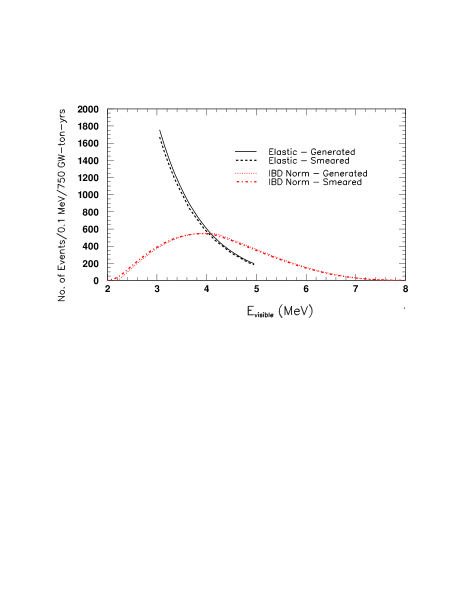
Figure 9: Comparison of generated and smeared visible energy distributions. Solid, Black: elastic scattering, generated; Dashed, Black: elastic scattering, smeared; Dotted, Red: inverse beta-decay generated; Dot-dashed, Red: inverse beta-decay smeared. The inverse beta-decay events (IBD Norm) have been weighted by the elastic to inverse beta-decay cross section ratio.

The error in the $\overline{\nu}e$ event prediction as a function of $\sin^{2}\theta_{W}$ has contributions from statistical and systematic uncertainties. The statistical uncertainty is related to the $\overline{\nu}p$ inverse beta-decay event sample used to determine the flux. For the assumed “generic experiment” described here, there are about $2.7\!\times\!10^{6}$ $\overline{\nu}p$ inverse beta-decay events which, when weighted by the cross section ratio of $\overline{\nu}_{e}e$ to $\overline{\nu}p$ interactions and Gd capture fraction, yields an effective number of $1.58\!\times\!10^{6}$ events. As a result, the statistical error associated with the flux normalization and energy dependence is very small due to the high statistics, giving a contribution of 0.08%.

Figure 10: Change in number of elastic scattering events versus energy resolution factor.

The elastic scattering events have a substantially different visible energy distribution, as compared to the inverse beta-decay events after weighting by the elastic to inverse beta-decay cross section ratio (Fig. 9). The reconstructed energy resolution smearing will therefore affect the two distributions differently, and a correction will need to be applied when using the inverse beta decay events for the elastic event prediction. Assuming an energy resolution of $\Delta E/E=0.07/\sqrt{E(MeV)}$, the number of elastic scattering events in the $3<E_{Visible}<5$ MeV region goes down by 5%, but the sum over the full region of the weighted inverse beta decay events changes very little, as seen in Fig. 9. One therefore needs to make a correction using a Monte Carlo simulation of the smearing and apply it to the prediction. This correction will depend on knowing the energy resolution for the detector. Fig. 10 shows the fractional change in the predicted number of elastic scattering events versus the energy resolution factor $k$ used in the parameterization, $\Delta E/E=k/\sqrt{E(MeV)}$. Sources and other types of calibrations will be used to determine $k$ for the experiment. For now, it is assumed that $k=0.07$ with an uncertainty of 10% or $\pm 0.007$. As seen from Fig. 10, this gives a systematic error on the normalization of 0.1% due to the uncertainty in $k$. This is negligible for the analysis.

Similarly, but more importantly, an energy scale error or an energy offset error will also affect the elastic scattering and inverse beta decay samples differently. Thus this systematic error does not effectively cancel. There are a number of ways to constrain energy scale and offset errors. The best method uses the large sample of ¹²B decays, which are $\beta$ decay events. If one can justify the conversion from photon to electron response, then one can also use the millions of reconstructed 2.2 MeV photons from neutron capture on Hydrogen. The peak at 4.9 MeV from capture on Carbon also offers a useful sample. In this paper, we assume a systematic error on the elastic scattering rate of 0.5% from energy scale or offset. This corresponds to knowledge of the energy scale to 0.33% or the offset to 7.5 keV. These are ambitious goals and clearly calibration is a high priority for the analysis.

There are important systematic errors associated with the number of free protons in the target and the number of electrons available as targets for elastic scattering. These systematic errors are correlated and the correlations need to be taken into account in calculating the normalization uncertainty. With this procedure the fractional error on the number of electrons is 75% of the error on the number of free protons. CHOOZ determined the number of free protons by burning their target material Apollonio et al. (2003), yielding a measurement accurate to 0.8%. Assuming we can do no better, the fractional error on the number of electrons is, therefore, 0.6%.

Another important systematic is the error on the fraction of neutrons which will be tagged by a Gd capture. As discussed in Sec. I, we use this sample because it selects events with negligible background. For a systematic error estimate, we assume that $84.00\pm 0.25$% events will capture on Gd.

VII Calculating the Error on $\sin^{2}\theta_{W}$

We first obtain the error on the number of signal events and then extract the error on $\sin^{2}\theta_{W}$. The terms which contribute to the error on the number of signal events are: 1) the statistical error on the signal; 2) the statistical and systematic errors associated with the $\overline{\nu}p$ background; 3) the statistical and systematic errors associated with the environmental backgrounds; and 4) the statistical and systematic errors associated with the normalization.

For the first calculation, we assume the standard set of proposed cuts. Next, we consider what is required to reach the NuTeV level of error. Then, we consider the impact if the experiment has less scintillator purity than proposed here. Lastly, we consider the impact if there is substantially more background from isotope decays than expected.

VII.1 Error on $\sin^{2}\theta_{W}$ for the Proposed Analysis

Statistical error on the signal	0.95%
Statistical error $\overline{\nu}p$ background subtraction	0.43%
Systematic error $\overline{\nu}p$ background subtraction	0.0%
Statistical error on U and Th background	0.09%
Systematic error on U and Th background	0.0%
Statistical error on muon-induced isotopes	0.33%
Systematic error on muon-induced isotopes	0.20%
Statistical error on the normalization	0.10%
Systematic error from energy scale/offset	0.50%
Systematic error on electron-to-free-proton ratio	0.60%
Systematic error on the Gd capture fraction	0.30%
Total error	1.40%

Table 8: Fractional errors contributing to the error on the number of $\overline{\nu}e$ scattering events based on assumptions presented in this paper. To equal the NuTeV error, 1.2% total error was required.

In this section, we consider the contribution of each error source. A summary of each of the sources, along with the fractional error on the number of $\overline{\nu}e$ events, is shown in Table 8. Where the contribution to the error was negligible ($<10$ events), we list 0% error.

The statistical error on the signal is calculated using the number of elastic scattering events in the $E_{vis}$ window, $N_{e}$. We find that for 900 days live-time, $N_{e}=11,400$ events.

The statistical error from the $\overline{\nu}p$ background subtraction is $\sqrt{N_{p~{}bkgd}}/N_{e}$, where $N_{p~{}bkgd}$ is the number of $\overline{\nu}p$ events passing the signal cuts. For 900 days live-time, we expect $N_{p}=2.70\!\times\!10^{6}$ $\overline{\nu}p$ events with a rejection efficiency of which only 2430 survive all cuts. We assume that the systematic error on the $\overline{\nu}p$ background measurement is negligible (see Sec. IV for justification).

The environmental backgrounds contribute both statistical and systematic errors. The statistical contribution is given by $\sqrt{N_{env}}$, and the contribution from the systematic error is $\sigma_{env~{}sys}/N_{e}$. We list the contribution from U and Th and muon-induced isotopes separately in Table 8. The systematic error on the ²³⁸U and ²³²Th contaminants is negligible but the systematic error on the muon-induced isotopes, $\pm$23 events, must be considered.

The statistical error due to the size of the normalization sample is very small, $\sim$0.08%, as described in Sec. VI. The first systematic error on the normalization comes from the uncertainty in the number of electrons in the sample, which is tied to the uncertainty in the number of free protons and is $dN_{target\ electrons}/N=0.6$%. The second significant systematic error on the normalization sample comes from the error on the knowledge of the Gd capture fraction. We have argued that 0.25% can be attained.

Adding the systematic errors in quadrature, we find $(dN/N)_{sys}=1.03$%. Adding this in quadrature with the statistical error on the signal yields $(dN/N)_{tot}=1.40$%. This is close to the goal of 1.15% which we set at the start of this paper. Extracting the error on $\sin^{2}\theta_{W}$, we obtain: $\delta(\sin^{2}\theta_{W})=0.0020$. This is comparable to the NuTeV error of 0.00164.

VII.2 Improving this Measurement

As one can see from Table 8, the error on $\sin^{2}\theta_{W}$ is dominated by statistics. If the running period were doubled to 1800 days, one would achieve $\delta(\sin^{2}\theta_{W})=0.0018$. Alternatives to increased running period include enlarging the detector, adding extra near detectors, finding a closer approach to the reactor cores, or moving to a more powerful reactor. Any of these options will incrementally improve the result.

The rate of production of muon-induced isotopes can be reduced by using a larger overburden. If the rate reduced by a factor of two by going to 450 mwe, then the error on $\sin^{2}\theta_{W}$ drops to 0.0019. If we have a 450 mwe overburden and the experiment runs for 1800 days, the experiment attains $\delta(\sin^{2}\theta_{W})=0.0017$. Reduction of these background events may also be achieved by a better muon-neutron veto. However, if the veto introduces excessive deadtime the loss in elastic scattering statistics may offset the gains in background reduction.

VII.3 Impact of Impurities of the Gd-Dopant

We have assumed that KamLAND levels of purity for U and Th ($5\!\times\!10^{-17}$ g/g Th) can be achieved. The techniques for purifying oil have been established by CTF and KamLAND and therefore appear to be practical. This experiment, however, requires that Gd dopant be added to the oil. Experience from CHOOZ Apollonio et al. (2003) indicates that this can introduce a high level of Th contamination, so purification of the Gd will need to be researched.

To establish the effect of increased contamination, consider the change in the error as the contamination is increased. In our calculation above, with 100 Th and U induced events in the $E_{vis}$ window, we achieved $\delta(\sin^{2}\theta_{W})=0.0020$. Two orders of magnitude increase in U and Th contamination gives $\delta(\sin^{2}\theta_{W})=0.0024$, which is within a tolerable range, especially given that running longer will still result in a substantial reduction in error. However, three orders of magnitude larger contamination renders the result uninteresting. This constrains the necessary level of purity which must be achieved to better than $5\!\times\!10^{-15}$ g/g of Th.

VII.4 Impact of Increased Isotope Background

We have calculated the background from $\beta$-decaying isotopes based on calculations from reference Hagner et al. (2000). We did not, however, include the background from ¹¹Be, for which only a gross upper limit has been set Hagner et al. (2000). Using this upper limit as an expected level of isotope production increases the background from 1458 to 1803 events. This produces a negligible shift in $\delta(\sin^{2}\theta_{W})$. In fact, increasing the total isotope background by a factor of two only increases $\delta(\sin^{2}\theta_{W})$ to 0.0021.

VIII Conclusions

This paper discusses a technique for measuring $\sin^{2}\theta_{W}$ at a reactor-based experiment using $\overline{\nu}e$ elastic scatters. A precise measurement of $\sin^{2}\theta_{W}$ at $Q^{2}\approx 4\times 10^{-6}$ GeV², neutrinos as probes opens a window for tests of neutrino properties and electroweak theory. We have used an experimental design which is consistent with many proposals for near detectors at reactor-based oscillation experiments. We have also assumed realistic reactor power and a human-scale run time of about 900 days.

The analysis has statistical and systematic errors which are roughly equal, so increased statistics will yield further improvement. At least $\sim$26 tons of fiducial volume are required and the detector should be located as close as possible to the reactor ($\sim$250 m or less).

We have also introduced the idea of normalizing to the $\overline{\nu}p$ events. This substantially reduces the error from the flux. Because the normalization sample is measured in the same detector as the elastic scattering signal, many systematics effectively cancel, including those associated with deadtime and fiducial volume.

We have also considered backgrounds from misidentified inverse beta decay events. Using $n$-identification and a visible energy window, this background can be reduced to an acceptable level. Environmental background is dominated by the contribution from spallation by cosmic ray muons which produce isotopes which $\beta$-decay. To attain acceptable rates, 300 mwe overburden is the minimum required. Indeed, deeper overburden is desirable. Future studies on reducing this background by identifying muons which cause spallation are important. It is also necessary to maintain oil and Gd purity from U and Th contaminants. Our calculations show that KamLAND-levels of purity are desirable, but an increase of two orders of magnitude of impurity is acceptable.

This exercise was meant to serve as a proof-of-principle that a reasonable error on $\sin^{2}\theta_{W}$ can be attained at a reactor-based experiment. The technique has not yet been fully optimized. The total error which we obtain on $\sin^{2}\theta_{W}$ is $\delta(\sin^{2}\theta_{W})$=0.0020. This is similar to the NuTeV error of 0.00164 and is lower than the published SLAC E158 and APV results. A measurement at this precision will uniquely probe the electroweak and neutrino sectors and is currently being explored by several groups Rosner (2004); Loinaz et al. . Based on this study, we conclude that the idea is feasible and more detailed studies are warranted.

Acknowledgments

We thank G. P. Zeller, H. Newfield-Plunkett and the Columbia Neutrino Group for their input. Also, we thank S. Biller, T. Bolton, J. Formaggio, K. Heeger, P. Fisher, G. Gratta, R. Imlay, W. Louis, D. Naples, P. Nienaber and P. Vogel for their comments.

References

- Zeller et al. (2002) G. P. Zeller et al. (NuTeV), Phys. Rev. Lett. 88, 091802 (2002), eprint hep-ex/0110059.
- (2) For a complete set of theoretical papers on this subject, see http://home.fnal.gov/gzeller/nutev.html.
- Davidson et al. (2002) S. Davidson, S. Forte, P. Gambino, N. Rius, and A. Strumia, JHEP 02, 037 (2002), eprint hep-ph/0112302.
- Loinaz et al. (2003) W. Loinaz, N. Okamura, T. Takeuchi, and L. C. R. Wijewardhana, Phys. Rev. D67, 073012 (2003), eprint hep-ph/0210193.
- Bennett and Wieman (1999) S. C. Bennett and C. E. Wieman, Phys. Rev. Lett. 82, 2484 (1999), eprint hep-ex/9903022.
- Anthony et al. (2004) P. L. Anthony et al. (SLAC E158), Phys. Rev. Lett. 92, 181602 (2004), eprint hep-ex/0312035.
- Reines et al. (1976) F. Reines, H. S. Gurr, and H. W. Sobel, Phys. Rev. Lett. 37, 315 (1976).
- Rosner (2004) J. L. Rosner, Submitted to Phys. Rev. D (2004), eprint hep-ph/0404264.
- (9) W. Loinaz, P. Fisher, and T. Takeuchi, paper in preperation.
- Apollonio et al. (2003) M. Apollonio et al., Eur. Phys. J. C27, 331 (2003), eprint hep-ex/0301017.
- Anderson et al. (2004) K. Anderson et al., White paper report on using nuclear reactors to search for a value of (2004), eprint hep-ex/0402041.
- Nakamura (2004) K. Nakamura (KamLAND), AIP Conf. Proc. 721, 12 (2004).
- (13) See http://braidwood.uchicago.edu.
- Hagner et al. (2000) T. Hagner et al., Astropart. Phys. 14, 33 (2000).
- Bemporad et al. (2002) C. Bemporad, G. Gratta, and P. Vogel, Rev. Mod. Phys. 74, 297 (2002), eprint hep-ph/0107277.
- Smirnov (2000) O. J. Smirnov, Tech. Rep. INFN/TC-00/17, INFN Gran Sasso (2000).
- Eguchi et al. (2003) K. Eguchi et al. (KamLAND), Phys. Rev. Lett. 90, 021802 (2003), eprint hep-ex/0212021.
- Baldini et al. (1997) A. Baldini et al., Nucl. Instrum. Meth. A389, 141 (1997).
- Bugel et al. (2004) L. Bugel et al. (FINeSSE), Tech. Rep. FERMILAB-PROPOSAL-937, Fermilab (2004), eprint hep-ex/0402007.
- Link (2003) J. M. Link, in Intersections of Particle and Nuclear Physics (2003), AIP 698, pp. 771–774.
- Aguilar-Arevalo et al. (2003) A. A. Aguilar-Arevalo et al. (MiniBooNE) (2003), the MiniBooNE Run Plan, available at http://www-boone.fnal.gov/publicpages/news.html.
- Alimonti et al. (1998) G. Alimonti et al. (Borexino), Astropart. Phys. 8, 141 (1998).
- Groom et al. (2001) D. E. Groom, N. V. Mokhov, and S. I. Striganov, Atom. Data Nucl. Data Tabl. 78, 183 (2001).
- Newcomer and Van Berg (1995) F. M. Newcomer and R. Van Berg, IEEE Trans. Nucl. Sci. 42, 745 (1995).
- Wang et al. (2001) Y. F. Wang et al., Phys. Rev. D64, 013012 (2001), eprint hep-ex/0101049.
- Hagiwara et al. (2002) K. Hagiwara et al. (Particle Data Group), Phys. Rev. D66, 010001 (2002).
- Araki et al. (2004) T. Araki et al. (KamLAND) (2004), eprint hep-ex/0406035.
- Garber and Kinsey (1976) D. I. Garber and R. R. Kinsey, Tech. Rep. Neutron Cross Sections, BNL325, Brookhaven National Lab (1976).
- Imlay and VanDalen (2003) R. Imlay and G. VanDalen, J. Phys. G29, 2647 (2003).
- Vogel and Engel (1989) P. Vogel and J. Engel, Phys. Rev. D39, 3378 (1989).
- Fukugita and Yazaki (1987) M. Fukugita and S. Yazaki, Phys. Rev. D36, 3817 (1987).
- Lattimer and Cooperstein (1988) J. M. Lattimer and J. Cooperstein, Phys. Rev. Lett. 61, 23 (1988).
- Barbieri and Mohapatra (1988) R. Barbieri and R. N. Mohapatra, Phys. Rev. Lett. 61, 27 (1988).
- Raffelt (1999) G. G. Raffelt, Phys. Rept. 320, 319 (1999).
- Daraktchieva et al. (2003) Z. Daraktchieva et al. (MUNU), Phys. Lett. B564, 190 (2003), eprint hep-ex/0304011.
- Vogel and Beacom (1999) P. Vogel and J. F. Beacom, Phys. Rev. D60, 053003 (1999), eprint hep-ph/9903554.
- Wilkenson (1982) D. Wilkenson, Nucl. Phys. A337, 474 (1982).
- Cassiday et al. (1973) G. L. Cassiday, J. W. Keuffel, and J. A. Thompson, Phys. Rev. D7, 2022 (1973).
- Suzuki et al. (1987) T. Suzuki, D. F. Measday, and J. P. Roalsvig, Phys. Rev. C35, 2212 (1987).
- Miller et al. (1972) G. Miller, M. Eckhause, F. Kane, P. Martin, and R. Welsh, Phys. Lett. 41B, 50 (1972).
- (41) D. Naples, private communication.