KEK Preprint 2004-1

KEK-TH-947

Higgs pair production at a linear $\bf e^{+}e^{-}$ collider
in models with large extra dimensions

Nicolas Delerue , Keisuke Fujii and Nobuchika Okada

High Energy Accelerator Research Organization (KEK)
1-1 Oho, Tsukuba, Ibaraki 305-0801, JAPAN

To be submitted to Physical Review Journal D, rapid communications

Abstract
In this paper, we will derive the cross section formula for the Higgs pair production at a linear $e^{+}e^{-}$ collider in models with large extra dimensions and study the feasibility of its measurement through realistic Monte Carlo simulations. Since the process has essentially no Standard Model background, once produced, it will provide us with a very clean signature of physics beyond the Standard Model. Moreover, since the final state particles are spinless, the spin 2 of the intermediate virtual KK gravitons has to be conserved by the orbital angular momentum of the Higgs pair. This results in a very characteristic angular distribution of the final states. Taking into account finite detector acceptance and resolutions as well as initial state radiation and beamstrahlung, we demonstrate in this paper that, given a sufficiently high center of mass energy, the angular distribution of the Higgs pair is indeed measurable at the linear collider and will allow us to prove the spin 2 nature of the KK gravitons exchanged in the $s$-channel.

1 Introduction

Large extra dimension scenario [1] provides an alternative solution to the gauge hierarchy problem, the huge hierarchy between the electroweak scale and the Planck scale, without supersymmetry. In this scenario, while keeping the four dimensional Planck scale as it is, we can bring the fundamental gravity scale down as low as to ${\cal O}$(1TeV), by the arrangement of the extra dimensional volume. For example, in the case of models with extra $\delta$ dimensions being compactified on a torus $T^{\delta}$ with a common radius $R$, the four dimensional Planck scale ($M_{4}$) is obtained through the Gauss law, $M_{4}^{2}\sim M_{4+\delta}^{2+\delta}R^{\delta}$, where $M_{4+\delta}$ is the $4+\delta$ dimensional Planck scale. Since all the standard model fields are assumed to be confined on the brane, the existence of the extra dimensions can be felt only through the very weak gravity interactions, and the models are found to be consistent with the current experiments even if $M_{4+\delta}\sim{\cal O}(1~{}\mbox{TeV})$ for $\delta\geq 2$ [2]. Of great interests is that this scenario is testable at colliders, and its collider signatures have been intensively investigated [3].

In the four dimensional description, there is an infinite tower of Kaluza-Klein (KK) modes of graviton, whose masses are characterized by the compactification radius and integers corresponding to quantization of momentum in the extra dimensional directions. The existence of the extra dimensions can be revealed through processes involving the KK mode gravitons at the colliders. There are two important types of processes. One involves direct emission of the KK gravitons. Since KK gravitons interact with the standard model fields very weakly, they are regarded as invisible stable particles. Such a process will thus appear as missing energy events at the colliders. The other comprises the processes mediated by virtual KK gravitons. In this case, new effective contact interactions will be induced in addition to the standard model interactions.

In this paper, we study the Higgs pair production process at a future linear $e^{+}e^{-}$ collider. This process has two interesting points to be stressed. Firstly, the Higgs pair production cross section at the linear collider is highly suppressed in the standard model. If the cross section mediated by the virtual KK gravitons is large enough, it will hence be a very clean signal of physics beyond the Standard Model. Secondly, the clean and well defined environment of the linear collider allows the measurement of the angular distribution of the final states, which carries information on the spins of the intermediate states. Being scalar particles, the produced pair of Higgs bosons will show a very characteristic angular distribution, since the spin 2 of the intermediate KK gravitons has to be conserved by the orbital angular momentum of the final states.

In the next section we will derive the cross section formula for this process and show this explicitly. Based on the derived formula, we will then carry out Monte Carlo simulations in Section 3 and demonstrate that we can indeed measure the angular distribution. The final section summarizes our results and concludes this paper.

2 Theoretical Framework

In this section, we will derive the cross section formula for the Higgs pair production. For simplicity, we assume the extra $\delta$ dimensions are compactified on the torus $T^{\delta}$ with a common radius $R$. In the four dimensional description, the interaction Lagrangian between the standard model fields and the KK gravitons ($G^{(\vec{n})}_{\mu\nu}$) or KK gravi-scalars ($H^{(\vec{n})}$) is then given by [7, 8]

$${\cal L}_{int}=-\frac{1}{{\bar{M}}_{p}}\sum_{\vec{n}}\left(G^{(\vec{n})}_{\mu\nu}T^{\mu\nu}+H^{(\vec{n})}T^{\mu}_{\mu}\right),$$ (1)

where $\vec{n}=(n_{1},n_{2},..,n_{\delta})$ with $n_{i}$’s being integers, $T_{\mu\nu}$ is the energy-momentum tensor of the standard model fields, and ${\bar{M}}_{p}=M_{4}/\sqrt{8\pi}$ is the reduced four dimensional Planck scale. The $n$-th KK mode mass squared is characterized by $m_{(\vec{n})}^{2}=|\vec{n}|^{2}/R^{2}$. Since the trace of the energy-momentum tensor is proportional to the mass of the fields under the field equations of motion, we neglect processes mediated by the KK gravi-scalars in our study for the linear $e^{+}e^{-}$ collider, and consider only the processes mediated by the KK gravitons.

In this setup, the scattering amplitude via the $s$-channel KK graviton exchange for a general 2-to-2 process, $e^{-}(p_{1})+e^{+}(p_{2})\rightarrow X(p_{3})+Y(p_{4})$, is found to be

$${\cal M}=\sum_{\vec{n}}\left(-\frac{1}{\bar{M}_{p}^{2}}\right)\frac{1}{s^{2}-m_{(\vec{n})}^{2}}T^{\mu\nu}(p_{1},p_{2})T_{\mu\nu}(p_{3},p_{4})$$ (2)

in momentum space. Note that there is a difficulty in this process (for $\delta\geq 2$), namely, the ultraviolet divergence according to the summation over the infinite tower of the KK modes. Unfortunately no one knows how to regularize the divergence because of the lack of knowledge about gravity theories at energies much higher than the ($4+\delta$ dimensional) Planck scale. In the following analysis, we naively introduce an ultraviolet cutoff for the highest KK modes, and replace the summation by [7]

$$\frac{4\pi}{M_{S}^{4}}=-\frac{1}{\bar{M}_{p}^{2}}\sum_{\vec{n}}\frac{1}{s-m_{(\vec{n})}^{2}},$$ (3)

where $M_{S}$ is the cutoff scale naturally being of the order of $M_{4+\delta}$. Our amplitude will then become

$${\cal M}=\frac{4\pi}{M_{S}^{4}}T^{\mu\nu}(p_{1},p_{2})T_{\mu\nu}(p_{3},p_{4}).$$ (4)

We use this formula for the collider’s center of mass energies below $M_{S}$.

Let us apply the framework given above to the Higgs pair production process, $e^{+}e^{-}\rightarrow HH$, mediated by the virtual KK gravitons. Only the free parts in the (physical) Higgs Lagrangian, the kinetic and the mass terms, contribute to this process. In this process, the energy momentum tensors in the amplitude are explicitly given by

$$T^{\mu\nu}(p_{1},p_{2}) = \frac{1}{4}\bar{v}(p_{2})\left[(p_{1}-p_{2})^{\mu}\gamma^{\nu}+(p_{1}-p_{2})^{\nu}\gamma^{\mu}\right]u(p_{1}),$$

$$T^{\mu\nu}(p_{3},p_{4}) = -p_{3}^{\mu}p_{4}^{\nu}-p_{3}^{\nu}p_{4}^{\mu}+\eta^{\mu\nu}\left((p_{3}\cdot p_{4})+m_{H}^{2}\right),$$ (5)

respectively. After straightforward calculations, the squared amplitude is found to be

$$\sum_{spin}|{\cal M}|^{2}=\frac{1}{2}\left(\frac{4\pi}{M_{S}^{4}}\right)^{2}(t-u)^{2}(tu-m_{H}^{4}),$$ (6)

or, in terms of the production angle $\theta$,

$$\sum_{spin}|{\cal M}|^{2}=\frac{1}{8}\left(\frac{4\pi}{M_{S}^{4}}\right)^{2}s^{4}\beta^{4}\sin^{2}\theta\cos^{2}\theta,$$ (7)

where $\beta=\sqrt{1-4m_{H}^{2}/s}$. The factor of $\beta^{4}$ indicates the D-wave ($L=2$) contribution. The amplitude leads us to the following formula for the differential cross section:

$$\frac{d\sigma}{d\cos\theta}(e^{+}e^{-}\rightarrow HH) = \frac{\pi}{128M_{S}^{8}}s^{3}\beta^{5}\sin^{2}\theta\cos^{2}\theta.$$ (8)

The total cross section is then readily obtained as

$$\sigma(e^{+}e^{-}\rightarrow HH) = \frac{\pi}{480M_{S}^{8}}s^{3}\beta^{5}.$$ (9)

For $s\gg m_{H}^{2}$, the total cross section is proportional to $s^{3}$ and $1/M_{S}^{8}$. At a linear collider with $\sqrt{s}=1~{}\mbox{TeV}$, we obtain $\sigma(e^{+}e^{-}\rightarrow HH)\sim 8.6~{}\mbox{fb}$ for $M_{S}=2~{}\mbox{TeV}$ and the higgs mass $m_{H}=120~{}\mbox{GeV}$. Interestingly this cross section is of the same order of magnitude as that of the associated higgs production cross section, $e^{+}e^{-}\rightarrow ZH$ in the standard model.

We show a characteristic behavior of the angular dependence of the cross section in Fig. 1.

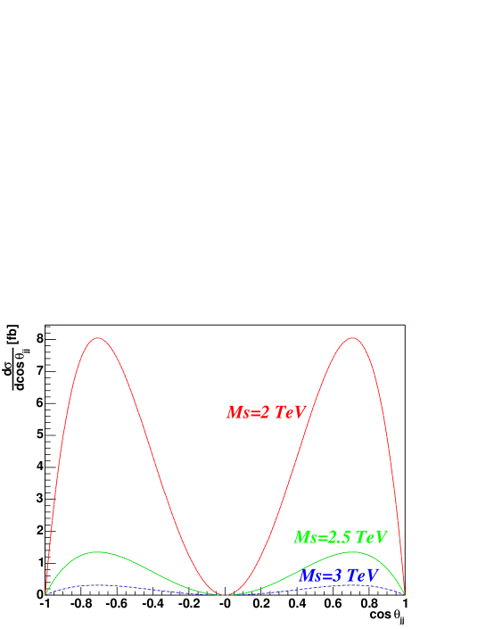
Figure 1: Angular dependence of the cross section $\frac{d\sigma(e^{+}e^{-}\rightarrow HH)}{d\cos\theta}$ [fb] (Eq. 8) as a function of the scattering angle ($\cos\theta$) for $M_{S}=2$, $2.5$, and 3 TeV, respectively, from top to bottom.

There are peaks in forward and backward regions. Notice also that the differential cross section vanishes at three points: $\cos\theta=0$ and $\pm 1$. This can be qualitatively understood in the following manner. Since the initial state consists of two spin-1/2 particles, the spin sum can not exceed 1. There must hence be some finite orbital angular momentum in the initial $e^{+}e^{-}$ system to make up the spin 2 of the intermediate KK gravitons. The orbital angular momentum is, however, perpendicular to the momentum, which means that the intermediate KK gravitons must have a spin component perpendicular to the beam axis. This component, however, has to be averaged to zero because of the rotational symmetry about the beam axis. On the other hand, since the structure of the energy momentum tensor of the initial state is chirality conserving, the initial-state spin sum and hence the spin of the KK gravitons must have a component of $\pm 1$ along the beam axis. Since the final-state Higgs bosons are spinless, this angular momentum of the KK gravitons has to be conserved by their orbital angular momentum. This implies that the final-state Higgs pair is in the $Y_{l}^{m}=Y_{2}^{\pm 1}$ state with the beam axis taken as its quantization axis. Eq. (7) indicates that this is indeed the case. Since $Y_{2}^{\pm 1}$ is odd in terms of $\cos\theta$, the cross section has to vanish at $\cos\theta=0$. Similarly the vanishment of the differential cross section at $\cos\theta=\pm 1$ can be interpreted as a consequence of the finite spin component in the beam direction: at $\cos\theta=\pm 1$ this component must vanish since the final-state orbital angular momentum is perpendicular to the beam axis.

3 Monte Carlo Simulation

3.1 Signal and Background Samples

A Monte Carlo event generator has been written for the Higgs pair production, using the above cross section formula. The generator generates 4-momenta of the final-state Higgs bosons, taking into account the initial state radiation and beamstrahlung and pass them to a hadronizer module of JLC Study Framework (JSF)[11, 13]. This hadronizer is based on Pythia 6[12], decays the final-state Higgs bosons into lighter partons, and makes them parton-shower and fragment, if necessary. The final-state jets of particles are then passed to the JSF’s quick detector simulator module to emulate the JLC detector response as described in [13]. The charged particle tracks and calorimeter clusters are then combined to measure energy flows from the individual jets and then used to reconstruct the final-state Higgs bosons as described below.

The signature of the signal process is the production of two pairs of $b$-jets whose mass is close to the mass of the Higgs. Other Standard Model processes producing two pairs of jets that mimic the signal will be our main backgrounds. The potential background processes thus include $e^{+}e^{-}\to W^{+}W^{-}$, $ZZ$, $ZH$ and $b\bar{b}b\bar{b}$. We used the physsim package [13, 14] and GRC4F[15] to generate these background events. The package works under JSF and uses full helicity amplitudes so that the angular correlations of the final state partons can be properly taken into account.

In what follows, we assume a linear collider of $\sqrt{s}=1$ TeV and study feasibility of measuring the angular distribution for the Higgs pair production process for $M_{S}=2~{}\mbox{TeV}$ and $m_{H}=120~{}\mbox{GeV}$.

3.2 Event Selection

Candidate events for the $e^{+}e^{-}\to HH$ process were selected among the signal and the background samples by applying the following set of selection criteria. The candidates had to have at least 25 tracks with an energy of at least 100 MeV each, a visible energy of at least 600 GeV, and a transverse momentum of less than 50 GeV. A jet finding algorithm (JADE type) was used to count the number of jets in the events and those with less than 4 jets at $y_{\mbox{cut}}=0.004$ were rejected. When there were more than 4 jets in an event, they were rearranged to form only 4 jets. Jets were then pair-combined to form all the possible Higgs candidates. Only events for which it was possible to form simultaneously 2 pairs whose invariant mass was less than 16 GeV away from the Higgs mass were kept. Figure 2 shows the distribution of the dijets invariant mass before the rejection of the candidates more than 16 GeV away from the higgs mass.

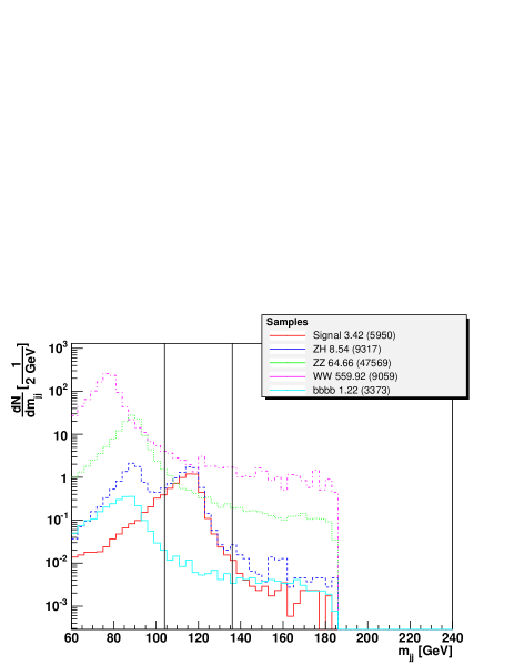
Figure 2: Distribution of the invariant masses of the dijets used as higgs candidates in 1 dimension (left) and in 2 dimensions (right). Only those which are less than 16 GeV away from the Higgs mass will be kept as Higgs candidates (the range kept is within the two vertical lines on the left plot and inside the boxes on the right plot). The numbers in this figure correspond to an integrated luminosity of 1 fb^-1 and the numbers in parentheses correspond to the number of Monte Carlo events.

To further improve the purity of the selection a $b$-tagging algorithm was used to require at least one of the jets of each Higgs candidate to be $b$-tagged.

Selection criteria	Signal	ZZ	ZH	WW	bbbb
No cut	5.772 (10000)	206.666 (150000)	18.395 (20000)	3833.3 (60000)	3.779 (10000)
$N_{\mbox{tracks}}>25$	5.674 (9831)	164.330 (119272)	18.202 (19790)	2427.1 (37990)	3.702 (9796)
$E_{\mbox{vis}}>600$ GeV	5.471 (9479)	90.856 (65944)	11.287 (12272)	1203.8 (18842)	2.310 (6111)
$P_{t}\leq 50$ GeV	3.662 (6345)	79.912 (58001)	8.9160 (9694)	939.61 (14707)	1.946 (5149)
$N_{\mbox{jets}}\geq 4$ at $y_{\mbox{cut}}=0.004$	3.481 (6031)	69.682 (50576)	8.6308 (9384)	644.89 (10094)	1.586 (4197)
$|m_{jj}-m_{H}|\leq 16$ GeV	2.234 (3870)	0.136 (99)	0.174 (190)	0.319 (5)	2.268 $\times 10^{-3}$ (6)
$b$-tagging	1.313 (2275)	0.006 (4)	0.038 (41)	0.0 (0)	3.78 $\times 10^{-4}$ (1)

Table 1: Cut statistics for the signal ($M_{S}=2$ TeV) and background event samples with $M_{S}=2$ TeV and $M_{h}=120$ GeV. The floating point numbers correspond to the numbers of remaining events per 1 fb^-1, while the numbers in parentheses represent the actual numbers of Monte Carlo events surviving the cuts. The cross sections include the effects of both initial state radiation and beamstrahlung.

Selection criteria	Signal	ZZ	ZH	WW
No cut	5.055 (10000)	206.666 (150000)	16.270 (20000)	3833.330 (60000)
$N_{\mbox{tracks}}>25$	4.975 (9841)	164.330 (119272)	16.185 (19895)	2427.137 (37990)
$E_{\mbox{vis}}>600$ GeV	4.841 (9577)	90.856 (65944)	10.798 (13273)	1203.800 (18842)
$P_{t}\leq 50$ GeV	3.235 (6400)	79.912 (58001)	8.555 (10516)	939.613 (14707)
$N_{\mbox{jets}}\geq 4$ at $y_{\mbox{cut}}=0.004$	3.123 (6177)	69.682 (50576)	8.308 (10212)	644.894 (10094)
$|m_{jj}-m_{H}|\leq 32$ GeV	2.506 (4958)	0.343 (249)	0.106 (130)	2.939 (46)
$b$-tagging	1.276 (2524)	0.063 (46)	0.030 (37)	0.000 (0)

Table 2: Cut statistics for the signal ($M_{S}=2$ TeV) and background event samples with $M_{S}=2$ TeV and $M_{h}=160$ GeV. The floating point numbers correspond to the numbers of remaining events per 1 fb^-1, while the numbers in parentheses represent the actual numbers of Monte Carlo events surviving the cuts. The cross sections include the effects of both initial state radiation and beamstrahlung.

Selection criteria	Signal	ZZ	ZH	WW
No cut	4.219 (10000)	206.666 (150000)	0.101 (20000)	3833.330 (60000)
$N_{\mbox{tracks}}>25$	4.151 (9838)	164.330 (119272)	0.100 (19758)	2427.137 (37990)
$E_{\mbox{vis}}>600$ GeV	4.052 (9603)	90.856 (65944)	0.061 (12141)	1203.793 (18842)
$P_{t}\leq 50$ GeV	2.745 (6507)	79.912 (58001)	0.048 (9613)	939.613 (14707)
$N_{\mbox{jets}}\geq 4$ at $y_{\mbox{cut}}=0.004$	2.678 (6346)	69.682 (50576)	0.047 (9325)	644.894 (10094)
$|m_{jj}-m_{H}|\leq 32$ GeV	1.909 (4524)	0.700 (508)	4.29$\times 10^{-4}$ (85)	8.242 (129)
$b$-tagging	0.842 (1995)	0.088 (64)	2.17$\times 10^{-4}$ (43)	0.127778 (2)

Table 3: Cut statistics for the signal ($M_{S}=2$ TeV) and background event samples with $M_{S}=2$ TeV and $M_{h}=200$ GeV. The floating point numbers correspond to the numbers of remaining events per 1 fb^-1, while the numbers in parentheses represent the actual numbers of Monte Carlo events surviving the cuts. The cross sections include the effects of both initial state radiation and beamstrahlung.

Selection criteria	Signal ($M_{S}=2$ TeV)	Signal ($M_{S}=2.5$ TeV)	Signal ($M_{S}=3$ TeV)
No cut	5.772 (10000)	0.968 (10000)	0.045 (2012)
$N_{\mbox{tracks}}>25$	5.674 (9831)	0.952 (9829)	0.221 (9829)
$E_{\mbox{vis}}>600$ GeV	5.471 (9479)	0.918 (9480)	0.213 (9480)
$P_{t}\leq 50$ GeV	3.662 (6345)	0.615 (6351)	0.143 (6351)
$N_{\mbox{jets}}\geq 4$ at $y_{\mbox{cut}}=0.004$	3.481 (6031)	0.584 (6028)	0.136 (6028)
$|m_{jj}-m_{H}|\leq 16$ GeV	2.234 (3870)	0.374 (3861)	0.087 (3861)
$b$-tagging	1.313 (2275)	0.219 (2264)	0.051 (2264)

Table 4: Cut statistics for the signal for three differnt values of $M_{S}$: $M_{S}=2$ TeV , $M_{S}=2.5$ TeV and $M_{S}=3$ TeV with $M_{h}=120$ GeV. The floating point numbers correspond to the numbers of remaining events per 1 fb^-1, while the numbers in parentheses represent the actual numbers of Monte Carlo events surviving the cuts. The cross sections include the effects of both initial state radiation and beamstrahlung. These number of event scale like $\frac{1}{M_{S}^{8}}$, as expected from Eq.(8).

Tables 1, 2 and 3 summarizes the number of surviving events per 1 fb^-1 at each step of the selection cuts for both the signal and background event samples for different values of the Higgs mass ($M_{h}=120$ GeV, $M_{h}=160$ GeV and $M_{h}=200$ GeV). The table 4 confirms that the signal’s differential cross section scales like $\frac{1}{M_{S}^{8}}$, as calculated in Eq.(8). These tables show that the above selection criteria reject almost all the backgrounds, while keeping a reasonable detection efficiency around 20% for the signal process. For the sample set of parameters, $M_{S}=2~{}\mbox{TeV}$ and $m_{H}=120~{}\mbox{GeV}$, this corresponds to about 700 events at $\sqrt{s}=1$ TeV for an integrated luminosity of 500 fb^-1. For the processes $e^{+}e^{-}\rightarrow ZZ$ and $e^{+}e^{-}\rightarrow W^{+}W^{-}$ only the Standard Model contribution has been considered. Since these processes could also be mediated by virtual KK gravitons and hence be enhanced, the $e^{+}e^{-}\to ZZ$ process would have become the dominant background. Even so, the number of events surviving the selection criteria would remain at least one order of magnitude lower than our signal. On the other hand, the $e^{+}e^{-}\to ZH$ background would stay the same, since there would be no virtual KK graviton contribution.

3.3 Reconstruction of Angular Distribution

Using the selected Higgs pair candidates, we can now look at the angular distribution of the reconstructed Higgs pairs. Figure 3 shows a typical distribution of the reconstructed $\cos\theta$ of the selected events compared to the shape expected from Eq. 8 (green dotted curve). The discrepancy near $\cos\theta_{\mbox{jj}}=\pm 1$ comes from the limited acceptance of the detector near the beam pipe.

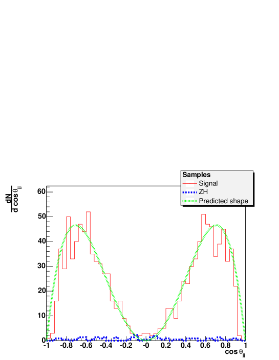
Figure 3: Distribution of the $\cos\theta_{\mbox{jet}}$ of the signal events (in red) and the ZH background (in blue) after application of the selection criteria. The numbers in this figure correspond to an integrated luminosity of 500 fb^-1.

The reconstructed $\cos\theta$ distribution clearly exhibits the characteristic spin-2 behavior, demonstrating the possibility of the test of KK graviton spin exchanged in the $s$-channel.

4 Summary and Conclusions

We have derived the cross section formula for the process $e^{+}e^{-}\to HH$ via $s$-channel KK graviton exchange. We have found that the cross section at $\sqrt{s}=1$ TeV is of the same order of magnitude as that of the associated higgs production cross section, $e^{+}e^{-}\rightarrow ZH$ in the standard model, for a sample parameter set, $M_{S}=2~{}\mbox{TeV}$ and $m_{H}=120~{}\mbox{GeV}$.

It should be stressed that the differential cross section gives a characteristic behavior reflecting the spin 2 nature of the intermediate KK gravitons. The cross section formula was then used to carry out Monte Carlo simulations to test the feasibility of measuring this angular distribution. We have shown that, for our sample set of parameters, we can obtain about 700 Higgs pair events at $\sqrt{s}=1$ TeV, given an integrated luminosity of 500 fb^-1, with essentially no Standard Model backgrounds. Even if $M_{S}$ is higher the $2$ TeV but remains below 2500 GeV, we will be able to accumulate more than 100 events at $\sqrt{s}=1$TeV and observe the characteristic angular distribution. Conversely, if $M_{S}=4$TeV, we would need to accumulate 500 $fb^{-1}$ at $\sqrt{s}=3.4$ TeV or higher to be able to accumulate 100 Higgs pair events.

Using this very clean sample, we have then demonstrated that we can indeed measure the characteristic angular distribution of the Higgs pair production via the KK graviton exchange.

Finally, as mentionned in section 4, the processes $e^{+}e^{-}\rightarrow ZZ$ and $e^{+}e^{-}\rightarrow W^{+}W^{-}$ can also be mediated by virtual KK gravitons. This has not been taken into account in our simulations but our estimations shows that in the worse case the $ZZ$ cross section would be enhanced 4 times and the $WW$ cross section 40% higher, thus the background coming from these processes would remain very small.

The processes $e^{+}e^{-}\rightarrow ZZ$ and $e^{+}e^{-}\rightarrow W^{+}W^{-}$ mediated by virtual KK gravitons are certainly worth investigating for the linear collider studies of extra dimension scenarios [16].

Acknowledgments

The authors would like to thank all the members of the new physics subgroup of the LC physics study group in Japan. Among them Shinji Komine deserves special mention for his contribution in the early stage of this work. One of the authors (ND) would also like to thank JSPS for funding his stay in Japan under contract P02794. This work is partially supported by JSPS-CAS Scientific Cooperation Program under the Core University System and by Japan-Europe (UK) Research Cooperative Program of JSPS.

References

- [1] N. Arkani-Hamed, S. Dimopoulos and G. R. Dvali, Phys. Lett. B 429, 263 (1998) [arXiv:hep-ph/9803315]; I. Antoniadis, N. Arkani-Hamed, S. Dimopoulos and G. R. Dvali, Phys. Lett. B 436, 257 (1998) [arXiv:hep-ph/9804398].
- [2] C. D. Hoyle, U. Schmidt, B. R. Heckel, E. G. Adelberger, J. H. Gundlach, D. J. Kapner and H. E. Swanson, Phys. Rev. Lett. 86, 1418 (2001) [arXiv:hep-ph/0011014].
- [3] For a review, see, for example, K. Cheung, arXiv:hep-ph/0305003, and references therein.
- [4] T. G. Rizzo, Phys. Rev. D 60 (1999) 075001 [arXiv:hep-ph/9903475].
- [5] C. S. Kim, K. Y. Lee and J. Song, Phys. Rev. D 64, 015009 (2001) [arXiv:hep-ph/0009231].
- [6] X. G. He, Phys. Rev. D 60, 115017 (1999) [arXiv:hep-ph/9905295].
- [7] G. F. Giudice, R. Rattazzi and J. D. Wells, Nucl. Phys. B 544, 3 (1999) [arXiv:hep-ph/9811291];
- [8] T. Han, J. D. Lykken and R. J. Zhang, Phys. Rev. D 59, 105006 (1999) [arXiv:hep-ph/9811350].
- [9] M. Bando, T. Kugo, T. Noguchi and K. Yoshioka, Phys. Rev. Lett. 83, 3601 (1999) [arXiv:hep-ph/9906549].
- [10] J. Hisano and N. Okada, Phys. Rev. D 61, 106003 (2000) [arXiv:hep-ph/9909555].
- [11] JSF Quick Simulator, http://www-jlc.kek.jp/subg/offl/jsf/ .
- [12] T. Sjöstrand, L. Lönnblad, S. Mrenna, P. Skands, [arXiv:hep-ph/0108264].
- [13] ACFA LC working group, KEK Report, 01-11 (2001), hep-ph/0109166.
- [14] http://www-jlc.kek.jp/subg/offl/physsim/ .
- [15] J. Fujimoto et al., Comput. Phys. Commun. 100 (1997) 128 [arXiv:hep-ph/9605312].
- [16] N. Delerue, K. Fujii and N.Okada, in progress.