$B$ meson decays to $\eta^{(\prime)}K^{*}$, $\eta^{(\prime)}\rho$, $\eta^{(\prime)}\pi^{0}$, $\omega\pi^{0}$, and $\phi\pi^{0}$

Abstract

We present measurements of the branching fractions and charge asymmetries (where appropriate) of two-body $B$ decays to $\eta^{(\prime)}K^{*}$, $\eta^{(\prime)}\rho$, $\eta^{(\prime)}\pi^{0}$, $\omega\pi^{0}$, and $\phi\pi^{0}$. The data were recorded with the BABAR detector at PEP-II and correspond to $89\times 10^{6}$ $B\kern 1.79993pt\overline{\kern-1.79993ptB}{}$ pairs produced in $e^{+}e^{-}$ annihilation through the $\mathchar 28935\relax(4S)$ resonance. We find significant signals for two decay modes and measure the branching fractions ${\cal B}(B^{+}\rightarrow\eta K^{*+})=(25.6\pm 4.0\pm 2.4\,)\times 10^{-6}$ and ${\cal B}(B^{0}\rightarrow\eta K^{*0})=(18.6\pm 2.3\pm 1.2)\times 10^{-6}$, where the first error is statistical and the second systematic. We also find evidence with significance $3.5\sigma$ for a third decay mode and measure ${\cal B}(B^{+}\rightarrow\eta\rho^{+})=(9.2\pm 3.4\pm 1.0)\times 10^{-6}$. For other channels, we set $90\%$ C.L. upper limits of ${\cal B}(B^{0}\rightarrow\eta\rho^{0})<1.5\times 10^{-6}$, ${\cal B}(B^{+}\rightarrow\eta^{\prime}K^{*+})<14\times 10^{-6}$, ${\cal B}(B^{0}\rightarrow\eta^{\prime}K^{*0})<7.6\times 10^{-6}$, ${\cal B}(B^{+}\rightarrow\eta^{\prime}\rho^{+})<22\times 10^{-6}$, ${\cal B}(B^{0}\rightarrow\eta^{\prime}\rho^{0})<4.3\times 10^{-6}$, ${\cal B}(B^{0}\rightarrow\eta\pi^{0})<2.5\times 10^{-6}$, ${\cal B}(B^{0}\rightarrow\eta^{\prime}\pi^{0})<3.7\times 10^{-6}$, ${\cal B}(B^{0}\rightarrow\omega\pi^{0})<1.2\times 10^{-6}$, and ${\cal B}(B^{0}\rightarrow\phi\pi^{0})<1.0\times 10^{-6}$. For self-flavor-tagging modes with significant signals, the time-integrated charge asymmetries are ${\cal A}_{ch}(\eta K^{*+})=+0.13\pm 0.14\pm 0.02$ and ${\cal A}_{ch}(\eta K^{*0})=+0.02\pm 0.11\pm 0.02$.

I Introduction

We report the results of searches for charged or neutral $B$-meson decays to the charmless final states CC $\eta K^{*}$, $\eta^{\prime}K^{*}$, $\eta\rho$, $\eta^{\prime}\rho$, $\eta\pi^{0}$, $\eta^{\prime}\pi^{0}$, $\omega\pi^{0}$, and $\phi\pi^{0}$. For decays that are self-tagging with respect to the $b$ or $\overline{b}$ flavor, we also measure the direct $C\!P$-violating time-integrated charge asymmetry,

$${\cal A}_{ch}=\frac{\Gamma^{-}-\Gamma^{+}}{\Gamma^{-}+\Gamma^{+}}~{}.$$ (1)

The superscript on $\Gamma$ corresponds to the sign of the $B^{\pm}$ meson or the sign of the charged kaon for $B^{0}$ decays. Throughout this paper, we use $\eta^{(\prime)}$ to indicate either $\eta$ or $\eta^{\prime}$.

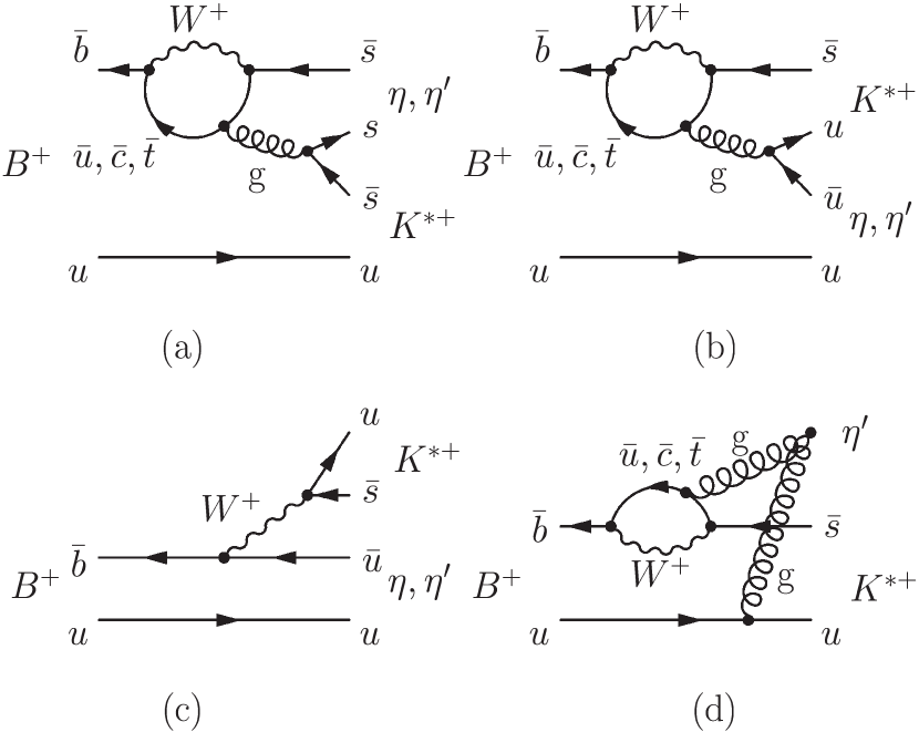
Figure 1: Feynman diagrams for the decays $Bp\rightarrow(\eta,\eta^{\prime})K^{*+}$. The corresponding neutral decays are similar except that the spectator quark becomes a $d$, the gluon in (b) makes $d\bar{d}$, and the tree diagram in (c) has an internal $W$.

Interest in $B$ decays to $\eta$ or $\eta^{\prime}$ final states intensified in 1997 with the CLEO observation of the decay $B\rightarrow\eta^{\prime}K$ CLEOetapobs . It had been pointed out by Lipkin six years earlier Lipkin that interference between two penguin diagrams (see Figs. 1a and 1b) and the known $\eta/\eta^{\prime}$ mixing angle conspire to greatly enhance $B\rightarrow\eta^{\prime}K$ and suppress $B\rightarrow\eta K$. Because the vector $K^{*}$ has the opposite parity from the kaon, the situation is reversed for the $B\rightarrow\eta^{\prime}K^{*}$ and $B\rightarrow\eta K^{*}$ decays. The general features of this picture have already been verified by previous measurements and limits. However, the details and possible contribution of the flavor-singlet diagram (Fig. 1d) can only be tested with the measurement of the branching fractions of all four $(\eta,\eta^{\prime})(K,K^{*})$ decays; the branching fraction of the $B\rightarrow\eta^{\prime}K^{*}$ decay is expected to be particularly sensitive to a flavor-singlet component chiang ; beneke . The tree diagram (Fig. 1c) is suppressed by the parameter $\lambda$ of the Cabibbo-Kobayashi-Maskawa (CKM) mixing matrix.

By contrast, for the $B\rightarrow\eta^{(\prime)}\rho^{+}$ decays, the penguin diagrams (Figs. 2c and 2d) are CKM- suppressed. Since the internal tree diagram (Fig. 2b) is color-suppressed, the decay is dominated by the (external) tree diagram of Fig. 2a.

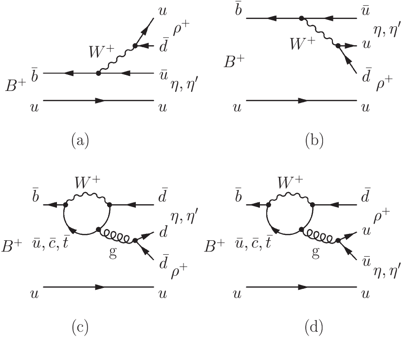
Figure 2: Feynman diagrams for the decays $B^{+}\rightarrow\eta\rho^{+}$ and $B^{+}\rightarrow\eta^{\prime}\rho^{+}$.

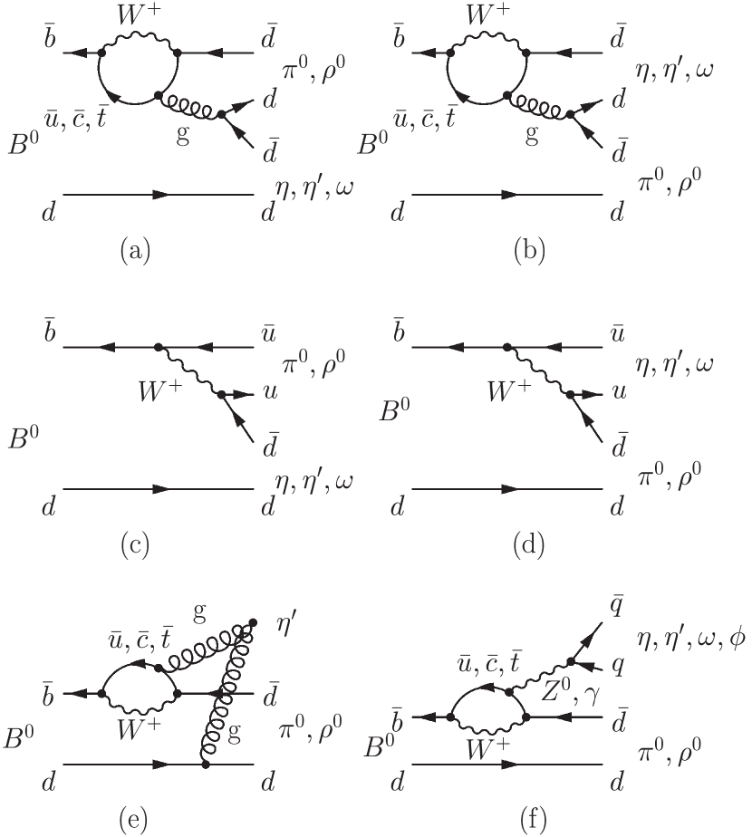
Figure 3: Feynman diagrams for the $B^{0}$ decays.

The $B^{0}$ decays are different because there are no external tree diagrams analogous to Fig. 2a. In Figs. 3a and 3b we show the penguin diagrams and in Figs. 3c and 3d the color-suppressed tree diagrams for the $B^{0}\rightarrow\eta^{(\prime)}\rho^{0}$, $B^{0}\rightarrow\eta^{(\prime)}\pi^{0}$, and $B^{0}\rightarrow\omega\pi^{0}$  decays. The color-suppressed diagrams cancel for the $\eta$ and $\eta^{\prime}$  decays and are expected to be largely suppressed for the pseudoscalar-vector ($PV$) $B^{0}\rightarrow\omega\pi^{0}$ decay. The singlet penguin diagram (Fig. 3e) may be significant only for the decays with an $\eta^{\prime}$ in the final state, and the electroweak penguin (Fig. 3f) is the only contribution for the $B^{0}\rightarrow\phi\pi^{0}$ decay (and negligible for the other decay modes). Branching fractions for all these decays are generally expected to be in the range (0.1–10)$\times 10^{-6}$ kramer ; grabbag ; yang ; CGR , with the $B^{+}\rightarrow\eta^{(\prime)}\rho^{+}$ decays at the high end of this range and the $B^{0}$ decays at the low end (and $B^{0}\rightarrow\phi\pi^{0}$ perhaps somewhat below this range).

The charge asymmetry ${\cal A}_{ch}$ for most of these decays is expected to be ${~{}\raise 1.49994pt\hbox{$<$}\kern-8.50006pt\lower 3.50006pt\hbox{$\sim$}~{}}10$% kramer ; AKLasym . However, for $B\rightarrow\eta^{\prime}K^{*}$ the penguin and tree amplitudes are expected to be of similar magnitude, which allows charge asymmetries which could be in the $(20-40)$% range beneke ; yang ; CGR ; dighe . Information on charge asymmetries and branching fractions from this full collection of $B$ decays can serve to constrain the relationship between the various underlying amplitudes.

The results described in this paper complete the measurement of all four $(\eta,\eta^{\prime})(K,K^{*})$ final states, as well as those with $(\eta,\eta^{\prime})(\pi,\rho)$, with a BABAR dataset of 89 million $B\kern 1.79993pt\overline{\kern-1.79993ptB}{}$ decays. Current knowledge of the decays discussed here comes from published measurements from CLEO CLEOetapr ; CLEOomega ; CLEOphipiz and BABAR BABARetapOmega . Results for the final states $(\eta,\eta^{\prime})(K,\pi)$ on this dataset have been presented elsewhere etaprPRL ; etaomegaPRL . These data represent an order of magnitude increase in the $B$ meson sample size over the only previous complete study.

All results are based on extended maximum likelihood (ML) fits as described in Section V. In each analysis, loose criteria are used to select events likely to contain the desired signal $B$ decay. A fit to kinematic and topological discriminating variables is used to differentiate between signal and background events and to determine signal event yields and time-integrated rate asymmetries. In all of the decays analyzed, the background is dominated by random particle combinations in continuum ($e^{+}e^{-}\rightarrow q{\bar{q}}$, $q=u,d,s,c$ ) events. Some decay modes also suffer backgrounds from other charmless $B$ decays with topologies similar to that of the signal. In such cases, these backgrounds are accounted for explicitly in the fit as discussed in Sec. IV.3. Signal event yields are converted into branching fractions via selection efficiencies determined from Monte Carlo simulations of the signal as well as auxiliary studies of the data. The complete analysis is carried out without regard to whether there are observed signals. This “blind” procedure is used to avoid bias in the results.

II Detector and Data

The results presented in this paper are based on data collected with the BABAR detector BABARNIM at the PEP-II asymmetric-energy $e^{+}e^{-}$ collider pep located at the Stanford Linear Accelerator Center. The results in this paper correspond to an accumulated integrated luminosity of approximately 82 $\mbox{\,fb}^{-1}$, corresponding to 89 million $B\kern 1.79993pt\overline{\kern-1.79993ptB}{}$ pairs, recorded at the $\mathchar 28935\relax(4S)$ resonance (“on-peak”, center-of-mass energy $\sqrt{s}=10.58\ \mathrm{\,Ge\kern-1.00006ptV}$). An additional 9.6 $\mbox{\,fb}^{-1}$ were recorded about 40 MeV below this energy (“off-peak”) for the study of continuum backgrounds in which a light or charm quark pair is produced.

The asymmetric beam configuration in the laboratory frame provides a boost of $\beta\gamma=0.56$ to the $\mathchar 28935\relax(4S)$. This results in a charged-particle laboratory momentum spectrum from $B$ decays with an endpoint near 4 $\mathrm{\,Ge\kern-1.00006ptV}$. Charged particles are detected and their momenta measured by the combination of a silicon vertex tracker (SVT), consisting of five layers of double-sided detectors, and a 40-layer central drift chamber, both operating in the 1.5-T magnetic field of a solenoid. The transverse momentum resolution for the combined tracking system is $\sigma_{p_{T}}/p_{T}=0.0013p_{T}\oplus 0.0045$, where the sum is in quadrature and $p_{T}$ is measured in $\mathrm{\,Ge\kern-1.00006ptV}$. For charged particles within the detector acceptance resulting from the $B$ decays studied in this paper, the average detection efficiency is in excess of 96% per particle. Photons are detected and their energies measured by a CsI(Tl) electromagnetic calorimeter (EMC). The photon energy resolution is $\sigma_{E}/E=\left\{2.3/E(\mathrm{\,Ge\kern-1.00006ptV})^{1/4}\oplus 1.9\right\}\%$, and the angular resolution from the interaction point is $\sigma_{\theta}=3.9^{\rm o}/\sqrt{E(\mathrm{\,Ge\kern-1.00006ptV})}$. The photon energy scale is determined using symmetric $\pi^{0}\rightarrow\gamma\gamma$ decays. The measured $\pi^{0}$ mass resolution for $\pi^{0}$’s with laboratory momentum in excess of 1 $\mathrm{\,Ge\kern-1.00006ptV}$ is approximately 8 MeV.

Charged-particle identification (PID) is provided by the average energy loss ($\mathrm{d}E/\mathrm{d}x$) in the tracking devices and by an internally reflecting ring-imaging Cherenkov detector (DIRC) covering the central region. The $\mathrm{d}E/\mathrm{d}x$ resolution from the drift chamber is typically about $7.5\%$ for pions. The Cherenkov angle resolution of the DIRC is measured to be 2.4 mrad, which provides a nearly $3\sigma$ separation between charged kaons and pions at a momentum of $3~{}\mathrm{\,Ge\kern-1.00006ptV}$. Additional information that we use to identify and reject electrons and muons is provided by the EMC and the detectors of the solenoid flux return (IFR).

III Candidate Reconstruction and $B$ Meson Selection

We reconstruct $B$ mesons in the final states $\eta^{(\prime)}$$K^{*+}$, $\eta^{(\prime)}$$K^{*0}$, $\eta^{(\prime)}$$\rho^{+}$, $\eta^{(\prime)}$$\rho^{0}$, $\eta^{(\prime)}$$\pi^{0}$, $\omega\pi^{0}$, and $\phi\pi^{0}$. Monte Carlo (MC) simulations geant  of the signal decay modes and of continuum and $B\kern 1.79993pt\overline{\kern-1.79993ptB}{}$ backgrounds, and data control samples of similar modes, are used to establish the event selection criteria. The selection is designed to achieve high efficiency and retain sufficient sidebands in the discriminating variables to characterize the background for subsequent fitting. As the invariant mass distributions from the primary resonances ($\eta^{(\prime)}$, $K^{*}$, $\rho$, ${\omega}$, and $\phi$) in the decay are included in the maximum likelihood fit, the selection criteria are generally loose. Additional states—$\pi^{0}$ or $\eta$ in $\eta^{\prime}$ decays, and $K^{0}_{\scriptscriptstyle S}$—are selected with the requirement that the invariant mass lie within 2-3$\sigma$ of the known mass.

III.1 Charged track selection

We require all charged-particle tracks (except for those from the $K^{0}_{\scriptscriptstyle S}\rightarrow\pi^{+}\pi^{-}$ decay) used in reconstructing the $B$ candidate to include at least twelve point measurements in the drift chamber, lie in the polar angle range $0.41<\theta_{lab}<2.54$ rad, and originate from within 1.5 cm in the $x-y$ plane and 10 cm in the $z$ direction from the nominal beam spot. We require the tracks to have a transverse momentum $p_{T}$ of at least 100 MeV.

We also place requirements on particle identification criteria. We veto leptons from our samples by demanding that tracks have DIRC, EMC and IFR signatures that are inconsistent with either electrons or muons. The remaining tracks are assigned as either charged pion or kaon candidates. This assignment is based on a likelihood selection developed from $\mathrm{d}E/\mathrm{d}x$ and Cherenkov angle information from the tracking detectors and DIRC, respectively. For the typical laboratory momentum spectrum of the signal kaons, this selection has an efficiency of about 85% and a pion misidentification rate of less than 2%, as determined from control samples of $D^{*}\rightarrow D^{0}\pi$, $D^{0}\rightarrow K\pi$ events. The detailed performance of the kaon selection has been characterized as a function of laboratory momentum and can be seen in Fig. 4.

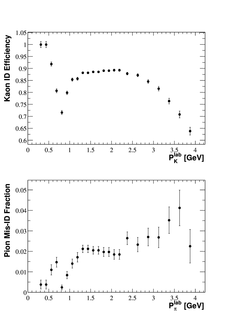
Figure 4: Identification (ID) efficiency of the charged kaon selection as a function of the kaon laboratory momentum $P_{K}^{\rm lab}$ (top), and fraction of charged pions misidentified (mis-ID) as kaons as a function of the pion laboratory momentum $P_{\pi}^{\rm lab}$ (bottom). The error bars represent statistical uncertainties in the control sample of kaons and pions from $D^{*}\rightarrow D^{0}\pi$, $D^{0}\rightarrow K\pi$ decays.

III.2 $\eta^{(\prime)},~{}{\omega},~{}\rm{and}~{}\phi$ selection

We reconstruct the $\eta$ in two final states: $\eta\rightarrow\gamma\gamma$ ($\eta_{\gamma\gamma}$) and $\eta\rightarrow\pi^{+}\pi^{-}\pi^{0}$ ($\eta_{3\pi}$). For the $\eta^{\prime}$, we reconstruct two final states: $\eta^{\prime}\rightarrow\rho^{0}\gamma$ ($\eta^{\prime}_{\rho\gamma}$) and $\eta^{\prime}\rightarrow\eta\pi^{+}\pi^{-}$ ($\eta^{\prime}_{\eta\pi\pi}$), with $\eta\rightarrow\gamma\gamma$ (except in the $\eta^{\prime}_{\eta(3\pi)\pi\pi}K^{*0}$ mode, where we also include $\eta\rightarrow\pi^{+}\pi^{-}\pi^{0}$). In the $B^{0}\rightarrow\omega\pi^{0}$ channel, we reconstruct $\omega\rightarrow\pi^{+}\pi^{-}\pi^{0}$; for $B^{0}\rightarrow\phi\pi^{0}$ we reconstruct $\phi\rightarrow K^{+}K^{-}$. We place the following requirements on the invariant masses of the resonance candidates (in MeV): $520<m_{\eta_{3\pi}}<570$, $490<m_{\eta_{\gamma\gamma}}<600$, $910<m_{\eta^{\prime}}<1000$ for $\eta^{\prime}_{\rho\gamma}$ and $\eta^{\prime}_{\eta\pi\pi}$, $735<m_{\omega}<835$, and $990<m_{\phi}<1050$. These ranges can be seen graphically in Fig. 8 in Sec. VI.2. The mass requirements for these resonances are loose to keep appropriate sidebands for fitting; the resonance shapes used for fitting are discussed in Sec. VI.

For $\eta\rightarrow\gamma\gamma$ candidates we require $|{\cal H}_{\eta}|$ to be less than 0.86, where ${\cal H}_{\eta}$ is the cosine of the $\eta$ decay angle. The decay angle is defined, in the $\eta$ rest frame, as the angle between one of the photons and the direction of the boost needed to get to this frame from the $B$ center-of-mass (CM) frame. This requirement removes very asymmetric decays of the $\eta$, where one photon carries most of the particle’s energy. It is effective against high-energy background photons from $B\rightarrow K^{*}\gamma$ that combine with a random low-energy photon to form an invariant mass in the range chosen for the $\eta\rightarrow\gamma\gamma$ decay. For the $\eta^{\prime}_{\eta\pi\pi}\rho^{+}$ channel, the $\eta\rightarrow\gamma\gamma$ mass range is tightened to $510<m_{\gamma\gamma}<580$ $\mathrm{\,Me\kern-1.00006ptV}$ to reduce the continuum background in the sample.

III.3 Photon and $\pi^{0}$ selection

Photons are reconstructed from energy depositions in the electromagnetic calorimeter which are not associated with a charged track. We require that all photon candidates have an energy greater than 30 $\mathrm{\,Me\kern-1.00006ptV}$ except for the modes $\eta^{(\prime)}\pi^{0}$, $\omega\pi^{0}$, and $\phi\pi^{0}$, where there is significant combinatorial background arising from low-energy photons. For these modes, we tighten the photon-energy requirement to 50 $\mathrm{\,Me\kern-1.00006ptV}$ for all photons. For $\eta\rightarrow\gamma\gamma$, we require each photon energy to be greater than 100 $\mathrm{\,Me\kern-1.00006ptV}$, and for the $\eta^{\prime}\rightarrow\rho^{0}\gamma$ modes, we require the photon from the $\eta^{\prime}$ decay to exceed 200 $\mathrm{\,Me\kern-1.00006ptV}$.

We select neutral-pion candidates from two photon clusters with the requirement that the $\gamma\gamma$  invariant mass satisfy $120<m_{\pi^{0}}<150$ $\mathrm{\,Me\kern-1.00006ptV}$. The mass of a $\pi^{0}$  candidate meeting this criterion is then constrained to the nominal value PDG2002 and, when combined with other tracks or neutrals to form a $B$ candidate, to originate from the $B$ candidate vertex. This procedure improves the mass and energy resolution of the parent particle.

For the primary $\pi^{0}$ in $\eta^{(\prime)}\pi^{0}$ decays, photon candidates are required to be consistent with the expected lateral shower shape, and the magnitude of the cosine of the $\pi^{0}$  decay angle (defined as for the $\eta$) must be less than 0.95.

III.4 $K^{0}$ selection

For decay chains containing a $K^{0}$, we reconstruct only the $K^{0}_{\scriptscriptstyle S}\rightarrow\pi^{+}\pi^{-}$ decay. The invariant mass of the candidate $K^{0}_{\scriptscriptstyle S}$ is required to lie within the range $488<m_{\pi^{+}\pi^{-}}<508$ $\mathrm{\,Me\kern-1.00006ptV}$. We also perform a vertex-constrained fit to require that the two tracks originate from a common vertex, and require that the lifetime significance of the $K^{0}_{\scriptscriptstyle S}$ ($\tau/\sigma_{\tau}$) be $>3$, where $\sigma_{\tau}$ is the uncertainty in the lifetime determined from the vertex-constrained fit.

III.5 $K^{*}$ and $\rho$ selection

We reconstruct the $K^{*+}$ as either $K^{+}\pi^{0}$ ($K^{*+}_{K^{+}\pi^{0}}$) or $K^{0}_{\scriptscriptstyle S}\pi^{+}$ ($K^{*+}_{K^{0}\pi^{+}}$), and the $K^{*0}$ as $K^{+}\pi^{-}$ ($K^{*0}_{K^{+}\pi^{-}}$). The $\rho^{+}$ is reconstructed as $\pi^{+}\pi^{0}$ and the $\rho^{0}$ as $\pi^{+}\pi^{-}$. A vertex fit is performed when reconstructing the resonant $K^{*}$ or $\rho$ candidate. We require the invariant masses (in MeV) of the resonance candidates to be in the ranges: $755<m_{K\pi}<1035$, $470<m_{\pi^{+}\pi^{0}}<1070$, and $510<m_{\pi^{+}\pi^{-}}<1060$. The lower limit on the $\rho^{0}$ candidate invariant mass is chosen to reject background from $K^{0}_{\scriptscriptstyle S}$ decays.

For decay chains involving a charged $K^{*}$ or $\rho$, we define ${\cal H}$, the cosine of the angle between the pion and the negative of the $B$ momentum in the vector-meson rest frame. For $\rho^{+}$ decays, the direction is that of the $\pi^{0}$. For $\rho^{0}$ decays, we use only the magnitude of ${\cal H}$, which is independent of the choice of reference pion. For these decays with a $\pi^{0}$ in the final state, we require that ${\cal H}$ be greater than $-0.5$ to reject combinatorial background.

III.6 $B$ meson selection

A $B$-meson candidate is characterized kinematically by the energy-substituted mass $m_{\rm ES}$ and by the energy difference $\Delta E$, defined as

$$m_{\rm ES} = \sqrt{\left(\frac{{1\over 2}s+{\bf p}_{0}\cdot{\bf p}_{B}}{E_{0}}\right)^{2}-{\bf p}_{B}^{2}}\qquad\mbox{and}$$ (2)

$$\Delta E = \left(2q_{0}q_{B}-s\right)/2\sqrt{s}\ ,$$ (3)

where $q_{B}=(E_{B},{\bf p}_{B})$ and $q_{0}=(E_{0},{\bf p}_{0})$ are the four vectors of the $B$-candidate and the initial electron-positron system, respectively, and $s$ is the square of the invariant mass of the electron-positron system. When expressed in the $\mathchar 28935\relax(4S)$ frame, these quantities take the simpler but equivalent form

$$m_{\rm ES} = \sqrt{{1\over 4}s-{\bf p}_{B}^{*2}}\qquad\mbox{and}$$ (4)

$$\Delta E = E_{B}^{*}-{1\over 2}\sqrt{s}\ ,$$ (5)

where the asterisk denotes the value in the $\mathchar 28935\relax(4S)$ frame. The mode-dependent resolutions on these quantities for signal events are about $3\ \mathrm{\,Me\kern-1.00006ptV}$ for $m_{\rm ES}$, and 30–60 MeV for $\Delta E$.

We require $5.20\leq\mbox{$m_{\rm ES}$}\leq 5.29\ \mathrm{\,Ge\kern-1.00006ptV}$ and $|\Delta E|\leq 0.2$ $\mathrm{\,Ge\kern-1.00006ptV}$ for all but the $\eta^{(\prime)}\pi^{0}$, $\omega\pi^{0}$, and $\phi\pi^{0}$ modes, where we loosen the $\Delta E$ range to $|\Delta E|\leq 0.3$ $\mathrm{\,Ge\kern-1.00006ptV}$ to account for poorer detector resolution in these channels.

When multiple $B$ candidates from the same event pass the selection requirements, we choose a single candidate based on criteria described below. The average number of candidates per event depends on the mode; it is typically about 1.2 and is always less than 1.5. We find that 70–90% of the events have a single combination and about 90% of the rest have two combinations. In decays containing an $\eta$ and a $K^{*}$ or $\rho$, we select the candidate with the smallest $\chi^{2}$ formed from the $\eta$ and $K^{*}$ or $\rho$ masses. For decays containing $\eta^{\prime}\rightarrow\eta\pi^{+}\pi^{-}$, the $\chi^{2}$ is formed from the masses of the $\eta^{\prime}$ and $\eta$ candidates. For all other decays, we retain the candidate that has the mass of the primary resonance ($\eta^{(\prime)}$, ${\omega}$, or $\phi$) closest to the nominal value PDG2002 . We have checked that this choice introduces no significant yield bias, in part because, for the primary resonance mass, there is an adjustable peaking component included in the fit, which would account for any small distortion due to this selection.

IV Sources of Background and Suppression Techniques

Production of $B{\bar{B}}$ pairs accounts for a relatively small fraction of the $e^{+}e^{-}$ cross section even at the peak of the $\mathchar 28935\relax(4S)$ resonance. Upsilon production amounts to about 25% of the total hadronic cross section, while tau-pair production and other QED processes occur as well. We describe below several sources of background, and discuss techniques for distinguishing them from signal.

IV.1 QED and tau-pair backgrounds

Two-photon processes, Bhabha scattering, muon-pair production and tau pair production are characterized by low charged track multiplicities. Bhabha and muon-pair events are significantly prescaled at the trigger level. We further suppress these and other tau and QED processes via a minimum requirement on the event track multiplicity. We require the event to contain at least one track more than the topology of our final state, or three tracks, whichever is larger. We also place a requirement on the ratio of the second to the zeroth Fox–Wolfram moments FoxW , $R_{2}<0.98$, calculated with both charged tracks and neutral energy depositions. These selection criteria are more than 90% efficient when applied to signal. From MC simulations we have determined that the remaining background from these sources is negligible.

IV.2 QCD continuum backgrounds

The primary source of background to all charmless hadronic decays of the $B$ meson arises from continuum quark-antiquark production. The fact that these events are produced well above threshold provides the means by which they can be rejected, as the hadronization products are produced in a jet-like topology. In strong contrast, $B$ mesons resulting from $\mathchar 28935\relax(4S)$ decays are produced just above threshold. Thus the final-state particles in the signal are distributed approximately isotropically in the CM frame.

Several event-shape variables are designed to take advantage of this difference. We define the thrust axis for a collection of particles as the axis that maximizes the sum of the magnitudes of the longitudinal momenta with respect to the axis. The angle $\theta_{T}$ between the thrust axis of the $B$ candidate and that of the rest of the tracks and neutral clusters in the event, calculated in the $\mathchar 28935\relax(4S)$ frame, is the most powerful of the shape variables we employ. The distribution of the magnitude of $\cos\theta_{\rm T}$ is sharply peaked near 1 for combinations drawn from jet-like $q\overline{q}$  pairs and is nearly uniform for the isotropic $B$-meson decays. This behavior is shown in Fig. 5. The selection criterion placed on $\cos\theta_{\rm T}$ is optimized for each channel to maximize our sensitivity to signal in the presence of continuum background and to reduce the size of the sample entering the fit. The optimization procedure is described in Sec. VII. The maximum allowed value of $|\cos\theta_{\rm T}|$ chosen for each signal mode is listed in Table 1.

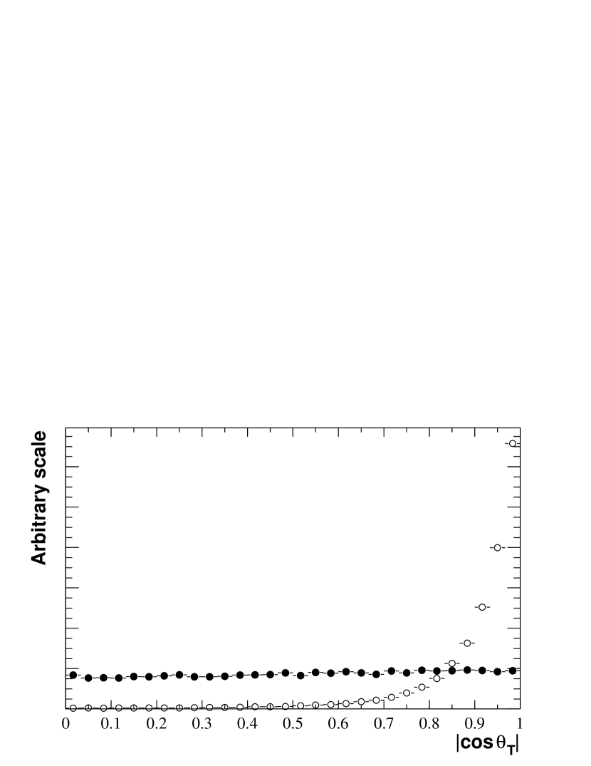
Figure 5: Distribution in $|\cos\theta_{\rm T}|$ for a typical $B$ meson decay ($B^{0}\rightarrow\eta^{\prime}_{\rho\gamma}\pi^{0}$ MC, solid points) and for the corresponding continuum background data (open circles).

Further use of the event topology is made via the construction of a Fisher discriminant ${\cal F}$, which is subsequently used as a discriminating variable in the likelihood fit. The Fisher discriminant we use is an optimized linear combination of the remaining event shape information (excluding $\cos\theta_{\rm T}$, which we have already used in our preselection requirements). The variables entering the Fisher discriminant are the angles with respect to the beam axis of the $B$ momentum and $B$ thrust axis (in the $\mathchar 28935\relax(4S)$ frame), and the zeroth and second angular moments $L_{0,2}$ of the energy flow about the $B$ thrust axis. The moments are defined by $L_{j}=\sum_{i}p_{i}\times\left|\cos\theta_{i}\right|^{j},$ where $\theta_{i}$ is the angle with respect to the $B$ thrust axis of track or neutral cluster $i$, $p_{i}$ is its momentum, and the sum excludes the $B$ candidate. The coefficients used to combine these variables are chosen to maximize the separation (difference of means divided by quadrature sum of errors) between the signal and continuum background distributions of $L_{j}$, and are determined from studies of signal MC and off-peak data. We have studied the optimization of ${\cal F}$ for a variety of signal modes, and find that the optimal sets of coefficients are nearly identical for all. Thus we do not re-optimize the Fisher coefficients for each individual decay. Because the information contained in ${\cal F}$ is correlated with $|\cos\theta_{\rm T}|$, the separation between signal and background is dependent on the $|\cos\theta_{\rm T}|$ requirement made prior to the formation of ${\cal F}$. In Fig. 6, we show the Fisher-discriminant distribution for signal and continuum background for the $B^{-}\rightarrow D^{0}\pi^{-}$ control sample.

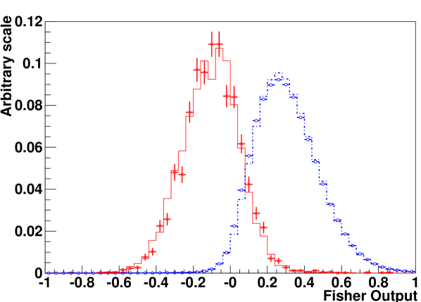
Figure 6: Distributions of Fisher-discriminant output for the data control mode $B^{-}\rightarrow D^{0}\pi^{-},\;D^{0}\rightarrow K^{-}\pi^{+}\pi^{0}$ (points with error bars), corresponding signal Monte Carlo (solid histogram), continuum data (open circles) and continuum Monte Carlo (dashed histogram) after requiring $|\cos\theta_{\rm T}|<0.9$. The Fisher discriminant and $|\cos\theta_{\rm T}|$ are strongly correlated, so the separation depends on this requirement.

IV.3 $B\kern 1.79993pt\overline{\kern-1.79993ptB}{}$ backgrounds

Most charmless hadronic-$B$-decay analyses do not have much background from other $B$ decays. Specifically, since most $B$ mesons decay via $b\rightarrow c$ transitions, the strange and light meson decay products from such decays result from $b\rightarrow c\rightarrow q$ cascades, and thus have lower momentum than those expected in the signal final states. This small background is included in our $q\overline{q}$ background PDF shapes (see next section) since the shapes are extracted from on-peak data.

We have found, however, that some of the signal modes (see Table 2 in Sec. IX) do suffer from backgrounds from charmless hadronic decay modes. We investigate backgrounds that may not be completely suppressed by the selection criteria defined in Sec. III with Monte Carlo samples of $B\kern 1.79993pt\overline{\kern-1.79993ptB}{}$ events corresponding to several times the number of such events in the dataset. When we find an indication of a high selection rate for a particular background decay mode, we use the experimentally measured (when available) or theoretically predicted branching fraction of that mode to determine its expected contribution. Fits to simulated experiments such as those described in Sec. VII are used to evaluate whether such events cause a significant bias to the measured signal yield. Based on these studies, we have adjusted (while still blind) some selection criteria and in some cases added a component to the ML fit to account explicitly for the remaining $B\kern 1.79993pt\overline{\kern-1.79993ptB}{}$  background contributions. Systematic errors account for the uncertainties in this method. The details of this procedure are described below.

V Maximum Likelihood Fit

We use an unbinned, extended maximum likelihood fit to extract signal yields for our modes. A subsample of events to fit for each decay channel is selected as described in Sec. III. The sample sizes for the decay chains reported here range from 700 to 30,000 events, where we include sidebands in all discriminating variables in order to parameterize the backgrounds.

V.1 Likelihood function

The likelihood function incorporates several discriminating variables to distinguish signal from the large number of background events retained by the sample selection. We describe the $B$-decay kinematics with two variables: $\Delta E$ and $m_{\rm ES}$ (as defined in Sec. III.6). We also include the mass of the primary resonance candidate ($m_{\eta}$, $m_{\eta^{\prime}}$, $m_{K^{*}}$, $m_{\rho}$, $m_{{\omega}}$, or $m_{\phi}$) and the Fisher discriminant ${\cal F}$. For the vector-pseudoscalar modes with a $K^{*}$, $\rho$, ${\omega}$, or $\phi$, we also include in the fit the helicity cosine ${\cal H}$ of the vector meson. For the $K^{*}$, $\rho$, and $\phi$, ${\cal H}$ is defined in Sec. III.5. For the $B^{0}\rightarrow\omega\pi^{0}$ decay, ${\cal H}$ is defined as the cosine of the angle between the normal to the $\omega$ decay plane (the plane of the three pions in the $\omega$ rest frame) and the flight direction of the $\omega$, measured in the $\omega$ rest frame.

Because correlations among the discriminating variables (except resonance mass and ${\cal H}$ for background) in the selected data are small, we take the probability distribution function (PDF) for each event $i$ to be a product of the PDFs for the separate discriminating variables. We define hypotheses $j$, where $j$ can be signal, continuum background, or (where appropriate) $B\kern 1.79993pt\overline{\kern-1.79993ptB}{}$ background. The PDFs can be written as

$${\cal P}^{i}_{j}={\cal P}_{j}(m_{ES}^{i}){\cal P}_{j}(\Delta E^{i}){\cal P}_{j}({\cal F}^{i}){\cal P}_{j}(m^{i}_{P}){\cal P}_{j}(m^{i}_{V},{\cal H}^{i}),$$ (6)

where $m_{P}$ indicates the pseudoscalar candidate mass in the fit (absent for $B^{0}\rightarrow\omega\pi^{0}$ and $B^{0}\rightarrow\phi\pi^{0}$ modes) and $m_{V}$ indicates the vector candidate mass (absent for the $\eta^{(\prime)}\pi^{0}$ modes).

The likelihood function for each decay mode is

$${\cal L}=\frac{\exp{(-\sum_{j}Y_{j})}}{N!}\prod_{i}^{N}\sum_{j}Y_{j}{\cal P}^{i}_{j}\,,$$ (7)

where $Y_{j}$ is the yield of events for hypothesis $j$ (to be found by the fitter) and $N$ is the observed number of events in the sample. The first factor takes into account the Poisson fluctuations in the total number of events.

VI Signal and background model

We determine the PDFs for signal from MC distributions for each discriminating variable. The PDFs for $B\kern 1.79993pt\overline{\kern-1.79993ptB}{}$ background (where appropriate) arise from fitting the composite $B\kern 1.79993pt\overline{\kern-1.79993ptB}{}$ MC sample, described in Sec. VI.1. For the continuum background we establish the functional forms and initial parameter values of the PDFs with data from sidebands in $m_{\rm ES}$ or $\Delta E$. We then refine the main background parameters (excluding resonance-mass central values and widths) by allowing them to float in the final fit so that they are determined by the full data sample. The following sections describe first the construction of samples to represent $B\kern 1.79993pt\overline{\kern-1.79993ptB}{}$ background, and then the control samples used to validate the PDF shapes and make adjustments to the means and widths of the distributions where needed. Finally we describe the detailed functional forms used to parameterize all of the signal and background distributions.

VI.1 Inclusion of $B\kern 1.79993pt\overline{\kern-1.79993ptB}{}$ background in the fits

As discussed in Sec. IV.3, backgrounds from other charmless $B$ decays need to be accounted for explicitly in the maximum likelihood fit for some decay chains.

Since we find that the signal yield bias due to $B\kern 1.79993pt\overline{\kern-1.79993ptB}{}$ background for the $\eta_{3\pi}$$K^{*}$ channels is less than 1% of the signal yield, we do not include a $B\kern 1.79993pt\overline{\kern-1.79993ptB}{}$ component for these modes. For all modes with a $K^{*+}\rightarrow K^{+}\pi^{0}$ decay, nearly all $B\kern 1.79993pt\overline{\kern-1.79993ptB}{}$ backgrounds are removed by the requirement ${\cal H}>-0.5$. This requirement is also helpful in reducing the $B\kern 1.79993pt\overline{\kern-1.79993ptB}{}$ background for decays with a $\rho^{+}\rightarrow\pi^{+}\pi^{0}$, though sufficient background remains to be included in the fit. For all other modes except $B^{0}\rightarrow\phi\pi^{0}$, we include a $B\kern 1.79993pt\overline{\kern-1.79993ptB}{}$ component in the fit. The fit number of $B\kern 1.79993pt\overline{\kern-1.79993ptB}{}$ events is a small fraction of the total sample and is tabulated in Table 2 in Sec. IX.

The PDFs for $B\kern 1.79993pt\overline{\kern-1.79993ptB}{}$ background are determined by fitting a sample of MC events composed of several charmless decay chains, with the PDF shapes described below. For the $\eta\rightarrow\gamma\gamma$ channels, the $B\kern 1.79993pt\overline{\kern-1.79993ptB}{}$ background is dominated by $B\rightarrow K^{*}\gamma$ decays, even after the $\eta$ decay angle requirement, due to the relatively large $K^{*}\gamma$ branching fraction ($40\times 10^{-6}$). For the $B\rightarrow\eta\rho$ channels, the largest backgrounds are from $\eta K^{*}$ decays, with misidentification of the charged kaon or loss of the kaon while selecting a pion from the other $B$. For the $\eta^{\prime}$ channels, the dominant backgrounds in all modes, except for $\eta^{\prime}_{\rho\gamma}\rho$, arise from $B\rightarrow\eta^{\prime}K$ decays, due to the relatively large branching fraction ($\sim 70\times 10^{-6}$). Another important background for the $\eta^{\prime}_{\rho\gamma}$$K^{*}$ channels, is $K^{*}\rho^{0}$ decays, where the $\rho$ is combined with a photon to fake an $\eta^{\prime}$. For the $\eta^{\prime}_{\rho\gamma}\rho$ and $\eta^{\prime}_{\rho\gamma}\pi^{0}$ modes, $B\kern 1.79993pt\overline{\kern-1.79993ptB}{}$  backgrounds are primarily from $B^{+}\rightarrow\rho^{+}\rho^{0}$ and $B^{0}\rightarrow\rho^{+}\rho^{-}$ decays. For the decays with a primary $\pi^{0}$, the largest backgrounds are from $B^{+}\rightarrow\eta^{(\prime)}\rho^{+}$ and $B^{+}\rightarrow\omega\rho^{+}$ decays, where due to the forward-backward peaking of the $\rho^{+}$ ${\cal H}$ distribution, the $\pi^{0}$ is often energetic and the charged pion is lost.

VI.2 PDF corrections from data control samples

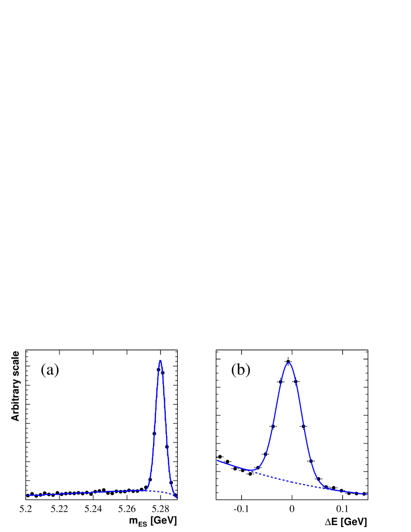
Figure 7: Distributions of (a) $m_{\rm ES}$ and (b) $\Delta E$ from the $B^{-}\rightarrow\pi^{-}D^{0}$ data sample used to determine the small corrections to signal Monte Carlo PDF shapes.

We validate the simulation on which we rely for signal PDFs by comparing critical distributions of discriminating variables in MC with those from large data control samples. For $m_{\rm ES}$ and $\Delta E$ (see Fig. 7), we use the decays $B^{-}\rightarrow\pi^{-}D^{0}~{}{\rm and}~{}B^{-}\rightarrow\rho^{-}D^{0}~{}{\rm with}~{}D^{0}\rightarrow K^{-}\pi^{+}\pi^{0}$, which have similar topology to the modes under study here. We select these samples by making loose requirements on $m_{\rm ES}$ and $\Delta E$, and more stringent selections on $\cos\theta_{\rm T}$ and the $D^{0}$ and $\rho$ candidate masses (as appropriate). We also place kinematic requirements on the $D$ and $B$ daughters to force the charmed decay to look as much like that of a charmless decay as possible without eliminating the control-sample signal. These selection criteria are applied both to the data and to a MC mixture of related $B\rightarrow DX$ and $B\rightarrow D^{*}X$ decays, which simulates the crossfeed from $D^{*}\rightarrow D^{0}$ decays observed in data. From these control samples, we determine small adjustments to the mean value of the signal $m_{\rm ES}$ distribution and to the resolution of the $\Delta E$ distribution compared with Monte Carlo. For ${\cal F}$ we use parameters found from a sample of approximately 500 $B^{+}\rightarrow\eta^{\prime}_{\rho\gamma}K^{+}$ events, with a $\cos\theta_{\rm T}$ requirement matching that used for each signal mode.

For the mass shapes of the resonances, we study inclusive resonance production in the off-peak data and corresponding continuum MC. In each sample, we reconstruct resonance candidates involved in our final states, requiring a minimum value of the candidate CM momentum of 1.9 $\mathrm{\,Ge\kern-1.00006ptV}$ to reflect the kinematics of our final states. The resolutions and means of the invariant mass distributions are compared, and we adjust the means and widths of PDF parameterizations based on the outcome of these results. A typical mass distribution for each resonance is shown in Fig. 8.

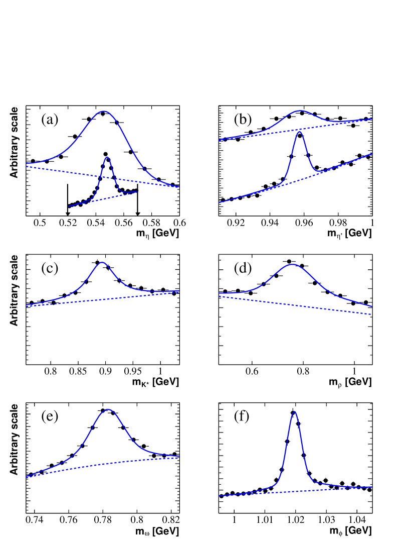
Figure 8: Distributions of the candidate masses for resonant decays from the on-peak sideband samples in data that are used to describe the signal PDF shapes (see Secs. VI.6 and VI.7). For each distribution a real resonance signal component is evident above a combinatorial background component: (a and b) the four $\eta^{(\prime)}$ candidate mass combinations from the $\eta\rho$ and $\eta^{\prime}\rho$ samples; (c) $K^{*}$ candidate mass from the $\eta^{\prime}_{\rho\gamma}K^{*}$ sample; (d) primary $\rho$ candidate mass from the $\eta^{\prime}_{\rho\gamma}\rho$ sample; (e) ${\omega}$ candidate mass from the $\omega\pi^{0}$ sample; (f) $\phi$ candidate mass from the $\phi\pi^{0}$ sample. In (a) the arrows indicate the narrower mass requirement for the $\eta\rightarrow\pi^{+}\pi^{-}\pi^{0}$ decay. The same range is used even for the narrower $\eta^{\prime}\rightarrow\eta\pi^{+}\pi^{-}$ distribution, shown as the lower plots in (b). For the $K^{*}$ and $\rho$ cases, we do not show both charges since the distributions are very similar.

VI.3 $m_{\rm ES}$ parameterization

The signal distribution in $m_{\rm ES}$ is parameterized by two Gaussian functions centered near the mass of the $B$ meson. The second Gaussian typically accounts for less than 20% of the total area, and has a larger width to take into account the tails of the distribution, which arise primarily from misreconstructed signal events. In continuum background, we model $m_{\rm ES}$ by a phase-space-motivated empirical function argus of the form

$$f(x)\propto x\sqrt{1-x^{2}}\exp{\left[-\xi(1-x^{2})\right]}\,,$$ (8)

where we define $x\equiv 2\mbox{$m_{\rm ES}$}/\sqrt{s}$, and $\xi$ is a parameter determined by the fit. In $B\kern 1.79993pt\overline{\kern-1.79993ptB}{}$ background samples, we find that the $m_{\rm ES}$ distribution is well-described by adding a simple Gaussian function to the empirical shape in Eq. 8; a similar alternate form of a Gaussian convolved with an exponential is used for some channels.

VI.4 $\Delta E$ parameterization

For $\Delta E$, we fit the signal distribution with two Gaussian functions, both centered near zero. The broad Gaussian has a width about five times larger than the narrow Gaussian; this accounts for energy loss before or leakage out of the EMC, as well as incorrect candidate combinations in true signal events. The broad Gaussian component becomes larger as more of the final state energy is carried by neutral particles. The primary Gaussian function accounts for about (60–80)% of the total area in all modes except $\eta^{(\prime)}\rho$ where it is between 30% and 60%. For continuum background, we model the $\Delta E$ distribution with a linear or quadratic polynomial as required by the data. The $B\kern 1.79993pt\overline{\kern-1.79993ptB}{}$ background is described well by two Gaussian functions peaking at negative (positive) $\Delta E$, accounting for backgrounds that have a larger (smaller) number of tracks and neutrals in the final state than the signal.

VI.5 Fisher parameterization

For both signal and background, the Fisher distribution ${\cal F}$ is described well by a Gaussian function with different widths to the left and right of the mean. For the continuum background distribution, we also include a second Gaussian function with a larger width to account for a small tail in the signal ${\cal F}$ region. This additional component of the PDF is important, because it prevents the background probability from becoming infinitesimally small in the region where signal lies. As shown in Fig. 6, the mean of the continuum background distribution is approximately $2\sigma$ greater than the mean of the signal peak, allowing for strong discrimination between the two. Because ${\cal F}$ describes the overall shape of the event, the distribution for $B\kern 1.79993pt\overline{\kern-1.79993ptB}{}$ background is very similar to the signal distribution; hence this variable has little discriminating power against $B\kern 1.79993pt\overline{\kern-1.79993ptB}{}$ background.

VI.6 Pseudoscalar mass parameterization

The pseudoscalar candidate mass distributions for signal are described well by the sum of two Gaussian functions. We use MC values for the means and widths of these Gaussians, corrected where necessary by using samples such as those shown in Fig. 8. In continuum background, we fit the data with two Gaussian functions, where we fix the means and widths to those used for signal, and include a linear or quadratic term to account for non-resonant background. The fraction of resonant to non-resonant background is allowed to float in the final fit. When there is no discernible resonant component, as in $\eta^{\prime}\rightarrow\rho^{0}\gamma$, floating this parameter can cause convergence issues in the final ML fit. If validation studies show this effect, the resonant fraction is fixed in the final analysis. For $B\kern 1.79993pt\overline{\kern-1.79993ptB}{}$ background, we use the same functional form as in continuum background; whether or not there is a true resonant component in $B\kern 1.79993pt\overline{\kern-1.79993ptB}{}$  background depends upon the charmless decay chains expected to contribute.

VI.7 Vector mass and helicity parameterization

In pseudoscalar–vector decays of the $B$ meson, the vector meson has a helicity-angle distribution proportional to ${\cal H}^{2}$ for true signal events. We model the vector-meson helicity distribution for signal with a polynomial times a threshold function that allows for the effects of acceptance. The signal $K^{*}$ and ${\omega}$ invariant-mass distributions are described by Breit-Wigner shapes. The $\phi$ and $\rho$ line shapes are found to be modeled well by two Gaussian functions; these do not fit well to a Breit-Wigner shape because of non-negligible mass resolution ($\phi$) or misreconstructed $\rho$ candidates in real signal events ($\rho$). For the $\rho$ and other wide distributions there is as much as 10% loss of efficiency due to the effect of the mass range requirements; this effect is included in the overall efficiency estimate and its uncertainty is included in systematic errors discussed in Sec. X. See Fig. 8 for illustrations of these distributions.

Because the shape of the helicity angle can be different for continuum background with and without a true vector resonance, we use a two-dimensional PDF to describe the resonance mass distribution and the helicity-angle distribution. We would expect that the background ${\cal H}$ would have a nearly uniform distribution, corresponding to a sum of combinatorial resonance background and background of true resonances from various production mechanisms. We find that the pure-background shape is modeled well by a second order polynomial with only a small amount of curvature and the true-resonance component is a separate low-order-polynomial shape. The mass parameters for the true-resonance component are fixed to be the same as for the signal.

The $B\kern 1.79993pt\overline{\kern-1.79993ptB}{}$ background component of ${\cal H}$ is modeled by a single fourth-degree polynomial. We parameterize the resonance mass distribution with two Gaussian functions plus a linear or quadratic polynomial, allowing the means and widths of the Gaussians to float if the resonant component of the background differs from the signal resonance. This is especially necessary when $B\kern 1.79993pt\overline{\kern-1.79993ptB}{}$ background arises when a misidentified kaon from a $K^{*}$ causes its reconstruction as a $\rho$.

The requirement that charged tracks have $p_{T}>100$ $\mathrm{\,Me\kern-1.00006ptV}$  (Sec. III) can induce a “roll-off” effect near ${\cal H}$ values of $\pm 1$. In particular, for decays of a $K^{*}$ or $\rho$ with a charged pion, the helicity distribution of the vector meson shows a characteristic roll-off in the region populated by low-momentum pions. This effect is absent for charged kaons since there are no kaons with $p_{T}<100$ $\mathrm{\,Me\kern-1.00006ptV}$. We model the roll-off in both the signal and background ${\cal H}$ distributions by multiplying the primary PDF shape by an appropriate Fermi-Dirac threshold function. The parameters of this roll-off function are constrained to be the same for signal and both background components. Because the ${\omega}$ helicity angle is defined from a three-body decay (${\omega\rightarrow\pi^{+}\pi^{-}\pi^{0}}$), there is little correlation between low-momentum pions and helicity angle, and hence no significant roll-off.

VII Fit Validation

Before applying the fitting procedure to the data to extract the signal yields we subject it to several tests. Internal consistency is checked with fits to ensembles of “experiments” generated by Monte Carlo from the PDFs. From these we establish the number of parameters associated with the PDF shapes that can be left free in addition to the yields. Ensemble distributions of the fitted parameters verify that the generated values are reproduced with the expected resolution. The ensemble distribution of $\ln{{\cal L}}$ itself provides a reference to check the goodness of fit of the final measurement once it has been performed.

We account for possible biases due to neglecting correlations among discriminating variables in the PDFs by fitting ensembles of experiments into which we have embedded the expected number of signal events randomly extracted from the detailed MC samples, where correlations are modeled fully. We find a positive bias of a few events for most modes, as shown in Table 1. Events from a weighted mixture of simulated $B\kern 1.79993pt\overline{\kern-1.79993ptB}{}$  background decays are included where significant, and so the bias we measure includes the effect of crossfeed from these modes.

Table 1: For each $B$ decay chain we present the optimized $|\cos\theta_{\rm T}|$ requirement, the number of on-peak events passing the preselection requirements, and the fit bias $Y_{b}$ determined from simulated experiments (the uncertainty on this bias is discussed in Sec. X).

Mode	Max $|\cos\theta_{\rm T}|$	#Events	Fit bias, $Y_{b}$
		in fit	(events)
$B^{+}\rightarrow\eta K^{*+}$
$\eta_{\gamma\gamma}K^{*+}_{K^{0}\pi^{+}}$	0.90	7573	$-$4.7
$\eta_{3\pi}K^{*+}_{K^{0}\pi^{+}}$	0.90	4132	$-$1.7
$\eta_{\gamma\gamma}K^{*+}_{K^{+}\pi^{0}}$	0.90	4974	$-$0.1
$\eta_{3\pi}K^{*+}_{K^{+}\pi^{0}}$	0.90	2835	$-$0.3
$B^{0}\rightarrow\eta K^{*0}$
$\eta_{\gamma\gamma}K^{*0}$	0.90	12179	$-$8.1
$\eta_{3\pi}K^{*0}$	0.90	6440	$-$1.8
$B^{+}\rightarrow\eta\rho^{+}$
$\eta_{\gamma\gamma}\rho^{+}$	0.80	17084	$-$1.3
$\eta_{3\pi}\rho^{+}$	0.90	16106	$-$1.0
$B^{0}\rightarrow\eta\rho^{0}$
$\eta_{\gamma\gamma}\rho^{0}$	0.70	11107	$-1.0$
$\eta_{3\pi}\rho^{0}$	0.80	8347	$-$2.3
$B^{0}\rightarrow\eta\pi^{0}$
$\eta_{\gamma\gamma}\pi^{0}$	0.80	5379	$-1.1$
$\eta_{3\pi}\pi^{0}$	0.80	2271	$-$0.7
$B^{+}\rightarrow\eta^{\prime}K^{*+}$
$\eta^{\prime}_{\eta\pi\pi}K^{*+}_{K^{0}\pi^{+}}$	0.90	2973	$-4.5$
$\eta^{\prime}_{\rho\gamma}K^{*+}_{K^{0}\pi^{+}}$	0.75	13299	$-$3.6
$\eta^{\prime}_{\eta\pi\pi}K^{*+}_{K^{+}\pi^{0}}$	0.90	2009	$-$0.0
$\eta^{\prime}_{\rho\gamma}K^{*+}_{K^{+}\pi^{0}}$	0.75	8205	$-$0.6
$B^{0}\rightarrow\eta^{\prime}K^{*0}$
$\eta^{\prime}_{\eta(\gamma\gamma)\pi\pi}K^{*0}$	0.90	4808	$-3.7$
$\eta^{\prime}_{\eta(3\pi)\pi\pi}K^{*0}$	0.90	695	$-$1.7
$\eta^{\prime}_{\rho\gamma}K^{*0}$	0.75	20504	$-$4.2
$B^{+}\rightarrow\eta^{\prime}\rho^{+}$
$\eta^{\prime}_{\eta\pi\pi}\rho^{+}$	0.90	8737	$-$2.1
$\eta^{\prime}_{\rho\gamma}\rho^{+}$	0.65	28933	$-$7.8
$B^{0}\rightarrow\eta^{\prime}\rho^{0}$	0.90	9515	$-3.7$
$B^{0}\rightarrow\eta^{\prime}\pi^{0}$
$\eta^{\prime}_{\eta\pi\pi}\pi^{0}$	0.90	3491	$-3.5$
$\eta^{\prime}_{\rho\gamma}\pi^{0}$	0.70	11426	$-$2.8
$B^{0}\rightarrow\omega\pi^{0}$	0.80	18986	$-2.1$
$B^{0}\rightarrow\phi\pi^{0}$	0.90	4840	$-1.1$

For modes with low background and small signal yields, the ensemble yield distribution may exhibit a significant negative tail. This is due to the nature of the maximum likelihood method, which is known to be biased for small samples. The source of the bias is the insufficient number of events for which the probability for the signal hypothesis is larger than the probability for the background hypothesis. This results in a negative bias, which is taken as the mean of the yield distribution from the fits to the ensembles described above. Examples of modes with negative bias can be found in Table 1. By subtracting the bias we correct for this effect on average, and we include the uncertainty as a systematic error.

This same procedure for generating and fitting simplified MC samples is used to find an optimal selection requirement for the $\cos\theta_{\rm T}$ variable in the early stages of each analysis. The studies are performed for a range of selection values, to minimize the fractional error on the signal yield. The optimal values of the $\cos\theta_{\rm T}$ requirement that are chosen are given in Table 1.

Finally, we apply the fit to the off-peak data to confirm that we find no fake signals in a sample with no signal events.

VIII Efficiencies and Efficiency Corrections

The efficiency is determined by the ratio of the number of signal Monte Carlo events passing preselection to the total number of generated MC signal events. This efficiency is corrected for differences between the true detector efficiencies and those simulated in Monte Carlo. From a study of absolute tracking efficiency, we apply a correction of (1–7)%, depending on the number of charged particles in the decay channel and assign a systematic error of 0.8% per track. The $K^{0}_{\scriptscriptstyle S}$ efficiency correction is taken from an independent study of the vertex-displacement dependence of the efficiency for inclusive samples of $K^{0}_{\scriptscriptstyle S}$ mesons from the data and from MC. The overall correction for the topologies represented by our decays is $0.971\pm 0.030$. For the six decays with a primary $\pi^{0}$ and the four with a $K^{*+}$ or $\rho^{+}$ decaying to a final state with an energetic $\pi^{0}$, we determine a correction from a sample of tau decays. For these cases, the $\pi^{0}$ efficiency is 6–11% lower for data than MC.

IX Fit Results

The branching fraction for each decay chain is obtained from

$${\cal B}=\frac{Y-Y_{b}}{\epsilon\prod{{\cal B}_{i}}N_{B}}\,,$$ (9)

where $Y$ is the yield of signal events from the fit, $Y_{b}$ is the fit bias discussed in Sec. VII and given in Table 1, $\epsilon$ is the efficiency, ${\cal B}_{i}$ is the branching fraction for the $i$th unstable $B$ daughter (${\cal B}_{i}$ having been set to unity in the MC simulation), and $N_{B}$ is the number of produced $B^{+}$ or $B^{0}$ mesons. The values of ${\cal B}_{i}$ are taken from Particle Data Group world averages PDG2002 . The number of produced $B$ mesons is computed with the assumption of equal production rates of charged and neutral $B$  pairs bbRpluszero .

In Table 2, we show the results of the final ML fits to the on-peak data, with the yields for signal and $B\kern 1.79993pt\overline{\kern-1.79993ptB}{}$ background, where applicable. The latter is often uncertain due to the large correlation with the $q\overline{q}$ background component, but this uncertainty is not problematic because the correlation with signal is small. We also show the efficiencies, daughter branching-fraction products, and estimated effective purity of the sample. We report the statistical significance for the individual decay chains and display the significance including systematic uncertainties for the combined result in each channel. The purity is the ratio of the signal yield to the effective background plus signal; we estimate the denominator by taking the square of the uncertainty of the signal yield as the sum of effective background plus signal. Where the signal yields are small the purity is not very meaningful, so we do not report the purity if it is below 10%. Branching fractions are given for individual fits to each submode as well as the result of combining several submodes. Since the latter procedure involves systematic as well as statistical errors, we defer the description to Sec. XI. The final column in Table 2 gives the charge asymmetry (${\cal A}_{ch}$), as defined in Sec. I.

Table 2: Fitted event yields ($Y=$ signal yield, $Y_{B\kern 1.25995pt\overline{\kern-1.25995ptB}{}}=$ $B\kern 1.79993pt\overline{\kern-1.79993ptB}{}$ yield), purity ($P$, see text), efficiency ($\epsilon$), daughter product branching fractions (in percent), significance ${\cal S}(\sigma)$ (which includes systematic errors), fit branching fractions, 90% C.L. upper limits, and charge asymmetries. Also shown are the results of combining daughter decay chains where more than one contribute. For the final branching fraction and charge asymmetry results, the systematic errors are also given.

Mode	$Y$	$Y_{B\kern 1.25995pt\overline{\kern-1.25995ptB}{}}$	$P$(%)	$\epsilon$	$\prod{\cal B}_{i}$	${\cal S}(\sigma$)	${\cal B}(10^{-6})$	UL $(10^{-6})$	${\cal A}_{ch}$
$B^{+}\rightarrow\eta K^{*+}$						$9$	$25.6\pm 4.0\pm 2.4$		$+0.13\pm 0.14\pm 0.02$
$\eta_{\gamma\gamma}K^{*+}_{K^{0}\pi^{+}}$	$46\pm 12$	$25\pm 15$	35	24.0	$9.0~{}~{}$	4.9	$22\pm 6$		$+0.03\pm 0.24$
$\eta_{3\pi}K^{*+}_{K^{0}\pi^{+}}$	$27\pm 8$		45	17.1	$5.2~{}~{}$	5.0	$33\pm 10$		$+0.46^{+0.24}_{-0.28}$
$\eta_{\gamma\gamma}K^{*+}_{K^{+}\pi^{0}}$	$30\pm 9$		45	8.8	$13.1~{}~{}$	5.7	$29\pm 8$		$-0.11\pm 0.28$
$\eta_{3\pi}K^{*+}_{K^{+}\pi^{0}}$	$10\pm 5$		43	6.6	$7.5~{}~{}$	3.2	$22\pm 11$		$+0.37^{+0.42}_{-0.51}$
$B^{0}\rightarrow\eta K^{*0}$						$11$	$18.6\pm 2.3\pm 1.2$		$+0.02\pm 0.11\pm 0.02$
$\eta_{\gamma\gamma}K^{*0}$	$125\pm 16$	$5\pm 19$	50	24.4	$26.3~{}~{}$	10.1	$20\pm 3$		$+0.12\pm 0.13$
$\eta_{3\pi}K^{*0}$	$32\pm 9$		47	16.5	$15.1~{}~{}$	5.0	$14\pm 4$		$-0.39\pm 0.25$
$B^{+}\rightarrow\eta\rho^{+}$						$3.5$	$9.2\pm 3.4\pm 1.0$	$<$$14$
$\eta_{\gamma\gamma}\rho^{+}$	$32\pm 15$	$-3\pm 19$	14	10.7	$39.4~{}~{}$	2.5	$8\pm 4$
$\eta_{3\pi}\rho^{+}$	$21\pm 11$	$3\pm 11$	17	8.6	$22.6~{}~{}$	2.4	$12\pm 6$
$B^{0}\rightarrow\eta\rho^{0}$						$-$	$-1.1^{+0.7}_{-0.9}\pm 0.4$	$<$$1.5$
$\eta_{\gamma\gamma}\rho^{0}$	$-18\pm 18$	$67\pm 38$	$<$10	27.1	$39.4~{}~{}$	$-$	$-2\pm 2$
$\eta_{3\pi}\rho^{0}$	$-2\pm 4$	$26\pm 10$	$<$10	18.2	$22.6~{}~{}$	$-$	$-1\pm 1$
$B^{0}\rightarrow\eta\pi^{0}$						$0.8$	$0.7^{+1.1}_{-0.9}\pm 0.3$	$<$$2.5$
$\eta_{\gamma\gamma}\pi^{0}$	$1\pm 7$	$-2\pm 9$	$<$10	19.3	$39.4~{}~{}$	0.3	$0\pm 1$
$\eta_{3\pi}\pi^{0}$	$8\pm 7$	$-8\pm 5$	15	14.9	$22.6~{}~{}$	1.1	$2\pm 2$
$B^{+}\rightarrow\eta^{\prime}K^{*+}$						$1.9$	$6.3^{+4.6}_{-3.6}\pm 1.8$	$<$$14$
$\eta^{\prime}_{\eta\pi\pi}K^{*+}_{K^{0}\pi^{+}}$	$-8\pm 4$	$29\pm 11$	$<$10	17.5	$4.0~{}~{}$	$-$	$-5\pm 6$
$\eta^{\prime}_{\rho\gamma}K^{*+}_{K^{0}\pi^{+}}$	$16\pm 9$	$17\pm 12$	22	13.5	$6.8~{}~{}$	1.7	$~{}~{}15\pm 11$
$\eta^{\prime}_{\eta\pi\pi}K^{*+}_{K^{+}\pi^{0}}$	$~{}3\pm 3$		13	7.0	$5.8~{}~{}$	1.7	$~{}~{}8\pm 7$
$\eta^{\prime}_{\rho\gamma}K^{*+}_{K^{+}\pi^{0}}$	$~{}5\pm 7$		$<$10	5.6	$9.8~{}~{}$	0.6	$~{}~{}8\pm 14$
$B^{0}\rightarrow\eta^{\prime}K^{*0}$						$2.1$	$4.1^{+2.1}_{-1.8}\pm 1.2$	$<$$7.6$
$\eta^{\prime}_{\eta(\gamma\gamma)\pi\pi}K^{*0}$	$0\pm 4$	$18\pm 10$	$<$10	17.8	$11.6~{}~{}$	1.0	$2\pm 2$
$\eta^{\prime}_{\eta(3\pi)\pi\pi}K^{*0}$	$~{}11\pm 5$	$18\pm 9$	47	12.2	$6.7~{}~{}$	2.0	$13\pm 7$
$\eta^{\prime}_{\rho\gamma}K^{*0}$	$~{}~{}15\pm 10$	$80\pm 25$	17	14.0	$19.7~{}~{}$	1.3	$5\pm 4$
$B^{+}\rightarrow\eta^{\prime}\rho^{+}$						$2.6$	$12.9^{+6.2}_{-5.5}\pm 2.0$	$<$$22$
$\eta^{\prime}_{\eta\pi\pi}\rho^{+}$	$16\pm 8$		25	8.4	$17.5~{}~{}$	2.1	$~{}11\pm 6$
$\eta^{\prime}_{\rho\gamma}\rho^{+}$	$48\pm 23$	$61\pm 100$	$<$10	6.5	$29.5~{}~{}$	1.7	$~{}24\pm 13$
$B^{0}\rightarrow\eta^{\prime}\rho^{0}$	$-1\pm 4$	$53\pm 21$	$<$10	19.7	$17.5~{}~{}$	$0.5$	$0.8^{+1.7}_{-1.2}\pm 0.9$	$<$$4.3$
$B^{0}\rightarrow\eta^{\prime}\pi^{0}$						$0.7$	$1.0^{+1.4}_{-1.0}\pm 0.8$	$<$$3.7$
$\eta^{\prime}_{\eta\pi\pi}\pi^{0}$	$-2\pm 3$	$-8\pm 4$	$<$10	18.5	$17.5~{}~{}$	0.4	$1\pm 1$
$\eta^{\prime}_{\rho\gamma}\pi^{0}$	$17\pm 14$	$-38\pm 78$	$<$10	13.9	$29.5~{}~{}$	1.1	$4\pm 4$
$B^{0}\rightarrow\omega\pi^{0}$	$-9\pm 8$	$9\pm 18$	$<$10	15.9	$89.1~{}~{}$		$-0.6^{+0.7}_{-0.5}\pm 0.2$	$<$$1.2$
$B^{0}\rightarrow\phi\pi^{0}$	$2\pm 4$		$<$10	28.6	$49.2~{}~{}$	$0.7$	$0.2^{+0.4}_{-0.3}\pm 0.1$	$<$$1.0$

The statistical error on the yield is given by the change in the central value when the quantity $-2\ln{\cal L}$ increases by one unit. The statistical significance is taken as the square root of the difference between the value of $-2\ln{\cal L}$ for zero signal and the value at its minimum. The 90% C.L. upper limit quoted in Sec. XIII is the solution ${\cal B}_{90}$ to the equation

$$\frac{\int_{0}^{{\cal B}_{90}}{{\cal L}}(b)db}{\int_{0}^{\infty}{\cal L}(b)db}=0.9\,,$$ (10)

where ${\cal L}(b)$ is the value of the maximum likelihood for branching fraction $b$.

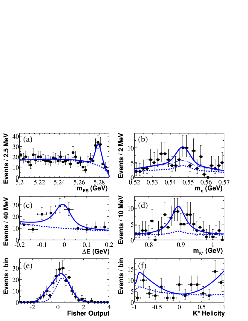
Figure 9: Projections of the $B$-candidate discriminating variables for $B^{+}\rightarrow\eta K^{*+}$: (a) $m_{\rm ES}$; (b) $\eta$ candidate mass; (c) $\Delta E$; (d) $K^{*+}$ candidate mass; (e) Fisher discriminant output; and (f) $K^{*+}$ helicity. See text for explanation of the points and curves.

In Figs. 9–11 we show projections of all fit discriminating variables for the $\eta K^{*}$ and $\eta\rho^{+}$ modes. Points with errors represent data, solid curves the full fit functions, and dashed curves the background functions. Since the $\eta\rightarrow\gamma\gamma$ and $\eta\rightarrow\pi^{+}\pi^{-}\pi^{0}$ components have very different resolutions, for the $\eta$-candidate mass plots we indicate with a dashed curve the full fit without the $\eta\rightarrow\pi^{+}\pi^{-}\pi^{0}$ signal component. We make these plots by selecting events with the ratio of signal to total likelihood (computed without the variable shown in the figure) exceeding a mode-dependent threshold that optimizes the expected sensitivity. The selection retains a fraction of the signal yield averaging about 70% across the decay sequences.

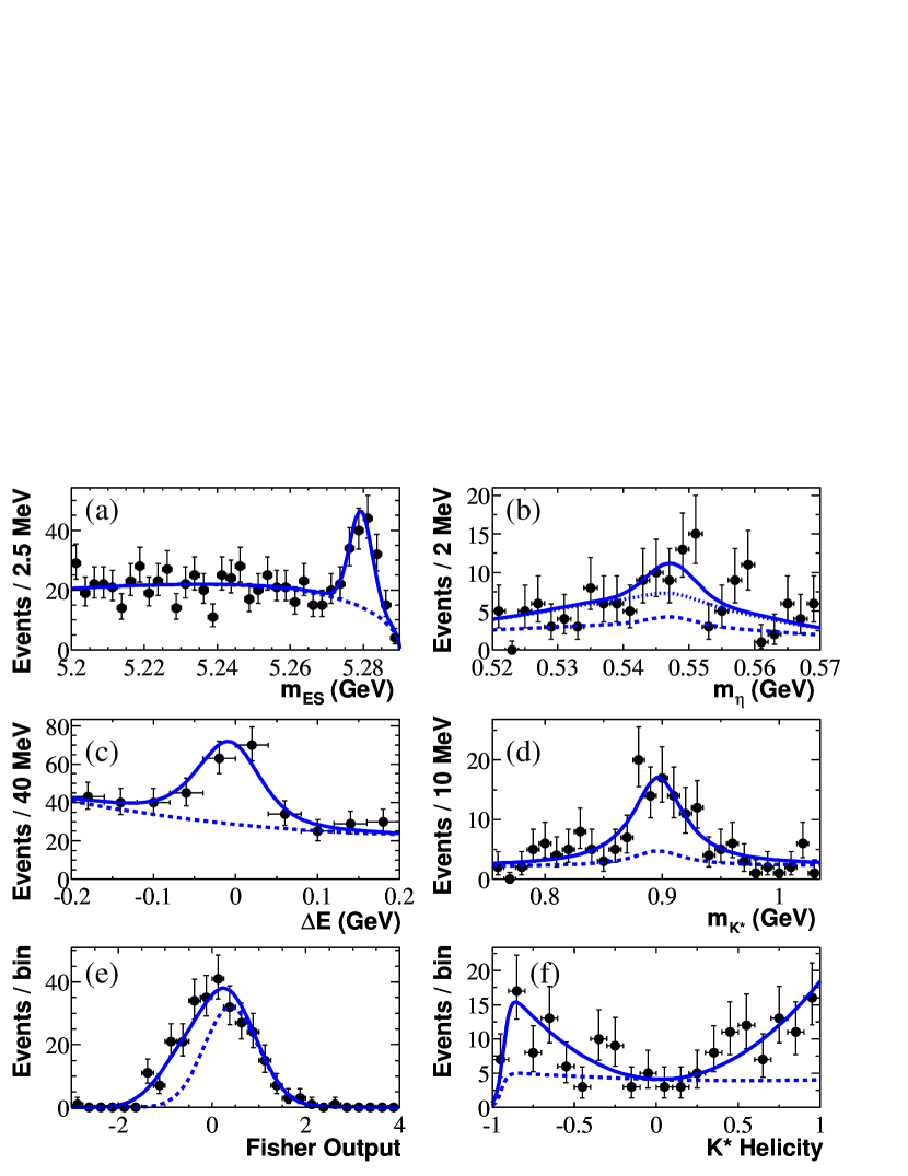
Figure 10: Projections of the $B$ candidate discriminating variables for $B^{0}\rightarrow\eta K^{*0}$: (a) $m_{\rm ES}$; (b) $\eta$ candidate mass; (c) $\Delta E$; (d) $K^{*0}$ candidate mass; (e) Fisher discriminant output; and (f) $K^{*0}$ helicity. See text for explanation of the points and curves.

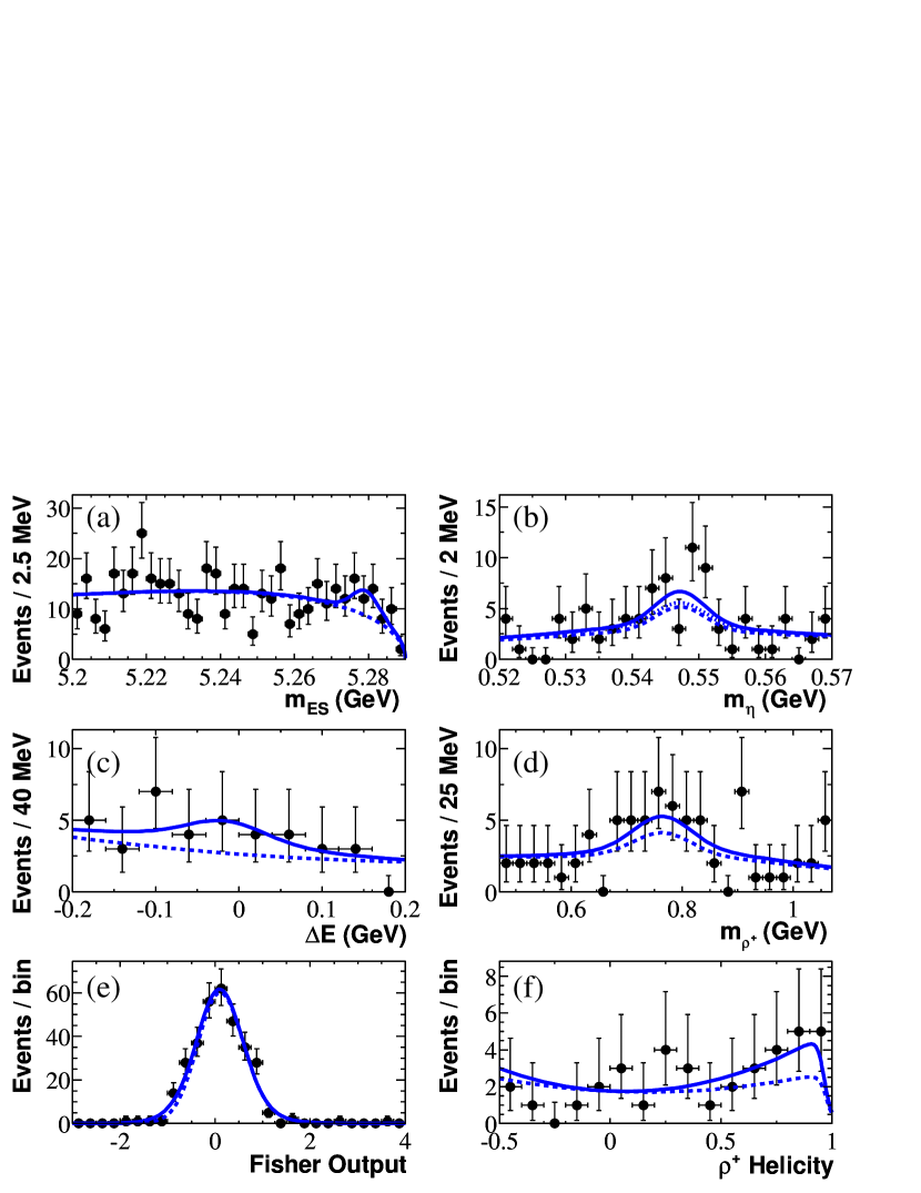
Figure 11: Projections of the $B$ candidate discriminating variables for $B^{+}\rightarrow\eta\rho^{+}$: (a) $m_{\rm ES}$; (b) $\eta$ candidate mass; (c) $\Delta E$; (d) $\rho^{+}$ candidate mass; (e) Fisher discriminant output; and (f) $\rho^{+}$ helicity. See text for explanation of the points and curves.

X Systematic Uncertainties

We itemize estimates of the various sources of systematic errors important for these measurements. Tables 3, 4, and 5 show the results of our evaluation of these uncertainties. We tabulate separately the additive and multiplicative uncertainties. That is, we distinguish those errors affecting the efficiency and total number of $B\kern 1.79993pt\overline{\kern-1.79993ptB}{}$ events from those that concern the bias of the yield, since only the latter affect the significance of the result. The two types of errors are comparable for modes with substantial yields but the additive errors dominate when the yields are small. Additionally we distinguish between those uncertainties that are correlated among different daughter decays of the same mode (C), and those that are uncorrelated (U). This distinction is relevant when multiple decay chains are combined (see Sec. XI). The final row of the table provides the total systematic error in the branching fraction for each of the submodes.

Table 3: Estimates of systematic uncertainties in the branching fraction for $B\rightarrow\eta K^{*}$ and $B\rightarrow\eta\rho$ decays. We distinguish between additive and multiplicative errors as well as errors that are correlated (C) or uncorrelated (U) among the submodes.

Quantity	$\eta K^{*+}$					$\eta K^{*0}$			$\eta\rho^{+}$		$\eta\rho^{0}$
$\eta$ decay	$\gamma\gamma$	$3\pi$	$\gamma\gamma$	$3\pi$		$\gamma\gamma$	$3\pi$		$\gamma\gamma$	$3\pi$   –	$\gamma\gamma$	$3\pi$
$K^{*}$, $\rho$ decay	$K^{0}\pi^{+}$	$K^{0}\pi^{+}$	$K^{+}\pi^{0}$	$K^{+}\pi^{0}$		$K^{+}\pi^{-}$	$K^{+}\pi^{-}$		$\pi^{+}\pi^{0}$	$\pi^{+}\pi^{0}$	$\pi^{+}\pi^{-}$	$\pi^{+}\pi^{-}$
Additive errors (events)
Fit yield (U)	2.1	0.7	0.4	0.3		2.2	2.3		2.3	0.2 –	5.2	0.9
Fit bias (U)	2.5	1.2	0.3	0.3		4.2	1.1		1.1	0.9 –	0.3	0.7
$B\kern 1.79993pt\overline{\kern-1.79993ptB}{}$ background (U)	1.1	0.3	0.6	0.5		0.9	0.3		0.7	0.4 –	6.5	1.2
Total additive (events)	3.4	1.4	0.6	0.5		4.8	2.6		2.6	1.0 –	8.1	1.6
Multiplicative errors (%)
Tracking eff/qual (C)	0.8	2.4	0.8	2.4		1.6	3.2		0.8	2.4 –	1.6	3.2
$K^{0}_{\scriptscriptstyle S}$ efficiency (C)	4.0	4.0
Track multiplicity (C)	1.0	1.0	1.0	1.0		1.0	1.0		1.0	1.0 –	1.0	1.0
$\pi^{0}$/ $\gamma$ eff (C)	5.1	5.1	10.3	10.3		5.1	5.1		10.3	10.3 –	5.1	5.1
Number $B\kern 1.79993pt\overline{\kern-1.79993ptB}{}$ (C)	1.1	1.1	1.1	1.1		1.1	1.1		1.1	1.1 –	1.1	1.1
Branching fractions (U)	0.7	1.8	0.7	1.8		0.7	1.8		0.7	1.8 –	0.7	1.8
MC statistics (U)	0.9	1.1	1.5	1.8		0.9	1.1		1.3	1.7 –	0.8	1.0
$\cos\theta_{\rm T}$ (C)	0.5	0.5	0.5	0.5		0.5	0.5		1.0	0.5 –	2.3	1.0
PID (C)			1.0	1.0		1.0	1.0
Total multiplicative (%)	6.8	7.4	10.6	11.0		5.8	6.6		10.6	11.0 –	6.1	6.6
Total $\sigma$ [${\cal B}(10^{-6}$)]	2.2	2.9	3.6	2.6		1.4	1.5		1.0	1.5 –	0.9	0.4

Table 4: Estimates of systematic uncertainties in the branching fraction for $B\rightarrow\eta^{\prime}K^{*}$ and $B\rightarrow\eta^{\prime}\rho$ decays. The notation is the same as for Table 3.

Quantity	$\eta^{\prime}K^{*+}$					$\eta^{\prime}K^{*0}$				$\eta^{\prime}\rho^{+}$			$\eta^{\prime}\rho^{0}$
$\eta^{\prime}$ decay	$\eta\pi\pi$	$\rho\gamma$	$\eta\pi\pi$	$\rho\gamma$		$\eta\pi\pi$	$\eta_{3\pi}\pi\pi$	$\rho\gamma$		$\eta\pi\pi$	$\rho\gamma$		$\eta\pi\pi$
$K^{*}$, $\rho$ decay	$K^{0}\pi^{+}$	$K^{0}\pi^{+}$	$K^{+}\pi^{0}$	$K^{+}\pi^{0}$		$K^{+}\pi^{-}$	$K^{+}\pi^{-}$	$K^{+}\pi^{-}$		$\pi^{+}\pi^{0}$	$\pi^{+}\pi^{0}$		$\pi^{+}\pi^{-}$
Additive errors (events)
Fit yield (U)	0.9	1.3	0.2	0.8		0.5	2.8	0.8		0.8	3.1		1.0
Fit bias (U)	2.3	1.9	0.3	0.4		1.7	0.8	2.1		1.2	4.3		1.9
$B\kern 1.79993pt\overline{\kern-1.79993ptB}{}$ background (U)	1.3	0.9	0.5	0.5		2.5	0.5	1.4		1.2	10.0		1.8
Total additive (events)	2.8	2.5	0.6	1.0		3.1	3.0	2.6		1.9	11.3		2.8
Multiplicative errors (%)
Tracking eff/qual (C)	2.4	2.4	2.4	2.4		3.2	4.8	3.2		2.4	2.4		3.2
$K^{0}_{\scriptscriptstyle S}$ efficiency (C)	4.0	4.0
Track multiplicity (C)	1.0	1.0	1.0	1.0		1.0	1.0	1.0		1.0	1.0		1.0
$\pi^{0}$/ $\gamma$ eff (C)	5.4	2.5	10.4	7.6		5.4	5.4	2.5		10.4	7.6		5.4
Number $B\kern 1.79993pt\overline{\kern-1.79993ptB}{}$ (C)	1.1	1.1	1.1	1.1		1.1	1.1	1.1		1.1	1.1		1.1
Branching fractions (U)	3.4	3.4	3.4	3.4		3.4	3.4	3.4		3.4	3.4		3.4
MC statistics (U)	1.0	1.2	1.7	1.9		1.1	1.1	1.1		1.5	1.8		0.9
$\cos\theta_{\rm T}$ (C)	0.5	1.8	0.5	1.8		0.5	1.4	1.4		0.5	3.0		0.5
PID (C)			1.0	1.0		1.0	1.0	1.0
Total multiplicative (%)	8.1	6.8	11.5	9.2		7.5	8.4	5.4		11.4	9.5		7.4
Total $\sigma$ [${\cal B}(10^{-6}$)]	4.5	3.2	1.9	2.1		1.7	4.2	1.1		1.9	6.9		0.9

Table 5: Estimates of systematic uncertainties in the branching fraction for the decays $B^{0}\rightarrow\eta\pi^{0}$, $B^{0}\rightarrow\eta^{\prime}\pi^{0}$, $B^{0}\rightarrow\omega\pi^{0}$ and $B^{0}\rightarrow\phi\pi^{0}$. The notation is the same as for Table 3.

Quantity	$\eta\pi^{0}$		$\eta^{\prime}\pi^{0}$		$\omega\pi^{0}$	$\phi\pi^{0}$
$\eta^{(\prime)}$ decay	$\gamma\gamma$	$3\pi$	$\eta\pi\pi$	$\rho\gamma$
Add. err. (evts.)
Fit yield (U)	1.0	1.3	1.2	2.8	1.4	0.8
Fit bias (U)	1.0	0.3	2.0	1.3	1.5	0.7
$B\kern 1.79993pt\overline{\kern-1.79993ptB}{}$ Bkg (U)	1.0	1.0	1.0	1.0	1.0	1.0
Total add. (evts.)	1.7	1.7	2.5	3.2	2.3	1.5
Mult. err. (%)
Track eff. (C)	0.0	1.6	1.6	1.6	1.6	1.6
Multiplicity (C)	1.0	1.0	1.0	1.0	1.0	1.0
$\pi^{0}$/ $\gamma$ eff (C)	14.9	11.5	13.1	9.1	11.7	7.9
Number $B\kern 1.79993pt\overline{\kern-1.79993ptB}{}$ (C)	1.1	1.1	1.1	1.1	1.1	1.1
Br. frac. (U)	0.8	1.8	3.4	3.4	0.8	1.4
MC stats. (U)	1.2	1.3	1.2	0.5	1.2	0.9
$\cos\theta_{\rm T}$ (C)	0.5	0.5	0.5	1.3	0.6	0.5
Total mult. (%)	15.1	11.9	13.8	10.1	12.0	8.4
Total $\sigma$ [${\cal B}(10^{-6}$)]	0.3	0.6	0.9	1.0	0.2	0.1

X.1 Additive systematic errors

Fit yield (U): Uncertainties due to imprecise knowledge of the background PDF parameters are included in the statistical errors since the main parameters are allowed to vary in the nominal fits. We have investigated the small correlations among background parameters and find these to have a negligible effect on signal yields. We include the uncertainty for the signal PDF parameters by determining the yield variations as individual parameters are varied by uncertainties determined from fits to independent control samples (see Sec. VI.2).

Fit bias (U): This uncertainty is taken from the validation procedure described in Sec. VII. We combine in quadrature terms, in order of relative importance, from (a) the positive bias (due to parameter correlations), (b) the negative bias for small event yields, (c) a small contribution from the modeling of the combinatorial component in signal, and (d) the statistical uncertainty in the determination of the bias. The first uncertainty (a) is taken to be one half of the positive bias, and the second (b) to be one half of the difference between the peak and mean yields of the ensemble distributions. Contribution (c) is small for all modes; we determine it using a comparison of Monte Carlo and data for the $B^{-}\rightarrow\pi^{-}D^{0}$ control sample.

$B\kern 1.79993pt\overline{\kern-1.79993ptB}{}$ background (U): The $B\kern 1.79993pt\overline{\kern-1.79993ptB}{}$ background component, included in the fit for most decay chains, accounts for most uncertainties from $B\kern 1.79993pt\overline{\kern-1.79993ptB}{}$ background. We assign an additional uncertainty to account for modeling of this background. For the high-background $\eta^{\prime}\rho^{+}$ decay this involves explicit variation of the model. For the other modes it is taken to be 50% of the difference in the signal yields when background is varied by its uncertainty (100% of the estimated effect when a $B\kern 1.79993pt\overline{\kern-1.79993ptB}{}$ background component is not included in the fit) and a contribution to account for uncertainty in the effect of the $b\rightarrow c$ background.

X.2 Multiplicative systematic errors

Track finding/efficiency (C): As described in Sec. VIII, we assign a systematic error of 0.8% for each track (except for those from $K^{0}_{\scriptscriptstyle S}$ decays - see below).

$K^{0}_{\scriptscriptstyle S}$ reconstruction efficiency (C): The $K^{0}_{\scriptscriptstyle S}$ efficiency systematic uncertainty is taken from the study described in Sec. VIII with the addition of a contribution for reconstruction of the daughter charged tracks, giving a total uncertainty of 4% for decays with a $K^{0}_{\scriptscriptstyle S}$ in the final state.

Track multiplicity (C): The inefficiency of the preselection requirements for the number of tracks in the event is a few percent. We estimate an uncertainty of 1% from the uncertainty in the low-multiplicity tail of the $B$ decay model.

$\gamma$, $\pi^{0}$, $\eta_{\gamma\gamma}$ reconstruction efficiency (C): This uncertainty is estimated to be 2.5%/photon from a study of tau decays to modes with $\pi^{0}$’s. For $\pi^{0}$’s with energy greater than 1 $\mathrm{\,Ge\kern-1.00006ptV}$, there is an additional contribution to the uncertainty due to the overlap of the two showers, also evaluated from tau decays.

Luminosity, $B$ counting (C): From a sample of $e^{+}e^{-}\rightarrow\mu^{+}\mu^{-}$ decays, we estimate the uncertainty on the number of produced $B\kern 1.79993pt\overline{\kern-1.79993ptB}{}$ pairs to be 1.1%.

Branching fractions of decay chain daughters (U): This is simply taken as the uncertainty on the daughter particle branching fractions from Ref. PDG2002 .

MC statistics (U): The uncertainty due to finite signal MC sample sizes (typically 40,000 generated events) is given in the table.

Event shape requirements (C): The uncertainties in the Fisher distribution ${\cal F}$ are included in the fit yield systematic variation (see below). Uncertainties due to the $\cos\theta_{\rm T}$ requirement are estimated to be one-half of the difference between the observed signal MC efficiency for the $\cos\theta_{\rm T}$ requirement used for each analysis and the expectation for a flat distribution.

PID (C): The uncertainties due to PID vetoes are negligible. For analyses with a charged kaon, we estimate from independent samples an average efficiency uncertainty of 1.0%.

X.3 Charge asymmetry systematic errors

For the $B\rightarrow\eta K^{*}$ analyses, the charged $K$ used to define the asymmetry has a broad momentum spectrum. Auxiliary tracking studies place a stringent bound on detector charge-asymmetry effects at all momenta. Such tracking and PID systematic effects were studied in detail for the analysis of $B\rightarrow\phi K^{*}$ phiKstarPRL . We assign the same 2% systematic uncertainty for ${\cal A}_{ch}$ that was determined in that study. In addition, we observe that the charge asymmetry of the continuum background is consistent with zero in all cases with a combined uncertainty below 1%. Finally we have measured the charge asymmetry for a control sample of $B^{-}\rightarrow D^{0}\rho^{-}$ decays and find the result to be consistent with zero asymmetry, as expected.

XI Combined Results

To obtain the final results, we combine the branching fraction and charge asymmetry measurements from the individual daughter decay chains. The joint likelihood is given by the product, or equivalently $-2\ln{\cal L}$ is given by the sum, of contributions from the submodes. The statistical contribution comes directly from the likelihood fit, which reflects the non-Gaussian uncertainty associated with small numbers of events. Before combining, we convolve each statistical ${\cal L}$ with a Gaussian function representing the part of the systematic error that is uncorrelated among the submodes. The $-2\ln{\cal L}$ distributions without systematic uncertainties give the combined statistical errors, while the distributions including correlated systematic uncertainties, give the total statistical and systematic errors.

The resulting branching fractions and charge asymmetries are included in Table 2, where the significance includes systematic uncertainties.

XII Discussion

More than six years have passed since the first report of a very large branching fraction for the decay $B\rightarrow\eta^{\prime}K$, published in Ref. CLEOetapobs . While it was expected Lipkin that the branching fraction for this decay and $B\rightarrow\eta K^{*}$ would be relatively large and $B\rightarrow\eta K$ and $B\rightarrow\eta^{\prime}K^{*}$ would be much smaller, most theoretical calculations could not account for a branching fraction as large as was measured. The experimental situation with $B\rightarrow\eta^{\prime}K$ has remained largely the same even with quite precise new measurements; see for example Ref. etaprPRL . The results presented in this paper complete the measurement of the four $(\eta,\eta^{\prime})(K,K^{*})$ final states with a sensitivity in the branching fraction of a few times $10^{-6}$. The $B\rightarrow\eta K^{*}$ decays are found to have rather large branching fractions as expected and as first seen by CLEO CLEOetapr . BABAR has recently observed $B^{+}\rightarrow\eta K^{+}$ for the first time etaomegaPRL and finds the expected small branching fraction. We find no significant signal for $B\rightarrow\eta^{\prime}K^{*}$, and the 90% C.L. upper limit is not yet precise enough to determine whether a flavor-singlet component is present for this decay, though we do restrict the size of such a contribution. Such a singlet component (see Fig. 1d) has been proposed as a partial explanation for the large rate for $B\rightarrow\eta^{\prime}K$ by many authors, though with the restrictive limits for $B\rightarrow\eta^{\prime}K^{*}$, this now seems unlikely to play a significant role etapkst .

We also have evidence for the decay $B^{+}\rightarrow\eta\rho^{+}$ with a significance of $3.5$$\sigma$. We find no other significant signals and calculate upper limits for $B^{+}\rightarrow\eta^{\prime}\rho^{+}$ and all of the neutral $B$ decays with a $\rho$ or $\pi^{0}$ meson. This pattern is as expected since the penguin contribution in these decays is CKM suppressed and there is no external tree diagram for the $B^{0}$ decays.

For the decays where we find significant signals, we also measure the charge asymmetry, which we find to be consistent with zero for all of these decays. These measurements are in agreement with the theoretical expectations discussed in Sec. I and rule out substantial portions of the physical region.

XIII Summary of results

We report measurements of branching fractions and charge asymmetries for $B$-meson decays to $\eta$ or $\eta^{\prime}$ with a $K^{*}$, $\rho$, or $\pi^{0}\!$ as well as those channels with an ${\omega}$ or $\phi$ and a $\pi^{0}$. We find signals with high statistical significance in the $B\rightarrow\eta K^{*}$ channels. We have evidence for the decay $B^{+}\rightarrow\eta\rho^{+}$ (with significance $3.5\sigma$), which has not been seen previously. For branching fractions with significance less than four standard deviations, we quote both central values with errors and 90% C.L. upper limits. The observed values in the $\eta$ channels are

$${\cal B}(B^{+}\rightarrow\eta K^{*+}) = (25.6\pm 4.0\pm 2.4\,)\times 10^{-6}\,,$$

$${\cal B}(B^{0}\rightarrow\eta K^{*0}) = (18.6\pm 2.3\pm 1.2)\times 10^{-6}\,,$$

$${\cal B}(B^{+}\rightarrow\eta\rho^{+}) = (9.2\pm 3.4\pm 1.0)\times 10^{-6}$$

$$< 14\times 10^{-6}\,,$$

$${\cal B}(B^{0}\rightarrow\eta\rho^{0}) = (-1.1^{+0.7}_{-0.9}\pm 0.4)\times 10^{-6}$$

$$< 1.5\times 10^{-6}\,,$$

$${\cal B}(B^{0}\rightarrow\eta\pi^{0}) = (0.7^{+1.1}_{-0.9}\pm 0.3)\times 10^{-6}$$

$$< 2.5\times 10^{-6}\,.$$

For the $\eta^{\prime}$ channels, we find

$${\cal B}(B^{+}\rightarrow\eta^{\prime}K^{*+}) = (6.3^{+4.6}_{-3.6}\pm 1.8)\times 10^{-6}$$

$$< 14\times 10^{-6}\,,$$

$${\cal B}(B^{0}\rightarrow\eta^{\prime}K^{*0}) = (4.1^{+2.1}_{-1.8}\pm 1.2)\times 10^{-6}$$

$$< 7.6\times 10^{-6}\,,$$

$${\cal B}(B^{+}\rightarrow\eta^{\prime}\rho^{+}) = (12.9^{+6.2}_{-5.5}\pm 2.0)\times 10^{-6}$$

$$< 22\times 10^{-6}\,,$$

$${\cal B}(B^{0}\rightarrow\eta^{\prime}\rho^{0}) = (0.8^{+1.7}_{-1.2}\pm 0.9)\times 10^{-6}$$

$$< 4.3\times 10^{-6}\,,$$

$${\cal B}(B^{0}\rightarrow\eta^{\prime}\pi^{0}) = (1.0^{+1.4}_{-1.0}\pm 0.8)\times 10^{-6}$$

$$< 3.7\times 10^{-6}\,.$$

In the modes with a vector meson and a $\pi^{0}$, we observe

$${\cal B}(B^{0}\rightarrow\omega\pi^{0}) = (-0.6^{+0.7}_{-0.5}\pm 0.2)\times 10^{-6}\,,$$

$$< 1.2\times 10^{-6}\,,$$

$${\cal B}(B^{0}\rightarrow\phi\pi^{0}) = (0.2^{+0.4}_{-0.3}\pm 0.1)\times 10^{-6}\,,$$

$$< 1.0\times 10^{-6}\,.$$

The results for $B^{0}\rightarrow\omega\pi^{0}$ supersede the previous BABAR measurement of for this channel BABARetapOmega . All of these results are substantially more precise than previous measurements from CLEO CLEOetapr .

For the modes with significant signals, we measure the charge asymmetries

$${\cal A}_{ch}(\eta K^{*+}) = +0.13\pm 0.14\pm 0.02\,,$$

$${\cal A}_{ch}(\eta K^{*0}) = +0.02\pm 0.11\pm 0.02\,.$$

XIV Acknowledgments

We thank Michael Gronau and Jon Rosner for useful discussions. We are grateful for the extraordinary contributions of our PEP-II colleagues in achieving the excellent luminosity and machine conditions that have made this work possible. The success of this project also relies critically on the expertise and dedication of the computing organizations that support BABAR. We wish to acknowledge support from the University of Colorado Undergraduate Research Opportunities Program. The collaborating institutions wish to thank SLAC for its support and the kind hospitality extended to them. This work is supported by the US Department of Energy and National Science Foundation, the Natural Sciences and Engineering Research Council (Canada), Institute of High Energy Physics (China), the Commissariat à l’Energie Atomique and Institut National de Physique Nucléaire et de Physique des Particules (France), the Bundesministerium für Bildung und Forschung and Deutsche Forschungsgemeinschaft (Germany), the Istituto Nazionale di Fisica Nucleare (Italy), the Foundation for Fundamental Research on Matter (The Netherlands), the Research Council of Norway, the Ministry of Science and Technology of the Russian Federation, and the Particle Physics and Astronomy Research Council (United Kingdom). Individuals have received support from the A. P. Sloan Foundation, the Research Corporation, and the Alexander von Humboldt Foundation.

References

(1)
Except as noted otherwise, we use a particle name to denote either member of
a charge-conjugate pair.
(2)
CLEO Collaboration, B. H. Behrens et al., Phys. Rev. Lett. 80, 3710 (1998).
(3)
H. J. Lipkin, Phys. Lett. B 254, 247 (1991).
(4)
C.-W. Chiang and J. L. Rosner, Phys. Rev. D 65, 074035 (2002).
(5)
M. Beneke and M. Neubert, Nucl. Phys. B 651, 225 (2003).
(6)
G. Kramer, W.F. Palmer, and H. Simma, Nucl. Phys. B 428, 77 (1994).
(7)
A. Ali, G. Kramer, and C. D. Lü, Phys. Rev. D 58, 094009 (1998);
Y. H. Chen et al., Phys. Rev. D 60, 094014 (1999); H.-Y. Cheng and K.-C.
Yang, Phys. Rev. D 62, 054029 (2000);
N.G. Deshpande, B. Dutta, and Sechul Oh, Phys. Lett. B 473, 141 (2000);
M. Gronau, and J.L. Rosner, Phys. Rev. D 61, 073008 (2000);
H.K Fu, X.G. He, and Y.K. Hsaio, hep-ph/0304242 (2003).
(8)
M.-Z. Yang and Y.-D. Yang, Nucl. Phys. B 609, 469 (2001).
(9)
C.-W. Chiang, M. Gronau, and J. L. Rosner, Phys. Rev. D 68, 074012 (2003).
(10)
A. Ali, G. Kramer, and C.-D. Lü, Phys. Rev. D 59, 014005 (1999). These
authors use the opposite sign convention for to the one used in
this paper.
(11)
A.S. Dighe, M. Gronau, and J.L. Rosner, Phys. Rev. Lett. 79, 4333 (1997).
(12)
CLEO Collaboration, S. J. Richichi et al., Phys. Rev. Lett. 85, 520 (2000).
(13)
CLEO Collaboration, C.P. Jessop et al., Phys. Rev. Lett. 85, 2881 (2000).
(14)
CLEO Collaboration, T. Bergfeld et al., Phys. Rev. Lett. 81, 272 (1998).
(15)BABAR Collaboration, B. Aubert et al., Phys. Rev. Lett. 87, 221802 (2001).
(16)BABAR Collaboration, B. Aubert et al., Phys. Rev. Lett. 91, 161801 (2003).
(17)BABAR Collaboration, B. Aubert et al., Phys. Rev. Lett. 92, 061801 (2004).
(18)BABAR Collaboration, B. Aubert et al., Nucl. Instr. Meth. A 479, 1 (2002).
(20)
The BABAR detector Monte Carlo simulation is based on GEANT4:
S. Agostinelli et al., Nucl. Instr. Meth. A 506, 250 (2003).
(21)
ARGUS Collaboration, H. Albrecht et al., Phys. Lett. B 241, 278 (1990);
ibid254, 288 (1991).
(22)
Particle Data Group, K. Hagiwara et al., Phys. Rev. D 66, 010001 (2002).
(23)
G. C. Fox and S. Wolfram, Phys. Rev. Lett. 41, 1581 (1978).
(24)
Measurements of the relative charged and neutral -pair production
rates in decay are consistent with equality of these rates; see
BABAR Collaboration, B. Aubert et al., hep-ex/0401028 (2004), and
references therein.
(25)BABAR Collaboration, B. Aubert et al., Phys. Rev. Lett. 91, 171802 (2003).
(26)
See Refs. chiang and CGR and references therein for a discussion
of this issue.