The BABAR Collaboration

Branching Fraction Measurements of $B\rightarrow\eta_{c}K$ Decays

Abstract

We study the decays $B^{+}\rightarrow\eta_{c}K^{+}$ and $B^{0}\rightarrow\eta_{c}K^{0}$, where the $\eta_{c}$ is reconstructed in the $K^{0}_{\scriptscriptstyle S}K^{\pm}\pi^{\mp}$ and $K^{+}\kern-1.60004ptK^{-}\pi^{0}$ decay modes. Results are based on a sample of 86 million $B\kern 1.79993pt\overline{\kern-1.79993ptB}{}$ pairs collected with the BABAR detector at the SLAC $e^{+}e^{-}$ $B$ Factory. We measure the branching fractions ${\cal B}(B^{+}\rightarrow\eta_{c}K^{+})=(1.34\pm 0.09\pm 0.13\pm 0.41)\times 10^{-3}$ and ${\cal B}(B^{0}\rightarrow\eta_{c}K^{0})=(1.18\pm 0.16\pm 0.13\pm 0.37)\times 10^{-3}$, where the first error is statistical, the second is systematic, and the third reflects the $\eta_{c}$ branching fraction uncertainty. In addition, we search for $B\rightarrow\eta_{c}K$ events with $\eta_{c}\rightarrow 2(K^{+}\kern-1.60004ptK^{-})$ and $\eta_{c}\rightarrow\phi\phi$ and determine the $\eta_{c}$ decay branching fraction ratios ${\cal B}(\eta_{c}\rightarrow 2(K^{+}\kern-1.60004ptK^{-}))/{\cal B}(\eta_{c}\rightarrow K\kern 1.99997pt\overline{\kern-1.99997ptK}{}\pi)=(2.3\pm 0.7\pm 0.6)\times 10^{-2}$ and ${\cal B}(\eta_{c}\rightarrow\phi\phi)/{\cal B}(\eta_{c}\rightarrow K\kern 1.99997pt\overline{\kern-1.99997ptK}{}\pi)=(5.5\pm 1.4\pm 0.5)\times 10^{-2}$.

The decay $B\rightarrow\eta_{c}K$ is used to measure $\sin\!2\beta$ sin2bBabar ; sin2bBelle , but is interesting dynamically as well. The ratio of its decay rate to that of $B\rightarrow{J\mskip-3.0mu/\mskip-2.0mu\psi\mskip 2.0mu}K$ reflects the underlying strong dynamics and can be used to check models of heavy quark systems QCD ; RK1 ; RK2 ; RK3 ; RK4 . The strong decay should be isospin invariant, an expectation that can be checked and then used to combine results for higher precision. It is therefore interesting to measure accurately the branching fractions for $B^{0}\rightarrow\eta_{c}K^{0}$ and $B^{+}\rightarrow\eta_{c}K^{+}$ Conjunote .

We use data collected with the BABAR detector at the PEP-II energy-asymmetric $e^{+}e^{-}$ storage rings. The data sample contains $86.1\times 10^{6}$ $B\kern 1.79993pt\overline{\kern-1.79993ptB}{}$ pairs, corresponding to an integrated luminosity of 79.4 $\mbox{\,fb}^{-1}$ taken at a center-of-mass energy equivalent to the mass of the $\mathchar 28935\relax{(4S)}$ resonance. An additional 9.6 $\mbox{\,fb}^{-1}$ of data, collected 40 MeV below the resonance, is used to study the background from light quark and $c\overline{c}$ production.

A detailed description of the BABAR detector can be found elsewhere NIM ; only detector components relevant to this analysis are mentioned here. Charged-particle trajectories are measured by a five-layer double-sided silicon vertex tracker (SVT) and a 40-layer drift chamber (DCH), operating in the field of a 1.5-T solenoid. Charged particles are identified by combining measurements of ionization energy loss ($\mathrm{d}E/\mathrm{d}x$) in the DCH and SVT with angular information from a detector of internally reflected Cherenkov light (DIRC). Photons are identified as isolated electromagnetic showers in a CsI(Tl) electromagnetic calorimeter.

In this analysis, $\eta_{c}$ mesons are reconstructed in the $K^{0}_{\scriptscriptstyle S}K^{\pm}\pi^{\mp}$, $K^{+}\kern-1.60004ptK^{-}\pi^{0}$, $2(K^{+}\kern-1.60004ptK^{-})$ and $\phi\phi$ decay modes. Candidates for $K^{0}_{\scriptscriptstyle S}$ are identified through the decay $K^{0}_{\scriptscriptstyle S}\rightarrow\pi^{+}\pi^{-}$, $\phi$ candidates through $\phi\rightarrow K^{+}K^{-}$ and $\pi^{0}$ candidates through $\pi^{0}\rightarrow\gamma\gamma$. Note that $\eta_{c}$ decays to $2(K^{+}\kern-1.60004ptK^{-})$ include both non-resonant and resonant ($\phi\phi$, $\phi K^{+}K^{-}$) components, so we expect a partial overlap of the $2(K^{+}\kern-1.60004ptK^{-})$ and $\phi\phi$ samples.

We require that charged tracks, other than those used to reconstruct $K^{0}_{\scriptscriptstyle S}\rightarrow\pi^{+}\pi^{-}$ candidates, have a minimum transverse momentum of 0.1 ${\mathrm{\,Ge\kern-1.00006ptV\!/}c}$, and that they originate from the interaction point to within 10 cm along the beam direction and 1.5 cm in the transverse plane. The “fast” kaon candidate at the two-body $B^{+}$ decay vertex is required to have at least 12 hits in the drift chamber and to have a momentum in the $\mathchar 28935\relax{(4S)}$ rest frame larger than 1.5 ${\mathrm{\,Ge\kern-1.00006ptV\!/}c}$.

The cuts used to select $K^{+}$, $K^{0}_{\scriptscriptstyle S}$, $\phi$ and $\pi^{0}$ candidates from $\eta_{c}$ decays are described below. They are optimized to maximize the statistical sensitivity of the signal, defined as $S/\sqrt{S+B}$, with $S$ and $B$ being the estimated numbers of signal and combinatorial-background events.

All charged-kaon candidates are required to have momentum greater than 250 ${\mathrm{\,Me\kern-1.00006ptV\!/}c}$ and a polar angle between 0.35 and 2.54 rad with respect to the detector axis, to restrict them to a fiducial region where the particle identification performance can be determined with small uncertainty. Kaon identification is based on a neural network (NN) algorithm that combines information from the DCH, the SVT, and the DIRC. Particle identification criteria are crucial for background suppression, especially for $\eta_{c}\rightarrow 2(K^{+}\kern-1.60004ptK^{-})$ decays. In this channel, three of the four kaons must pass a tight cut on the NN output variable. Less restrictive requirements on the NN signature are used for identifying the fourth kaon from $\eta_{c}\rightarrow 2(K^{+}\kern-1.60004ptK^{-})$ candidates, the charged kaons in the other $\eta_{c}$ decay modes, and the fast kaon from $B^{+}$ decays. The kaon-identification efficiency depends on the momentum and polar angle of the track, as well as on the chosen NN cut. For the tightest selection above, the average kaon efficiency exceeds 85%; the corresponding pion-rejection efficiency is about 98%.

We reconstruct $K^{0}_{\scriptscriptstyle S}$ candidates from pairs of oppositely charged tracks fitted to a common vertex. We require the $K^{0}_{\scriptscriptstyle S}$ candidate from the $B$ ($\eta_{c}$) decay to have a reconstructed mass within 13 (16) ${\mathrm{\,Me\kern-1.00006ptV\!/}c^{2}}$ of the $K^{0}_{\scriptscriptstyle S}$ mass PDG . Furthermore, the cosine of the opening angle between the flight direction and the momentum vector of the $K^{0}_{\scriptscriptstyle S}$ candidate is required to be larger than 0.9995 (0.9930), and the flight distance from the $B$ vertex larger than four times its error.

We reconstruct $\phi$ candidates from pairs of oppositely charged kaons with an invariant mass within 14 ${\mathrm{\,Me\kern-1.00006ptV\!/}c^{2}}$ of the $\phi$ mass PDG .

We use pairs of photons to reconstruct $\pi^{0}\rightarrow\gamma\gamma$ candidates, requiring a minimum energy of 120 MeV for one photon and 80 MeV for the other. The reconstructed $\gamma\gamma$ mass is required to lie within 18 ${\mathrm{\,Me\kern-1.00006ptV\!/}c^{2}}$ of the $\pi^{0}$ mass PDG .

We reconstruct $\eta_{c}$ candidates by fitting the appropriate combination of charged tracks, $K^{0}_{\scriptscriptstyle S}$, $\phi$, or $\pi^{0}$ candidates to a common vertex. Neutral or charged $B$ candidates are formed from reconstructed $\eta_{c}$ and $K^{0}_{\scriptscriptstyle S}$ or $K^{+}$ candidates. In reconstructing the $B$ decay chain, the measured momentum vector of each intermediate particle is determined by refitting the momenta of its daughters, constraining the mass to the nominal mass of the particle and requiring that the decay products originate from a common point. In the case of the $\eta_{c}$, only the geometrical vertex constraint is applied because of the large intrinsic width of the resonance. Charmonium candidates are accepted if they have an invariant mass between 2.7 and 3.3 ${\mathrm{\,Ge\kern-1.00006ptV\!/}c^{2}}$. Note that this procedure also reconstructs ${J\mskip-3.0mu/\mskip-2.0mu\psi\mskip 2.0mu}$ decays, which are used to measure the mass resolution and for other cross-checks.

We use a Fisher discriminant to suppress $e^{+}e^{-}$ $\rightarrow$ $q\overline{q}$ background processes. Our Fisher discriminant is a linear combination of 18 variables, the most important of which are the normalized second Fox-Wolfram moment and the angle between the thrust axis of the $B$ candidate and that of the rest of the event. Also contributing are the energy flow in nine 10^o polar angle intervals coaxial around the $\eta_{c}$ direction in the center-of-mass frame FisherCLEO , the polar angles of the $B$ candidate and of the overall thrust axis, and other event-shape variables that distinguish between $B\kern 1.79993pt\overline{\kern-1.79993ptB}{}$ events and continuum background. The discriminant is tuned on simulated signal events and on off-resonance data to achieve maximum separation between signal and continuum background. Fisher coefficients are determined individually for each $\eta_{c}$ decay mode, and threshold values are set as part of the cut-optimization procedure described earlier.

We select $B$ candidates using two nearly independent kinematic variables: $m_{\rm ES}$, the beam-energy–substituted mass, and $\Delta E$, the difference between the energy of the $B$ and the beam energy in the center-of-mass frame NIM . The $m_{\rm ES}$ resolution is 2.6 ${\mathrm{\,Me\kern-1.00006ptV\!/}c^{2}}$, dominated by the beam-energy spread. The $\Delta E$ resolution varies from 15 to 28 $\mathrm{\,Me\kern-1.00006ptV}$, depending on the $\eta_{c}$ decay mode. Signal events are expected to have $m_{\rm ES}$ close to the $B$ mass and $\Delta E$ close to zero. Our selection requires $5.2<\mbox{$m_{\rm ES}$}<5.3$ ${\mathrm{\,Ge\kern-1.00006ptV\!/}c^{2}}$. After all the cuts listed above, 10–25% of the selected events, depending on the $\eta_{c}$ decay channel, contain more than one $B\rightarrow\eta_{c}K$ candidate in a $\Delta E$ window $\pm 250$ $\mathrm{\,Me\kern-1.00006ptV}$ wide; we then retain only the candidate with the smallest value of $|\mbox{$\Delta E$}|$. We have verified with simulated events that this procedure selects the correct candidate in 90–98% of the cases, and that it does not bias the measurement. Finally, we require candidates to lie within an optimized interval of $\Delta E$ that varies from $\pm$35 to $\pm$70$\mathrm{\,Me\kern-1.00006ptV}$, depending on the decay mode.

Events surviving the full selection chain originate from four different sources: $B\rightarrow\eta_{c}K$ decays, i.e., the signal; $B\rightarrow{J\mskip-3.0mu/\mskip-2.0mu\psi\mskip 2.0mu}K$ decays, with the ${J\mskip-3.0mu/\mskip-2.0mu\psi\mskip 2.0mu}$ decaying into the same final state as the $\eta_{c}$; a combinatorial background, arising from random track combinations in continuum and in $B\kern 1.79993pt\overline{\kern-1.79993ptB}{}$ final states; and a background component from other $B$ decays to the same final state particles as the $B\rightarrow\eta_{c}K$ decay mode under consideration. The last background component can contribute events that cluster at the signal peak in $m_{\rm ES}$ and $\Delta E$ and is therefore termed “peaking background”.

Examples of peaking background for $B\rightarrow\eta_{c}K$ ($\eta_{c}\rightarrow K^{0}_{\scriptscriptstyle S}K^{\pm}\pi^{\mp}$) are $B^{+}\rightarrow K^{*-}K^{+}K^{+}$ ($K^{*-}\rightarrow K^{0}_{\scriptscriptstyle S}\pi^{-}$) or $B^{0}\rightarrow K^{*0}K^{0}_{\scriptscriptstyle S}K^{0}_{\scriptscriptstyle S}$ ($K^{*0}\rightarrow K^{+}\pi^{-}$). In the particular case of the decay $B^{+}\rightarrow\eta_{c}K^{+}$ ($\eta_{c}\rightarrow K^{0}_{\scriptscriptstyle S}K^{\pm}\pi^{\mp}$), another important source of peaking background comes from $B^{+}\rightarrow\kern 1.99997pt\overline{\kern-1.99997ptD}{}^{0}K^{0}_{\scriptscriptstyle S}K^{+}$ ($\kern 1.99997pt\overline{\kern-1.99997ptD}{}^{0}\rightarrow K^{+}\pi^{-}$). For this $B$ decay mode therefore, candidates with a $K^{+}\pi^{-}$ invariant mass within 15 MeV ($3\sigma$) of the $D^{0}$ mass are explicitly vetoed. Other processes, such as nonresonant $B$ decays to the selected final state, whose branching fractions are not well-known, can also contribute. The mass $m_{X}$ of the system recoiling against the fast kaon is used to separate $B\rightarrow\eta_{c}K$ and $B\rightarrow{J\mskip-3.0mu/\mskip-2.0mu\psi\mskip 2.0mu}K$ events, which peak at the mass of the corresponding charmonium system, from the peaking (in $m_{\rm ES}$ and $\Delta E$) background, which is expected to exhibit a linear dependence on $m_{X}$. This assumption is verified with large samples of simulated $B\kern 1.79993pt\overline{\kern-1.79993ptB}{}$ events. These studies also show that inclusive $B$ decays into $\eta_{c}$ and potential cross-feed among different $\eta_{c}$ decay modes are negligible after the event selection.

The number of signal events is determined from an unbinned maximum-likelihood fit to the joint $m_{\rm ES}$ and $m_{X}$ distribution. Four hypotheses are considered to build the 2-D likelihood function: $B\rightarrow\eta_{c}K$ signal, modeled by the product of a Gaussian resolution function in $m_{\rm ES}$ and of a non-relativistic Breit-Wigner function convoluted with a Gaussian resolution function in $m_{X}$; $B\rightarrow{J\mskip-3.0mu/\mskip-2.0mu\psi\mskip 2.0mu}K$ component, given by the product of Gaussian resolution functions in $m_{\rm ES}$ and $m_{X}$; combinatorial background, modeled by an “ARGUS” endpoint function in $m_{\rm ES}$ ARGUS , and a linear function in $m_{X}$; and peaking background, described by a function linear in $m_{X}$ and Gaussian in $m_{\rm ES}$. The widths of the $m_{X}$ and $m_{\rm ES}$ resolution functions, and the mean value of the $m_{\rm ES}$ distribution are free parameters common to the $\eta_{c}$ and ${J\mskip-3.0mu/\mskip-2.0mu\psi\mskip 2.0mu}$ probability density functions (p.d.f.). The latter two parameters also determine the $m_{\rm ES}$ dependence of the peaking-background p.d.f., reflecting the evidence that this background is dominated by $B$ decays to the same final states as the signal. We set the $\eta_{c}$ and ${J\mskip-3.0mu/\mskip-2.0mu\psi\mskip 2.0mu}$ masses to their world-average values PDG , the endpoint of the combinatorial background function to 5.29 ${\mathrm{\,Ge\kern-1.00006ptV\!/}c^{2}}$, and the $\eta_{c}$ width to the value recently measured by BABAR gamma . All other parameters and the number of events in the different components are determined by the fit, which is performed separately for each decay channel.

For $B\rightarrow\eta_{c}K$ modes with $\eta_{c}\rightarrow K\kern 1.99997pt\overline{\kern-1.99997ptK}{}\pi$, candidates are weighted to take into account small efficiency variations across the $\eta_{c}$ Dalitz plot. The weighting procedure compensates for any resonant structure in $\eta_{c}$  three-body decays unaccounted for by the simulated phase-space distribution, which is uniform over the Dalitz plot. Since all weights are close to one, they do not affect the shape of the different components and have only a marginal influence (0.6–4%) on the fitted event yield. Samples of simulated events are used to verify that the likelihood fit is unbiased.

The measured $\eta_{c}$ signal yields are reported in Table 1.

Table 1: Number of $B\rightarrow\eta_{c}K$ events and statistical significance ${\cal S}$, defined as $\sqrt{2{\rm log}({\cal L}_{\rm max}/{\cal L}_{0})}$ where ${\cal L}_{max}/{\cal L}_{0}$ is the likelihood ratio of the fitted maximum over the null hypothesis. The first error is statistical, the second is the systematic uncertainty associated with the fitting procedure.

Mode	$\eta_{c}$ yield	${\cal S}$
$B^{+}\rightarrow\eta_{c}K^{+}$
$\eta_{c}\rightarrow K^{0}_{\scriptscriptstyle S}K^{\pm}\pi^{\mp}$	306.4 $\pm$ 24.4 $\pm$ 14.0	20.5
$\eta_{c}\rightarrow K^{+}\kern-1.60004ptK^{-}\pi^{0}$	136.8 $\pm$ 17.5 $\pm$ 9.3	11.7
$\eta_{c}\rightarrow 2(K^{+}\kern-1.60004ptK^{-})$	26.2 $\pm$ 8.4 $\pm$ 4.5	4.5
$\eta_{c}\rightarrow\phi\phi$	19.1 $\pm$ 4.9 $\pm$ 0.6	6.6
$B^{0}\rightarrow\eta_{c}K^{0}_{\scriptscriptstyle S}$
$\eta_{c}\rightarrow K^{0}_{\scriptscriptstyle S}K^{\pm}\pi^{\mp}$	79.4 $\pm$ 12.7$\pm$ 4.3	9.7
$\eta_{c}\rightarrow K^{+}\kern-1.60004ptK^{-}\pi^{0}$	40.9 $\pm$ 9.5 $\pm$ 2.7	6.2
$\eta_{c}\rightarrow 2(K^{+}\kern-1.60004ptK^{-})$	3.9 $\pm$ 3.7 $\pm$ 1.6	1.4
$\eta_{c}\rightarrow\phi\phi$	3.0 $\pm$ 1.7 $\pm$ 0.1	3.6

We observe a significant signal in all modes with the exception of $B^{0}$ with $\eta_{c}$ decaying into $2(K^{+}\kern-1.60004ptK^{-})$ and $\phi\phi$. The $m_{\rm ES}$ and $m_{X}$ distributions of $B^{+}\rightarrow\eta_{c}K^{+}$ candidates are shown in Fig. 1.

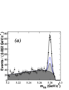
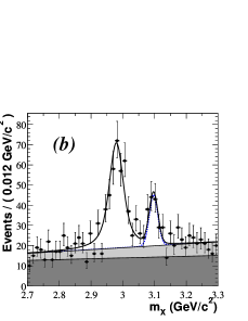
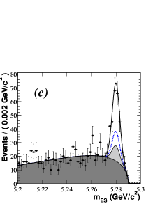
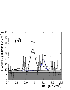
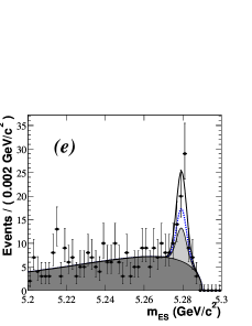
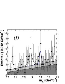
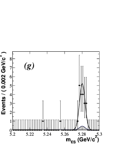
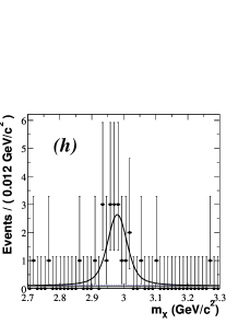
Figure 1: Distributions of $m_{\rm ES}$ (left) and $m_{X}$ (right) for charged $B$ candidates. The $m_{\rm ES}$ distributions displayed here are restricted to the 2.90 $<m_{X}<$ 3.15 ${\mathrm{\,Ge\kern-1.00006ptV\!/}c^{2}}$ range; similarly, the $m_{X}$ distributions include only events in the $m_{\rm ES}$ signal region ($\mbox{$m_{\rm ES}$}>$ 5.27 ${\mathrm{\,Ge\kern-1.00006ptV\!/}c^{2}}$). Each pair corresponds to a different $\eta_{c}$ decay mode: (a, b) $\eta_{c}\rightarrow K^{0}_{\scriptscriptstyle S}K^{\pm}\pi^{\mp}$; (c,d) $\eta_{c}\rightarrow K^{+}\kern-1.60004ptK^{-}\pi^{0}$; (e,f) $\eta_{c}\rightarrow 2(K^{+}\kern-1.60004ptK^{-})$; and (g,h) $\eta_{c}\rightarrow\phi\phi$. The fitted p.d.f. projections are shown as solid curves. In each plot, the dark grey region corresponds to the combinatorial background component, light grey highlights the peaking background, and the dotted line is the sum of the total background and of the ${J\mskip-3.0mu/\mskip-2.0mu\psi\mskip 2.0mu}$ component.

In the largest samples ($\eta_{c}\rightarrow K^{0}_{\scriptscriptstyle S}K^{\pm}\pi^{\mp}$) we can determine the $\eta_{c}$ width $\Gamma(\eta_{c})$ from a simultaneous fit to neutral and charged $B$ data. We find $\Gamma(\eta_{c})$ = 39.7 $\pm$ 6.6 ${\mathrm{\,Me\kern-1.00006ptV\!/}c^{2}}$, where the error is statistical only, consistent with the BABAR measurement, $\Gamma(\eta_{c})$ = 34.3 $\pm$ 2.3 $\pm$ 0.9 ${\mathrm{\,Me\kern-1.00006ptV\!/}c^{2}}$ gamma .

The systematic uncertainty associated with the fitted signal yield includes three components: the uncertainty in the fixed parameters, the uncertainty associated with the Dalitz weighting procedure, and the uncertainty associated with the p.d.f. models. The first component is evaluated by varying each fixed parameter, one at a time, by one standard deviation and repeating the fit. This component is dominated by the uncertainty on $\Gamma(\eta_{c})$ (0–3% fractional uncertainty in $\cal B$, depending on the mode). For the second component, the fit is repeated without applying the Dalitz-correction procedure; half of the difference on the $\eta_{c}$ signal yield (0–2% in $\cal B$) is conservatively assigned as the corresponding systematic uncertainty. The last component is dominated by the uncertainty in the peaking background model. This error is evaluated by varying the assumed $m_{X}$ dependence from a first- to a second-order polynomial; it typically amounts to 4%, and exceeds 10% only for the $\eta_{c}\rightarrow 2(K^{+}\kern-1.60004ptK^{-})$ modes. The error associated with the $m_{X}$ resolution function model (0–5%) is estimated by using, instead of a single Gaussian function fitted to the data, double-Gaussian resolution functions fitted to each simulated signal sample.

Efficiencies are computed with simulated signal events that are reconstructed and selected using the same procedure as for the data, including the yield-extraction fit.

Table 2: Efficiencies and relative systematic uncertainties.

		$B^{+}\rightarrow\eta_{c}K^{+}$					$B^{0}\rightarrow\eta_{c}K^{0}_{\scriptscriptstyle S}$
		$K^{0}_{\scriptscriptstyle S}K^{\pm}\pi^{\mp}$	$K^{+}\kern-1.60004ptK^{-}\pi^{0}$	$2(K^{+}\kern-1.60004ptK^{-})$	$\phi\phi$		$K^{0}_{\scriptscriptstyle S}K^{\pm}\pi^{\mp}$	$K^{+}\kern-1.60004ptK^{-}\pi^{0}$	$2(K^{+}\kern-1.60004ptK^{-})$	$\phi\phi$
		Signal efficiency
		0.213	0.124	0.155	0.194		0.184	0.126	0.147	0.170
Source of uncertainty		Relative uncertainty on signal efficiency(%)
Monte Carlo statistics		1.0	1.5	1.2	1.1		1.2	1.3	1.2	1.1
Tracking		6.0	3.4	6.0	6.0		7.8	5.2	7.8	7.8
$K^{0}_{\scriptscriptstyle S}$ reconstruction		3.0	-	-	-		6.0	3.0	3.0	3.0
Particle identification		3.9	6.5	12.1	8.0		1.5	3.9	9.4	5.9
$\pi^{0}$ reconstruction		-	5.0	-	-		-	5.0	-	-
Selection cuts		2.7	2.8	1.7	2.2		3.3	3.5	3.1	3.4
Yield-extraction fit		3.0	3.0	3.0	3.0		3.0	3.0	3.0	3.0
Total uncertainty		8.8	9.8	13.9	10.7		10.9	9.9	13.3	11.2

We apply small corrections, determined from data, to the efficiency calculation to account for the overestimation of the tracking and particle-identification performance, and of the $\pi^{0}$ and $K^{0}_{\scriptscriptstyle S}$ reconstruction efficiencies. A systematic uncertainty is assigned to each correction to account for the limited size and purity of the control sample used in computing that correction. For example, for the fast kaon identification, we correct the simulation using a pure sample of $D^{*+}\rightarrow\pi^{+}D^{0}$ decays with $D^{0}\rightarrow K^{-}\pi^{+}$. We include in the particle-identification systematic uncertainty contributions associated with the sample size, the background subtraction, and the different kinematics of this decay chain compared to the two-body $B^{+}\rightarrow\eta_{c}K^{+}$ decay. Similarly, corrections affecting the $\pi^{0}$ reconstruction are calibrated using real and simulated $e^{+}e^{-}\rightarrow\tau^{+}\tau^{-}$ and multihadron samples.

In addition, after all corrections, we compare our signal simulation to appropriate control samples with similar kinematics or final-state topology, in order to quantify the ability of the simulation to model the kinematic and event-shape variables used in the event selection. The small residual differences in the efficiencies at the cut value are assigned as systematic uncertainties affecting the selection procedure.

Finally, we assign a systematic uncertainty to the yield-extraction fit by evaluating the influence of mixing background events with simulated signal events. Values for the efficiencies, the corrections, and the corresponding systematic uncertainties are reported in Table 2.

The results on the products of the branching fractions for each mode are listed in Table 3.

Table 3: Measured branching-fraction products $\cal B$($B\rightarrow\eta_{c}K$)$\times$$\cal B$($\eta_{c}$ $\rightarrow X$) (10^-6). The first error is statistical and the second is the total systematic uncertainty.

$\eta_{c}$ decay channel	$B^{+}\rightarrow\eta_{c}K^{+}$	$B^{0}\rightarrow\eta_{c}K^{0}$
$\eta_{c}\rightarrow K^{0}K^{-}\pi^{+}$	48.6 $\pm$ 3.9 $\pm$ 4.9	42.6 $\pm$ 6.8 $\pm$ 5.2
$\eta_{c}\rightarrow K^{+}\kern-1.60004ptK^{-}\pi^{0}$	12.9 $\pm$ 1.7 $\pm$ 1.6	11.1 $\pm$ 2.6 $\pm$ 1.3
$\eta_{c}\rightarrow 2(K^{+}\kern-1.60004ptK^{-})$	2.0 $\pm$ 0.6 $\pm$ 0.4	0.9 $\pm$ 0.9 $\pm$ 0.4
$\eta_{c}\rightarrow\phi\phi$	4.7 $\pm$ 1.2 $\pm$ 0.5	2.4 $\pm$ 1.4 $\pm$ 0.3

We use the world-average values for the $K^{0}_{\scriptscriptstyle S}\rightarrow\pi^{+}\pi^{-}$, $\pi^{0}\rightarrow\gamma\gamma$ and $\phi\rightarrow K^{+}K^{-}$ branching fractions PDG and include their uncertainties in the systematic error. The systematic error also comprises the uncertainties from the determination of the number of $B\kern 1.79993pt\overline{\kern-1.79993ptB}{}$ pairs (1.1%), from the likelihood fit, and from the signal efficiency. We assume that the branching fraction of the $\mathchar 28935\relax{(4S)}$ into $B\kern 1.79993pt\overline{\kern-1.79993ptB}{}$ is 100%, with an equal admixture of charged and neutral $B$ final states. We do not include any additional uncertainty due to these assumptions. Possible interference effects between the $B\rightarrow\eta_{c}K$ signal and the peaking background are neglected.

The decay amplitudes for $\eta_{c}\rightarrow K^{+}\kern-1.60004ptK^{-}\pi^{0}$ and $\eta_{c}\rightarrow K^{0}K^{-}\pi^{+}$ are related by isospin symmetry. The expected ratio of branching fractions, using the appropriate Clebsch-Gordon coefficients, is 0.25. Our measurements are consistent with this value for both the $B^{+}$ (0.27 $\pm$ 0.04 $\pm$ 0.03) and the $B^{0}$ (0.26 $\pm$ 0.07 $\pm$ 0.03) sample. We therefore combine our results for these modes and use the world average for the $\eta_{c}\rightarrow K\kern 1.99997pt\overline{\kern-1.99997ptK}{}\pi$ branching fraction (0.055 $\pm$ 0.017 PDG ) to derive

$${\cal B}(B^{+}\rightarrow\eta_{c}K^{+})=(1.34\pm 0.09\pm 0.13\pm 0.41)\times 10^{-3}$$

$${\cal B}(B^{0}\rightarrow\eta_{c}K^{0})=(1.18\pm 0.16\pm 0.13\pm 0.37)\times 10^{-3}$$

where the first error is statistical, the second systematic, and the third due to the uncertainty on the $\eta_{c}\rightarrow K\kern 1.99997pt\overline{\kern-1.99997ptK}{}\pi$ branching fraction. In the combination we separate correlated and uncorrelated uncertainties to weight the individual results and obtain the total systematic error. We also compute the ratio of neutral over charged $B$ decays ${\cal B}(B^{0}\rightarrow\eta_{c}K^{0})/{\cal B}(B^{+}\rightarrow\eta_{c}K^{+})=0.87\pm 0.13\pm 0.07$, and, multiplying by the mean lifetime ratio $\tau_{B^{+}}/\tau_{B^{0}}=1.085\pm 0.017$ PDG , we derive the ratio of partial widths

$$\Gamma(B^{0}\rightarrow\eta_{c}K^{0})/\Gamma(B^{+}\rightarrow\eta_{c}K^{+})=0.94\pm 0.14\pm 0.08.$$

To determine $R_{K}=\Gamma(B\rightarrow\eta_{c}K)/\Gamma(B\rightarrow{J\mskip-3.0mu/\mskip-2.0mu\psi\mskip 2.0mu}K)$, we use the BABAR measurements ExclBabar of the branching fractions, $\cal B$($B^{+}\rightarrow{J\mskip-3.0mu/\mskip-2.0mu\psi\mskip 2.0mu}K^{+}$) = $(10.1\pm 0.3\pm 0.5)\times 10^{-4}$ and $\cal B$($B^{0}\rightarrow{J\mskip-3.0mu/\mskip-2.0mu\psi\mskip 2.0mu}K^{0}$) = $(8.5\pm 0.5\pm 0.6)\times 10^{-4}$. We obtain

$$R_{K}(B^{+})=1.33\pm 0.10\pm 0.12\pm 0.41$$

$$R_{K}(B^{0})=1.39\pm 0.20\pm 0.13\pm 0.43,$$

where the first error is statistical, the second systematic, and the third due to $\eta_{c}\rightarrow K\kern 1.99997pt\overline{\kern-1.99997ptK}{}\pi$ branching fraction. Our results agree with most predictions for $R_{K}$, which range from 0.9 to 2.3 QCD ; RK1 ; RK2 ; RK3 ; RK4 .

The measured values of $\cal B$($\eta_{c}\rightarrow 2(K^{+}\kern-1.60004ptK^{-})$) and $\cal B$($\eta_{c}\rightarrow\phi\phi$) have higher uncertainties and therefore these modes are not used for averages. We can express our $\eta_{c}\rightarrow 2(K^{+}\kern-1.60004ptK^{-})$ and $\eta_{c}\rightarrow\phi\phi$ results in terms of ratios to the best-measured branching fractions of $\eta_{c}\rightarrow K\kern 1.99997pt\overline{\kern-1.99997ptK}{}\pi$, thereby cancelling all fully-correlated systematic uncertainties. We average results on charged $B$ decays and neutral $B$ decays, taking into account correlations in the systematic uncertainties, to obtain ${\cal B}(\eta_{c}\rightarrow 2(K^{+}\kern-1.60004ptK^{-}))/{\cal B}(\eta_{c}\rightarrow K\kern 1.99997pt\overline{\kern-1.99997ptK}{}\pi)=(2.3\pm 0.7\pm 0.6)\times 10^{-2}$ and ${\cal B}(\eta_{c}\rightarrow\phi\phi)/{\cal B}(\eta_{c}\rightarrow K\kern 1.99997pt\overline{\kern-1.99997ptK}{}\pi)=(5.5\pm 1.4\pm 0.5)\times 10^{-2}$. These results can be translated into $\eta_{c}$ branching fractions:

$${\cal B}(\eta_{c}\rightarrow 2(K^{+}\kern-1.60004ptK^{-}))=(1.3\pm 0.4\pm 0.3\pm 0.4)\times 10^{-3}$$

$${\cal B}(\eta_{c}\rightarrow\phi\phi)=(3.0\pm 0.8\pm 0.3\pm 0.9)\times 10^{-3},$$

where the third error is due to the uncertainty of $\cal B$($\eta_{c}\rightarrow K\kern 1.99997pt\overline{\kern-1.99997ptK}{}\pi$). Note that about half of the $\eta_{c}\rightarrow 2(K^{+}\kern-1.60004ptK^{-})$ events are due to $\eta_{c}\rightarrow\phi\phi$, $\phi\rightarrow K^{+}K^{-}$ decays. Our measured branching fractions for $\eta_{c}\rightarrow 2(K^{+}\kern-1.60004ptK^{-})$ and $\eta_{c}\rightarrow\phi\phi$ are consistent with recent results from Belle and BES 4kBelle ; 2phiBES and are smaller than those of earlier experiments PDG .

As a cross-check, we can extract the branching fraction of ${J\mskip-3.0mu/\mskip-2.0mu\psi\mskip 2.0mu}$ decaying into the $2(K^{+}\kern-1.60004ptK^{-})$ final state from the measured number of ${J\mskip-3.0mu/\mskip-2.0mu\psi\mskip 2.0mu}$ events in the appropriate $B^{+}$ and $B^{0}$ samples. Assuming the same efficiencies as for the $B\rightarrow\eta_{c}K$ ($\eta_{c}\rightarrow 2(K^{+}\kern-1.60004ptK^{-})$) processes and using the BABAR measurements of $\cal B$($B^{+}\rightarrow{J\mskip-3.0mu/\mskip-2.0mu\psi\mskip 2.0mu}K^{+}$) and of $\cal B$($B^{0}\rightarrow{J\mskip-3.0mu/\mskip-2.0mu\psi\mskip 2.0mu}K^{0}$) ExclBabar , we obtain ${\cal B}(J/\psi\rightarrow 2(K^{+}\kern-1.60004ptK^{-}))=(1.0\pm 0.5)\times~{}10^{-3}~{}~{}(B^{+})$ and ${\cal B}(J/\psi\rightarrow 2(K^{+}\kern-1.60004ptK^{-}))=(0.1\pm 0.2)\times~{}10^{-3}~{}~{}(B^{0})$, where the error is statistical only. These results are consistent with the world average, ${\cal B}(J/\psi\rightarrow 2(K^{+}\kern-1.60004ptK^{-}))$= (0.7 $\pm$ 0.3 ) $\times$ 10^-3 PDG .

In summary, we have studied $B\rightarrow\eta_{c}K$ decays with $\eta_{c}$ decaying into $K^{0}_{\scriptscriptstyle S}K^{\pm}\pi^{\mp}$, $K^{+}\kern-1.60004ptK^{-}\pi^{0}$, $2(K^{+}\kern-1.60004ptK^{-})$, and $\phi\phi$. Using the first two decay channels, we have measured the branching fractions ${\cal B}(B^{+}\rightarrow\eta_{c}K^{+})=(1.34\pm 0.09\pm 0.13\pm 0.41)\times 10^{-3}$ and ${\cal B}(B^{0}\rightarrow\eta_{c}K^{0})=(1.18\pm 0.16\pm 0.13\pm 0.37)\times 10^{-3}$, which improve the statistical precision of, and are in good agreement with, previous measurements EtacCLEO ; EtacBelle . We have also measured the branching-fraction ratios ${\cal B}(\eta_{c}\rightarrow 2(K^{+}\kern-1.60004ptK^{-}))/{\cal B}(\eta_{c}\rightarrow K\kern 1.99997pt\overline{\kern-1.99997ptK}{}\pi)=(2.3\pm 0.7\pm 0.6)\times 10^{-2}$ and ${\cal B}(\eta_{c}\rightarrow\phi\phi)/{\cal B}(\eta_{c}\rightarrow K\kern 1.99997pt\overline{\kern-1.99997ptK}{}\pi)=(5.5\pm 1.4\pm 0.5)\times 10^{-2}$, where $\eta_{c}\rightarrow 2(K^{+}\kern-1.60004ptK^{-})$ includes $\eta_{c}\rightarrow\phi\phi$ events with $\phi\rightarrow K^{+}K^{-}$. The inferred branching fractions of $\eta_{c}\rightarrow 2(K^{+}\kern-1.60004ptK^{-})$ and $\eta_{c}\rightarrow\phi\phi$ are in good agreement with recent results and smaller than suggested by earlier experiments.

We are grateful for the excellent luminosity and machine conditions provided by our PEP-II colleagues, and for the substantial dedicated effort from the computing organizations that support BABAR. The collaborating institutions wish to thank SLAC for its support and kind hospitality. This work is supported by DOE and NSF (USA), NSERC (Canada), IHEP (China), CEA and CNRS-IN2P3 (France), BMBF and DFG (Germany), INFN (Italy), FOM (The Netherlands), NFR (Norway), MIST (Russia), and PPARC (United Kingdom). Individuals have received support from the A. P. Sloan Foundation, Research Corporation, and Alexander von Humboldt Foundation.

References

(1)BABAR Collaboration, B. Aubert et al., Phys. Rev. Lett. 89, 201802 (2002).
(2) Belle Collaboration, K. Abe et al., Phys. Rev. D 66, 071102 (2002).
(3) N. G. Deshpande and J. Trampetic, Phys. Lett. B 339, 270 (1994).
(4) M. R. Ahmady and R. R. Mendel, Z. Phys. C 65, 263 (1995).
(5) P. Colangelo, C. A. Domingues, and N. Paver, Phys. Lett. B 352, 134 (1995).
(6) M. Gourdin, Y. Y. Keum, and X.-Y. Pham, Phys. Rev. D 52, 1597 (1995).
(7) D. S. Hwang and G.-H. Kim, Z. Phys. C 76, 107 (1997).
(8) Charge conjugate modes are implicity included throughout this paper.
(9)BABAR Collaboration, B. Aubert et al., Nucl. Instr. Meth. A 479, 1 (2002).
(10) Particle Data Group, K. Hagiwara et al., Phys. Rev. D 66, 010001 (2002)
and 2003 off-year partial update for the 2004 edition available on the PDG WWW pages
(URL: http://pdg.lbl.gov/).
(11) CLEO Collaboration, D. M. Asner et al., Phys. Rev. D 53, 1039 (1996).
(12) ARGUS Collaboration, H. Albrecht et al., Z. Phys. C 48, 543 (1990).
(13)BABAR Collaboration, B. Aubert et al., hep-ex/0311038, submitted to Phys. Rev. Lett. .
(14)BABAR Collaboration, B. Aubert et al., Phys. Rev. D 65, 032001 (2002).
(15) Belle Collaboration, H.-C. Huang et al., Phys. Rev. Lett. 91, 241802 (2003).
(16) BES Collaboration, J. Z. Bai et al., Phys. Lett. B 578, 16 (2004).
(17) CLEO Collaboration, K. W. Edwards et al., Phys. Rev. Lett. 86, 30 (2001).
(18) Belle Collaboration, F. Fang et al., Phys. Rev. Lett. 90, 071801 (2003).