Limits on the Decay-Rate Difference of Neutral-$B$ Mesons and on $C\!P$, $T$, and $C\!PT$ Violation in $B^{0}{\kern-2.30405pt\kern 2.59189pt\overline{\kern-2.59189ptB}{}^{0}}$ Oscillations
The BABAR Collaboration

Abstract

Using events in which one of two neutral-$B$ mesons from the decay of an $\mathchar 28935\relax{(4S)}$ resonance is fully reconstructed, we set limits on the difference between the decay rates of the two neutral-$B$ mass eigenstates and on $C\!P$, $T$, and $C\!PT$ violation in $B^{0}{\kern-1.60004pt\kern 1.79993pt\overline{\kern-1.79993ptB}{}^{0}}$ mixing. The reconstructed decays, comprising both $C\!P$ and flavor eigenstates, are obtained from 88 million $\mathchar 28935\relax{(4S)}\rightarrow B\kern 1.79993pt\overline{\kern-1.79993ptB}{}$ decays collected with the BABAR detector at the PEP-II asymmetric-energy $B$ Factory at SLAC. We determine six independent parameters governing oscillations ($\Delta m$, $\Delta\Gamma/\Gamma$), $C\!PT$ and $C\!P$ violation ($\mathop{\rm Re}{\mathsf{z}}$, $\mathop{\rm Im}{\mathsf{z}}$), and $C\!P$ and $T$ violation ($\mathop{\rm Im}\lambda_{C\!P}$, $|q/p|$), where $\lambda_{C\!P}$ characterizes $B^{0}$ and $\kern 1.79993pt\overline{\kern-1.79993ptB}{}^{0}$ decays to states of charmonium plus $K^{0}_{\scriptscriptstyle S}$ or $K^{0}_{\scriptscriptstyle L}$. The results are

$$\begin{array}[]{ r@{\ \ =\ }r@{.}l@{\pm 0.}l@{{\rm(stat.)}\pm 0.} l@{{\rm{(syst.)}}\ \ [}r@{,\ }l@{]}l}\mathop{\rm{sgn}}(\mathop{\rm Re}\lambda_{C\!P})\Delta\Gamma/\Gamma&-0&008&037&018&-0.084&0.068&~{},\\ |q/p|&1&029&013&011&1.001&1.057&~{},\\ \left(\mathop{\rm Re}\lambda_{C\!P}/|\lambda_{C\!P}|\right)\mathop{\rm Re}{\mathsf{z}}&0&014&035&034&-0.072&0.101&~{},\\ \mathop{\rm Im}{\mathsf{z}}&0&038&029&025&-0.028&0.104&~{}.\end{array}$$

The values inside square brackets indicate the 90% confidence-level intervals. The values of $\mathop{\rm Im}\lambda_{C\!P}$ and $\Delta m$ are consistent with previous analyses and are used as cross-checks. These measurements are in agreement with Standard Model expectations.

I Introduction and analysis overview

The mass difference $\Delta m$ between the $B^{0}$ mass eigenstates has been measured with high precision at $B$-factory experiments ref:dM-babar-had ; ref:dM-babar-dstlnu ; ref:dM-babar-dilep ; ref:dM-belle , and $C\!P$ violation has been observed in neutral-$B$-meson decays to states like ${J\mskip-3.0mu/\mskip-2.0mu\psi\mskip 2.0mu}K^{0}_{\scriptscriptstyle S}$ ref:sin2b-babar ; ref:sin2b-belle . However, our knowledge of other aspects of neutral-$B$-meson oscillations is meager. In this paper, we provide direct limits on the total decay-rate difference $\Delta\Gamma$ between the $B^{0}$ mass eigenstates, and on $C\!P$, $T$, and $C\!PT$ violation due to oscillations alone.

In the Standard Model, the ratio $\Delta\Gamma/\Delta m$ is of order $m_{b}^{2}/m_{t}^{2}$ and thus quite small. Recent calculations of $\Delta\Gamma/\Gamma$, including $1/m_{b}$ contributions and part of the next-to-leading order QCD corrections ref:dighe ; ref:ciuchini , find values in the approximate range $-0.2\%$ to $-0.3\%$. Existing limits for $|\Delta\Gamma/\Gamma|$ ref:cleochid ; ref:delphi are relatively weak ($\sim 20\%$). The large data sets available at asymmetric-energy $B$ factories provide an opportunity to look for deviations from the Standard Model.

The $C\!P$-violating asymmetry observed in neutral-$B$-meson decays to states like ${J\mskip-3.0mu/\mskip-2.0mu\psi\mskip 2.0mu}K^{0}_{\scriptscriptstyle S}$ is due to the interference between decay amplitudes to a $C\!P$ eigenstate with and without mixing. $C\!P$ violation in mixing alone leads to different rates for the transitions $B^{0}$ $\rightarrow$ $\kern 1.79993pt\overline{\kern-1.79993ptB}{}^{0}$ and $\kern 1.79993pt\overline{\kern-1.79993ptB}{}^{0}$ $\rightarrow$ $B^{0}$. This can be measured, for example, by comparing the decay rates to $\ell^{-}\ell^{-}X$ and $\ell^{+}\ell^{+}X$ from semileptonic decays of pairs of neutral-$B$ mesons arising from the $\mathchar 28935\relax{(4S)}$ ref:babardileptonTviolation . The only semileptonic decays generated by first-order weak interactions are $B^{0}\rightarrow\ell^{+}\nu X$ and $\kern 1.79993pt\overline{\kern-1.79993ptB}{}^{0}\rightarrow\ell^{-}\overline{\nu}\overline{X}$ and the $C\!P$ invariance of strong and electromagnetic interactions guarantees that these have equal rates. As a result, any asymmetry in the dilepton rates can be ascribed to $C\!P$ violation in mixing. While $C\!P$ violation in mixing is suppressed in the Standard Model ref:ciuchini ; ref:absqopSM ; ref:beneke , additional virtual contributions from new physics could obviate this suppression. Similarly, new physics may introduce additional intrinsic $T$ violation or even $C\!PT$ violation in mixing. It is these possibilities for the breaking of discrete symmetries in mixing itself that we address in this analysis using nonleptonic decays that are completely reconstructed.

The behavior of neutral-$B$ mesons is sensitive to $C\!PT$ violation ref:sanda ; ref:ko ; ref:bbCPT . A theorem ref:cpttheo founded on general principles of relativistic quantum field theory states that the $C\!PT$ symmetry holds for any local field theory satisfying Lorentz invariance. The $C\!PT$ symmetry is the only combination of $C$, $P$, and $T$ that is not known to be violated. Nevertheless, it is possible that $C\!PT$ symmetry could fail at short distances ref:cptbreak . Strict constraints on $C\!PT$ violation have been obtained in the neutral-kaon system ref:cptkaons . Limits in the $B$-meson system have been obtained previously ref:otherCPTBtests ; ref:dM-belle .

To measure $\Delta\Gamma$ and $C\!P$, $T$, or $C\!PT$ violation, we observe the time dependence of decays of neutral-$B$ mesons produced in pairs at the $\mathchar 28935\relax{(4S)}$ resonance. The usual approach to mixing and $C\!P$ analyses ref:dM-babar-had ; ref:dM-babar-dstlnu ; ref:dM-babar-dilep ; ref:dM-belle ; ref:sin2b-babar ; ref:sin2b-belle allows for exponential decay, modulated by oscillatory terms with frequency $\Delta m$. These analyses neglect the difference $\Delta\Gamma$ between the decay rates of the two mass eigenstates, which would introduce terms with a new time dependence ${\exp(\pm\Delta\Gamma t/2)}$. Violation of $C\!P$, $T$, or $C\!PT$  in the mixing of the neutral-$B$ mesons would modify the coefficients of the various terms involving exponential and oscillatory behavior. To detect these potential subtle changes requires precision measurements of the decays, detailed consideration of systematic effects, and thorough treatment of coherent production of neutral-$B$-meson pairs from the $\mathchar 28935\relax(4S)$.

This analysis is based on a total of about 88 million $\mathchar 28935\relax{(4S)}\rightarrow B\kern 1.79993pt\overline{\kern-1.79993ptB}{}$ decays collected with the BABAR detector at the PEP-II asymmetric-energy $B$ Factory at the Stanford Linear Accelerator Center. There, 9.0-$\mathrm{\,Ge\kern-1.00006ptV}$ electrons and 3.1-$\mathrm{\,Ge\kern-1.00006ptV}$ positrons annihilate to produce the $B\kern 1.79993pt\overline{\kern-1.79993ptB}{}$ pairs moving along the $e^{-}$ beam direction ($z$-axis) with a Lorentz boost of $\beta\gamma\approx 0.55$. This boost makes it possible to measure the proper-time difference $\Delta t$ between the two $B$ decays. We fully reconstruct one meson from its decay to a flavor eigenstate ($B_{\rm flav}$) or to a $C\!P$ eigenstate ($B_{C\!P}$) composed of charmonium and either a $K^{0}_{\scriptscriptstyle S}$ or $K^{0}_{\scriptscriptstyle L}$. We denote the flavor and $C\!P$ eigenstates jointly by $B_{\rm rec}$. The remaining charged particles in the event, which originate from the other $B$ meson ($B_{\rm tag}$), are used to identify (“tag”) its flavor as $B^{0}$ or $\kern 1.79993pt\overline{\kern-1.79993ptB}{}^{0}$. Not all events can be tagged, but the untagged events are also used in the analysis. The time difference $\Delta t\equiv t_{\rm rec}-t_{\rm tag}\approx\Delta z/(\beta\gamma c)$ is determined from the separation $\Delta z$ along the boost direction of the decay vertices for the fully reconstructed $B$ candidate and the tagging $B$.

A maximum-likelihood fit to the time distributions of tagged and untagged, flavor and $C\!P$ eigenstates determines six independent parameters (see Sec. II) governing oscillations ($\Delta m$, $\Delta\Gamma/\Gamma$), $C\!PT$ and $C\!P$ violation ($\mathop{\rm Re}{\mathsf{z}}$, $\mathop{\rm Im}{\mathsf{z}}$), and $C\!P$ and $T$ violation ($\mathop{\rm Im}\lambda_{C\!P}$, $|q/p|$), where $\lambda_{C\!P}$ is the usual variable used to characterize the decays of neutral-$B$ mesons into final states of charmonium and a $K^{0}_{\scriptscriptstyle S}$ or $K^{0}_{\scriptscriptstyle L}$. The values of $\mathop{\rm Im}\lambda_{C\!P}$ and $\Delta m$ are used as cross-checks with the earlier BABAR $\sin 2\beta$ result ref:sin2b-babar , obtained with the same dataset, and with previous $B$-factory measurements of $\Delta m$ ref:dM-babar-had ; ref:dM-babar-dstlnu ; ref:dM-babar-dilep ; ref:dM-belle . All the parameters are explicitly defined in Sec. II.

The analysis presents several challenges. First, the resolution for $\Delta t$ is comparable to the $B$ lifetime and is asymmetric in $\Delta t$. This asymmetry must be well understood lest it be mistaken for a fundamental asymmetry we seek to measure. Second, tagging assigns flavor incorrectly some fraction of the time. Third, interference between weak decays favored by the Cabibbo-Kobayashi-Maskawa (CKM) quark-mixing matrix and those doubly-Cabibbo-suppressed ($\rm DCS$) cannot be neglected. Fourth, direct $C\!P$ violation in the $B_{C\!P}$ sample could mimic $C\!P$ violation in mixing and must be parameterized appropriately. Finally, we have to account for possible asymmetries induced by the differing response of the detector to positively and negatively charged particles. In resolving all of the above issues we rely mainly on data.

This paper provides a detailed description of the analysis published in Ref. ref:CPTprl , and is organized as follows. In Sec. II we present a general formulation of the time-dependent decay rates of $B^{0}{\kern-1.60004pt\kern 1.79993pt\overline{\kern-1.79993ptB}{}^{0}}$ pairs produced at the $\mathchar 28935\relax{(4S)}$ resonance, including effects from the decay-rate difference, possible $C\!P$ and $C\!PT$ violation in mixing, and interference effects induced by $\rm DCS$ decays. We derive the expressions for $B$ decays to flavor and $C\!P$ eigenstates. In Sec. III we describe the BABAR detector. After discussing the data sample in Sec. IV, we describe the $B$-flavor tagging algorithm in Sec. V. Sec. VI is devoted to the description of the measurement of ${\rm\Delta}z$ and to the determination of $\Delta t$ and its resolution function. In Sec. VII we describe our log-likelihood function and the assumptions made in the fit. The results of the fit are given in Sec. VIII. Cross-checks are discussed in Sec. IX and systematic uncertainties are presented in Sec. X. The results of the analysis are summarized and discussed in Sec. XI.

II General time-dependent decay rates from $\mathchar 28935\relax(4S)\rightarrow B^{0}{\kern-1.60004pt\kern 1.79993pt\overline{\kern-1.79993ptB}{}^{0}}$

The neutral-$B$-meson system can be described by the effective Hamiltonian ${\bf H}={\bf M}-i{\bf\Gamma}/2$, where ${\bf M}$ and ${\bf\Gamma}$ are two-by-two Hermitian matrices describing, respectively, the mass and decay-rate components. $C\!P$ or $C\!PT$ symmetry imposes that $M_{11}=M_{22}$ and $\Gamma_{11}=\Gamma_{22}$, the index $1$ indicating $B^{0}$  and $2$ indicating $\kern 1.79993pt\overline{\kern-1.79993ptB}{}^{0}$. In the limit of $C\!P$ or $T$ invariance, $\Gamma_{12}/M_{12}=\Gamma_{21}/M_{21}=\Gamma_{12}^{*}/M_{12}^{*}$, so $\Gamma_{12}/M_{12}$ is real. These conditions do not depend on the phase conventions chosen for the $B^{0}$ and $\kern 1.79993pt\overline{\kern-1.79993ptB}{}^{0}$. The masses $m_{H,L}$ and decay rates $\Gamma_{H,L}$ of the two eigenstates of ${\bf H}$ form the complex eigenvalues $\omega_{H,L}$

$$\omega_{H,L}\equiv m_{H,L}-\frac{i}{2}\Gamma_{H,L}=m-\frac{i}{2}\Gamma\pm\sqrt{\left(M_{12}-\frac{i}{2}\Gamma_{12}\right)\left(M_{12}^{*}-\frac{i}{2}\Gamma_{12}^{*}\right)+\frac{1}{4}\left(\delta m-\frac{i}{2}\delta\Gamma\right)^{2}}~{},$$ (1)

where the real part of the square root is taken to be positive and where we define

$$m\equiv\frac{1}{2}(M_{11}+M_{22}) \Gamma\equiv\frac{1}{2}(\Gamma_{11}+\Gamma_{22})~{},$$ ,

$$\delta m\equiv M_{11}-M_{22}\quad \delta\Gamma\equiv\Gamma_{11}-\Gamma_{22}~{}.$$ , (2)

Assuming $C\!PT$ invariance ($\delta m=0,\delta\Gamma=0$), and anticipating that $|\Delta\Gamma|\ll\Delta m$, we have

$$\Delta m \equiv m_{H}-m_{L}\approx 2|M_{12}|~{},$$

$$\Delta\Gamma \equiv \Gamma_{H}-\Gamma_{L}\approx 2|M_{12}|\mathop{\rm Re}(\Gamma_{12}/M_{12})~{}.$$ (3)

Here we have taken $\Delta m$ to be the mass of the heavier eigenstate minus the mass of the lighter one. Thus, $\Delta\Gamma$ is the decay rate of the heavier state minus the decay rate of the lighter one and its sign is not known a priori.

With $C\!PT$ symmetry, the light and heavy mass eigenstates of the neutral-$B$-meson system can be written

$$|B_{L}\rangle = p|B^{0}\rangle+q|\kern 1.79993pt\overline{\kern-1.79993ptB}{}^{0}\rangle~{},$$

$$|B_{H}\rangle = p|B^{0}\rangle-q|\kern 1.79993pt\overline{\kern-1.79993ptB}{}^{0}\rangle~{},$$ (4)

where

$${q\over p}\equiv-\sqrt{{M^{\ast}_{12}-\frac{i}{2}\,\Gamma^{\ast}_{12}\over M_{12}-\frac{i}{2}\,\Gamma_{12}}}~{}.$$ (5)

The magnitude of $q/p$ is very nearly unity:

$$\left|\frac{q}{p}\right|^{2}\approx 1-\mathop{\rm Im}\frac{\Gamma_{12}}{M_{12}}~{}.$$ (6)

In the Standard Model, the $C\!P$- and $T$-violating quantity $|q/p|^{2}-1$ is small not just because $|\Gamma_{12}|$ is small, but additionally because the $C\!P$-violating quantity $\mathop{\rm Im}(\Gamma_{12}/M_{12})$ is suppressed by an additional factor $(m_{c}^{2}-m_{u}^{2})/m_{b}^{2}\approx 0.1$ relative to $|\Gamma_{12}/M_{12}|$. Violation of $C\!P$ is not possible if two of the quark masses (for quarks of the same charge) are identical, for then we could redefine two new quark states with equal masses so that one of them did not mix with the two remaining states. The mixing among two generations would be inadequate to support $C\!P$ violation. When the remaining Standard Model factors are included, the expectation is $|\mathop{\rm Im}({\Gamma_{12}}/{M_{12}})|<10^{-3}$ ref:ciuchini ; ref:absqopSM ; ref:beneke .

$C\!PT$ violation in mixing can be described conveniently by the phase-convention–independent quantity

$${\mathsf{z}} \equiv {\delta m-\frac{i}{2}\,\delta\Gamma\over 2\sqrt{\left(M_{12}-\frac{i}{2}\,\Gamma_{12}\right)\left(M^{\ast}_{12}-\frac{i}{2}\,\Gamma^{\ast}_{12}\right)+\frac{1}{4}\left(\delta m-\frac{i}{2}\,\delta\Gamma\right)^{2}}}$$ (7)

$${=} \frac{\delta m-\frac{i}{2}\,\delta\Gamma}{\Delta m-\frac{i}{2}\Delta\Gamma}~{}.$$

The generalization of the eigenstates in Eq. (4) when we account for $C\!PT$ violation can be written

$$|B_{L}\rangle = p\sqrt{1-{\mathsf{z}}}|B^{0}\rangle+q\sqrt{1+{\mathsf{z}}}|\kern 1.79993pt\overline{\kern-1.79993ptB}{}^{0}\rangle~{},$$

$$|B_{H}\rangle = p\sqrt{1+{\mathsf{z}}}|B^{0}\rangle-q\sqrt{1-{\mathsf{z}}}|\kern 1.79993pt\overline{\kern-1.79993ptB}{}^{0}\rangle~{},$$ (8)

where we maintain the definition of $q/p$ given in Eq. (5). The result, when time evolution is included, is that states that begin as purely $B^{0}$ or $\kern 1.79993pt\overline{\kern-1.79993ptB}{}^{0}$ after a time $t$ will be mixtures

$$|{{B^{0}}_{\text{phys}}(t)}\rangle = \bigl{[}g_{+}(t)+{\mathsf{z}}g_{-}(t)\bigr{]}\,|{B^{0}}\rangle$$ (9)

$$-\sqrt{1-{\mathsf{z}}^{2}}\frac{q}{p}\,g_{-}(t)\,|{\kern 1.79993pt\overline{\kern-1.79993ptB}{}^{0}}\rangle~{},$$

$$|{{\kern 1.79993pt\overline{\kern-1.79993ptB}{}^{0}}_{\text{phys}}(t)}\rangle = \bigl{[}g_{+}(t)-{\mathsf{z}}g_{-}(t)\bigr{]}\,|{\kern 1.79993pt\overline{\kern-1.79993ptB}{}^{0}}\rangle$$ (10)

$$-\sqrt{1-{\mathsf{z}}^{2}}\frac{p}{q}\,g_{-}(t)\,|{B^{0}}\rangle~{},$$

where we have introduced

$$g_{\pm}(t)=\frac{1}{2}(e^{-i\omega_{H}t}\pm e^{-i\omega_{L}t})~{}.$$ (11)

Invariance under $C\!P$ or under $T$ requires that

$$|\langle B^{0}|{{\kern 1.79993pt\overline{\kern-1.79993ptB}{}^{0}}_{\text{phys}}(t)}\rangle|=|\langle\kern 1.79993pt\overline{\kern-1.79993ptB}{}^{0}|{{B^{0}}_{\text{phys}}(t)}\rangle|~{};$$ (12)

i.e., $|q/p|=1$, which is guaranteed by $\mathop{\rm Im}(\Gamma_{12}/M_{12})=0$. Table 1 shows the constraints on $|q/p|$ and ${\mathsf{z}}$ for the different possible symmetry scenarios. The Standard Model corresponds to the second configuration ($C\!PT$ symmetry, with $C\!P$ and $T$ violated). Note that two of these scenarios are degenerate. With $C\!P$ symmetry in $B^{0}{\kern-1.60004pt\kern 1.79993pt\overline{\kern-1.79993ptB}{}^{0}}$ oscillations, this experiment cannot distinguish between $T$ and $C\!PT$ both being conserved or violated.

Table 1: Constraints on $|q/p|$ and ${\mathsf{z}}$ due to $C\!P$, $T$, and $C\!PT$ symmetries in $B^{0}{\kern-1.60004pt\kern 1.79993pt\overline{\kern-1.79993ptB}{}^{0}}$ oscillations.

		$C\!PT$
		$C\!P$, $T$	,	, $T$	$C\!P$,	,
$|q/p|$		$=1$	$\neq 1$	$=1$	$=1$	$\neq 1$
${\mathsf{z}}$		$=0$	$=0$	$\neq 0$	$=0$	$\neq 0$

II.1 Effects of Coherence

At the $\mathchar 28935\relax(4S)$ resonance, neutral-$B$ mesons are produced in coherent p-wave pairs. If we subsequently observe one $B$-meson decay to the state $f_{1}$ at time $t_{0}=0$ and the other decay to the state $f_{2}$ at some later time $t$, we cannot in general know whether $f_{1}$ came from the decay of a $B^{0}$ or a $\kern 1.79993pt\overline{\kern-1.79993ptB}{}^{0}$, and similarly for the state $f_{2}$. If $A_{1,2}$ and ${\overline{A}}_{1,2}$ are the amplitudes for the decay of $B^{0}$ and $\kern 1.79993pt\overline{\kern-1.79993ptB}{}^{0}$, respectively, to the states $f_{1}$ and $f_{2}$, then the overall amplitude is given by

$${\cal A} = a_{+}g_{+}(t)+a_{-}g_{-}(t)~{},$$ (13)

where

$$a_{+} = -A_{1}{\overline{A}}_{2}+{\overline{A}}_{1}A_{2}~{},$$

$$a_{-} = \sqrt{1-{\mathsf{z}}^{2}}\left[{p\over q}A_{1}A_{2}-{q\over p}{\overline{A}}_{1}{\overline{A}}_{2}\right]+{\mathsf{z}}\left[A_{1}{\overline{A}}_{2}+{\overline{A}}_{1}A_{2}\right]~{}.$$

Using the relations

$$|g_{\pm}(t)|^{2}=\frac{1}{2}\,e^{-\Gamma t}\left[\cosh(\Delta\Gamma t/2)\pm\cos(\Delta mt)\right]$$ (15)

and

$$g_{+}^{\ast}(t)\,g_{-}(t)=-\frac{1}{2}\,e^{-\Gamma t}\left[\sinh(\Delta\Gamma t/2)+i\,\sin(\Delta mt)\right]~{},$$ (16)

we find the decay rate

$${{\rm d}N\over{\rm d}t} \propto e^{-\Gamma|t|}\Biggl{\{}{1\over 2}c_{+}\cosh(\Delta\Gamma t/2)+{1\over 2}c_{-}\cos(\Delta mt)$$ (17)

$$\qquad-\mathop{\rm Re}s\,\sinh(\Delta\Gamma t/2)+\mathop{\rm Im}s\,\sin(\Delta mt)\Biggr{\}}~{},~{}~{}~{}~{}~{}~{}$$

where

$$c_{\pm}=|a_{+}|^{2}\pm|a_{-}|^{2}~{},\quad s=a_{+}^{*}a_{-}~{}.$$ (18)

The absolute value in the leading exponential in Eq. (17) is introduced for later convenience.

Now let us take $f_{1}\equiv f_{{\rm tag}}$ to be the state that is incompletely reconstructed and that provides the tagging decay, and $f_{2}\equiv f_{{\rm rec}}$ to be the fully reconstructed state (flavor or $C\!P$ eigenstate). Then we have $t=t_{{\rm rec}}-t_{{\rm tag}}$ and Eq. (II.1) becomes

$$a_{+} = -A_{{\rm tag}}{\overline{A}}_{\rm rec}+{\overline{A}}_{{\rm tag}}A_{\rm rec}~{},$$

$$a_{-} = \sqrt{1-{\mathsf{z}}^{2}}\left[{p\over q}A_{{\rm tag}}A_{\rm rec}-{q\over p}{\overline{A}}_{{\rm tag}}{\overline{A}}_{\rm rec}\right]$$ (19)

$$+{\mathsf{z}}\left[A_{{\rm tag}}{\overline{A}}_{\rm rec}+{\overline{A}}_{{\rm tag}}A_{\rm rec}\right]~{}.$$

If instead the tagged decay occurs second, we would need to redefine $t$, $a_{+}$ and $a_{-}$ by interchanging the labels “tag” and “rec”. This would amount to the replacements $t\rightarrow-t$, $a_{+}\rightarrow-a_{+}$, and $a_{-}\rightarrow a_{-}$. However, we see that Eq. (17) is actually unaffected by these changes and that we can instead retain the definitions $t=t_{{\rm rec}}-t_{{\rm tag}}$ and those of Eq. (19). Thus, Eqs. (17)-(19) apply independent of the order of the decays of the tagged and fully reconstructed $B$ mesons.

A fully reconstructed flavor state cannot always be unambiguously associated with either $B^{0}$ or $\kern 1.79993pt\overline{\kern-1.79993ptB}{}^{0}$. $\rm DCS$ decays, such as $B^{0}\rightarrow D^{+}\pi^{-}$, occur at a rate suppressed by roughly $|V_{ub}^{*}V_{cd}/V_{cb}^{*}V_{ud}|^{2}\approx(0.02)^{2}$. Although this can be neglected, interference between favored and suppressed amplitudes is reduced by only a factor of approximately $0.02$ ref:owenandus , and must be taken into account.

Tagging cannot be done perfectly, largely because the tagging state is incompletely reconstructed. We account for this by measuring the wrong-tag probability from the data. However, even if our tagging were perfect in principle, it would be afflicted with the same complication from $\rm DCS$ decays as the fully reconstructed state. The full expressions for the real coefficients $c_{\pm}$ and the complex coefficient $s$, containing the $\rm DCS$ amplitudes, are

$$c_{\pm} = \biggl{\{}\left|\overline{A}_{{\rm rec}}A_{{\rm tag}}-A_{{\rm rec}}\overline{A}_{{\rm tag}}\right|^{2}\pm|{\mathsf{z}}|^{2}\left|\overline{A}_{{\rm rec}}A_{{\rm tag}}+A_{{\rm rec}}\overline{A}_{{\rm tag}}\right|^{2}\pm|1-{\mathsf{z}}^{2}|\,\left|\frac{p}{q}A_{{\rm rec}}A_{{\rm tag}}-\frac{q}{p}\overline{A}_{{\rm rec}}\overline{A}_{{\rm tag}}\right|^{2}$$ (20)

$$\quad\pm 2{\rm Re}\left[{\mathsf{z}}^{\ast}\sqrt{1-{\mathsf{z}}^{2}}\,\left(\frac{p}{q}A_{{\rm rec}}A_{{\rm tag}}-\frac{q}{p}\overline{A}_{{\rm rec}}\overline{A}_{{\rm tag}}\right)\left(\overline{A}_{{\rm rec}}A_{{\rm tag}}+A_{{\rm rec}}\overline{A}_{{\rm tag}}\right)^{\ast}\right]\biggr{\}}$$

$$s = \biggl{\{}\left(A_{{\rm rec}}\overline{A}_{{\rm tag}}-\overline{A}_{{\rm rec}}A_{{\rm tag}}\right)^{\ast}\left[\sqrt{1-{\mathsf{z}}^{2}}\left(\frac{p}{q}A_{{\rm rec}}A_{{\rm tag}}-\frac{q}{p}\overline{A}_{{\rm rec}}\overline{A}_{{\rm tag}}\right)+{\mathsf{z}}\left(\overline{A}_{{\rm rec}}A_{{\rm tag}}+A_{{\rm rec}}\overline{A}_{{\rm tag}}\right)\right]\biggr{\}}~{}.$$ (21)

Table 2: The coefficient $c_{+}$ from Eq. (20), evaluated to leading order in the small quantities ${\mathsf{z}}$, $\lambda_{{Bf}}$, $\lambda_{Bt}$, $\overline{\lambda}_{{\kern 1.25995pt\overline{\kern-1.25995ptB}{}f}}$, and $\overline{\lambda}_{{\kern 1.25995pt\overline{\kern-1.25995ptB}{}t}}$. If the tagging state for a $B^{0}$ tag is $f_{Bt}$, then the tagging state for a $\kern 1.79993pt\overline{\kern-1.79993ptB}{}^{0}$ is the $C\!P$-conjugate state, $f_{{\kern 1.25995pt\overline{\kern-1.25995ptB}{}t}}$, and similarly for the fully reconstructed states. The decay amplitudes are $A_{Bt}=\langle f_{{Bt}}|{\cal H}|B^{0}\rangle$, ${\overline{A}}_{{Bt}}=\langle f_{{Bt}}|{\cal H}|\kern 1.79993pt\overline{\kern-1.79993ptB}{}^{0}\rangle$, $A_{{\kern 1.25995pt\overline{\kern-1.25995ptB}{}t}}=\langle f_{{\kern 1.25995pt\overline{\kern-1.25995ptB}{}t}}|{\cal H}|B^{0}\rangle$, ${\overline{A}}_{{\kern 1.25995pt\overline{\kern-1.25995ptB}{}t}}=\langle f_{{\kern 1.25995pt\overline{\kern-1.25995ptB}{}t}}|{\cal H}|\kern 1.79993pt\overline{\kern-1.79993ptB}{}^{0}\rangle$, and similarly for ${\rm rec}={Bf},{\kern 1.79993pt\overline{\kern-1.79993ptB}{}f},C\!P$.

$B_{\rm tag}$	$B_{\rm rec}$	$c_{+}$
$B^{0}$	$B^{0}$	$|A_{Bt}|^{2}|A_{{Bf}}|^{2}\,|p/q|^{2}$
$B^{0}$	$\kern 1.79993pt\overline{\kern-1.79993ptB}{}^{0}$	$|A_{Bt}|^{2}|\overline{A}_{{\kern 1.25995pt\overline{\kern-1.25995ptB}{}f}}|^{2}$
$\kern 1.79993pt\overline{\kern-1.79993ptB}{}^{0}$	$B^{0}$	$|\overline{A}_{{\kern 1.25995pt\overline{\kern-1.25995ptB}{}t}}|^{2}|A_{{Bf}}|^{2}$
$\kern 1.79993pt\overline{\kern-1.79993ptB}{}^{0}$	$\kern 1.79993pt\overline{\kern-1.79993ptB}{}^{0}$	$|\overline{A}_{{\kern 1.25995pt\overline{\kern-1.25995ptB}{}t}}|^{2}|\overline{A}_{{\kern 1.25995pt\overline{\kern-1.25995ptB}{}f}}|^{2}\,|q/p|^{2}$
$B^{0}$	$B_{C\!P}$	$|A_{Bt}|^{2}|A_{C\!P}|^{2}\,|p/q|^{2}[1+|\lambda_{C\!P}|^{2}-4\mathop{\rm Re}\lambda_{C\!P}\mathop{\rm Re}\lambda_{Bt}+2\mathop{\rm Re}{\mathsf{z}}\mathop{\rm Re}\lambda_{C\!P}-2\mathop{\rm Im}{\mathsf{z}}\mathop{\rm Im}\lambda_{C\!P}]$
$\kern 1.79993pt\overline{\kern-1.79993ptB}{}^{0}$	$B_{C\!P}$	$|\overline{A}_{{\kern 1.25995pt\overline{\kern-1.25995ptB}{}t}}|^{2}|A_{C\!P}|^{2}\,[1+|\lambda_{C\!P}|^{2}-4\mathop{\rm Re}\lambda_{C\!P}\mathop{\rm Re}\overline{\lambda}_{{\kern 1.25995pt\overline{\kern-1.25995ptB}{}t}}-2\mathop{\rm Re}{\mathsf{z}}\mathop{\rm Re}\lambda_{C\!P}-2\mathop{\rm Im}{\mathsf{z}}\mathop{\rm Im}\lambda_{C\!P}]$

Table 3: The coefficient $c_{-}$ from Eq. (20), evaluated to leading order in the small quantities ${\mathsf{z}}$, $\lambda_{{Bf}}$, $\lambda_{Bt}$, $\overline{\lambda}_{{\kern 1.25995pt\overline{\kern-1.25995ptB}{}f}}$, and $\overline{\lambda}_{{\kern 1.25995pt\overline{\kern-1.25995ptB}{}t}}$. See caption of Table 2 for the definition of the various quantities.

$B_{\rm tag}$	$B_{\rm rec}$	$c_{-}$
$B^{0}$	$B^{0}$	$-|A_{Bt}|^{2}|A_{{Bf}}|^{2}\,|p/q|^{2}$
$B^{0}$	$\kern 1.79993pt\overline{\kern-1.79993ptB}{}^{0}$	$|A_{Bt}|^{2}|\overline{A}_{{\kern 1.25995pt\overline{\kern-1.25995ptB}{}f}}|^{2}$
$\kern 1.79993pt\overline{\kern-1.79993ptB}{}^{0}$	$B^{0}$	$|\overline{A}_{{\kern 1.25995pt\overline{\kern-1.25995ptB}{}t}}|^{2}|A_{{Bf}}|^{2}$
$\kern 1.79993pt\overline{\kern-1.79993ptB}{}^{0}$	$\kern 1.79993pt\overline{\kern-1.79993ptB}{}^{0}$	$-|\overline{A}_{{\kern 1.25995pt\overline{\kern-1.25995ptB}{}t}}|^{2}|\overline{A}_{{\kern 1.25995pt\overline{\kern-1.25995ptB}{}f}}|^{2}\,|q/p|^{2}$
$B^{0}$	$B_{C\!P}$	$|A_{Bt}|^{2}|A_{C\!P}|^{2}\,|p/q|^{2}[-1+|\lambda_{C\!P}|^{2}-4\mathop{\rm Im}\lambda_{C\!P}\mathop{\rm Im}\lambda_{Bt}-2\mathop{\rm Re}{\mathsf{z}}\mathop{\rm Re}\lambda_{C\!P}+2\mathop{\rm Im}{\mathsf{z}}\mathop{\rm Im}\lambda_{C\!P}]$
$\kern 1.79993pt\overline{\kern-1.79993ptB}{}^{0}$	$B_{C\!P}$	$|\overline{A}_{{\kern 1.25995pt\overline{\kern-1.25995ptB}{}t}}|^{2}|A_{C\!P}|^{2}\,[1-|\lambda_{C\!P}|^{2}+4\mathop{\rm Im}\lambda_{C\!P}\mathop{\rm Im}\overline{\lambda}_{{\kern 1.25995pt\overline{\kern-1.25995ptB}{}t}}+2\mathop{\rm Re}{\mathsf{z}}\mathop{\rm Re}\lambda_{C\!P}+2\mathop{\rm Im}{\mathsf{z}}\mathop{\rm Im}\lambda_{C\!P}]$

Table 4: The complex coefficient $s$ from Eq. (21), evaluated to leading order in the small quantities ${\mathsf{z}}$, $\lambda_{{Bf}}$, $\lambda_{Bt}$, $\overline{\lambda}_{{\kern 1.25995pt\overline{\kern-1.25995ptB}{}f}}$, and $\overline{\lambda}_{{\kern 1.25995pt\overline{\kern-1.25995ptB}{}t}}$. See caption of Table 2 for the definition of the various quantities.

$B_{\rm tag}$	$B_{\rm rec}$	$s$
$B^{0}$	$B^{0}$	$|A_{Bt}|^{2}|A_{{Bf}}|^{2}\,|p/q|^{2}[\lambda_{Bt}^{*}-\lambda_{{Bf}}^{*}]$
$B^{0}$	$\kern 1.79993pt\overline{\kern-1.79993ptB}{}^{0}$	$|A_{Bt}|^{2}|\overline{A}_{{\kern 1.25995pt\overline{\kern-1.25995ptB}{}f}}|^{2}[\lambda_{Bt}-\overline{\lambda}_{{\kern 1.25995pt\overline{\kern-1.25995ptB}{}f}}-{\mathsf{z}}]$
$\kern 1.79993pt\overline{\kern-1.79993ptB}{}^{0}$	$B^{0}$	$|\overline{A}_{{\kern 1.25995pt\overline{\kern-1.25995ptB}{}t}}|^{2}|A_{{Bf}}|^{2}[\overline{\lambda}_{{\kern 1.25995pt\overline{\kern-1.25995ptB}{}t}}-\lambda_{{Bf}}+{\mathsf{z}}]$
$\kern 1.79993pt\overline{\kern-1.79993ptB}{}^{0}$	$\kern 1.79993pt\overline{\kern-1.79993ptB}{}^{0}$	$|\overline{A}_{{\kern 1.25995pt\overline{\kern-1.25995ptB}{}t}}|^{2}|\overline{A}_{{\kern 1.25995pt\overline{\kern-1.25995ptB}{}f}}|^{2}\,|q/p|^{2}[\overline{\lambda}_{{\kern 1.25995pt\overline{\kern-1.25995ptB}{}t}}^{*}-\overline{\lambda}_{{\kern 1.25995pt\overline{\kern-1.25995ptB}{}f}}^{*}]$
$B^{0}$	$B_{C\!P}$	$|A_{Bt}|^{2}|A_{C\!P}|^{2}\,|p/q|^{2}[|\lambda_{C\!P}|^{2}\lambda_{Bt}-\lambda_{C\!P}^{*}+\lambda_{Bt}^{*}-|\lambda_{C\!P}|^{2}{\mathsf{z}}]$
$\kern 1.79993pt\overline{\kern-1.79993ptB}{}^{0}$	$B_{C\!P}$	$|\overline{A}_{{\kern 1.25995pt\overline{\kern-1.25995ptB}{}t}}|^{2}|A_{C\!P}|^{2}\,[\overline{\lambda}_{{\kern 1.25995pt\overline{\kern-1.25995ptB}{}t}}-\lambda_{C\!P}+|\lambda_{C\!P}|^{2}\overline{\lambda}_{{\kern 1.25995pt\overline{\kern-1.25995ptB}{}t}}^{*}+{\mathsf{z}}]$

Terms proportional to $A_{{\rm rec}}$$\overline{A}_{{\rm tag}}$ and $\overline{A}_{{\rm rec}}$$A_{{\rm tag}}$ are associated with decays with no net oscillation between the two neutral-$B$ decays, while terms proportional to ($q/p$)$\overline{A}_{{\rm rec}}$$\overline{A}_{{\rm tag}}$ and ($p/q$)$A_{{\rm rec}}$$A_{{\rm tag}}$ represent a net oscillation.

We characterize each final state $f$ through the parameter

$$\lambda_{{f}}=\frac{q}{p}\frac{\overline{A}_{f}}{A_{f}}~{},$$ (22)

where $f$ can be “rec”(which can be itself “flav” or “$C\!P$”) or “tag”. In the absence of $\rm DCS$ decays, $\lambda_{{\rm flav}}$ (i.e., $\lambda_{{\rm rec}}$ when the reconstructed state is a flavor eigenstate, not a $C\!P$ eigenstate) and $\lambda_{{\rm tag}}$ would be either zero or infinite. With a contribution from $\rm DCS$ decays they are non-zero and finite.

If the reconstructed flavor state $f_{{\rm flav}}$ is ostensibly a $B^{0}$ (hereafter indicated as ${Bf}$ to avoid ambiguities with the tag state) then $|\lambda_{{\rm rec}}|\equiv|\lambda_{{Bf}}|\ll 1$. Conversely, if the reconstructed state appears to come from a $\kern 1.79993pt\overline{\kern-1.79993ptB}{}^{0}$ (indicated as ${\kern 1.79993pt\overline{\kern-1.79993ptB}{}f}$), then $|\lambda_{{\kern 1.25995pt\overline{\kern-1.25995ptB}{}f}}|\gg 1$, and it is convenient to introduce $\overline{\lambda}_{{\kern 1.25995pt\overline{\kern-1.25995ptB}{}f}}\equiv 1/\lambda_{{\kern 1.25995pt\overline{\kern-1.25995ptB}{}f}}$. The pattern for the tagging state (“tag”$=Bt,{\kern 1.79993pt\overline{\kern-1.79993ptB}{}t}$) is similar. If the reconstructed state is a $C\!P$ eigenstate, then $|\lambda_{{\rm rec}}|\equiv|\lambda_{C\!P}|$ is of order unity.

In practice, terms quadratic in ${\mathsf{z}}$ or in a small $\lambda_{f}$ are not important. The expressions for $c_{\pm}$ and $s$ when only linear terms in small quantities are retained are shown in Tables 2,  3, and 4. The analysis uses the full expressions, without simplification.

It is appropriate to assume that the decays to flavor eigenstates we consider are dominated by a single weak mechanism: $b\rightarrow c\overline{u}d$. While we can find a mechanism for $\overline{b}\rightarrow c\overline{u}d$ (which is a $\rm DCS$ process), there are no alternative first-order weak processes that produce $c\overline{u}d$ from a $b$ quark. Then even if there are several contributions to the decay, each possibly with its own strong phase, the $C\!P$-conjugate decay differs only by changing a single common weak phase so that $|A_{{Bf}}|=|{\overline{A}}_{{\kern 1.25995pt\overline{\kern-1.25995ptB}{}f}}|$, $|{\overline{A}}_{{Bf}}|=|{A}_{{\kern 1.25995pt\overline{\kern-1.25995ptB}{}f}}|$ (and similarly for tagging states). In fact, even if this assumption is not rigorously true, any violation will be absorbed in tagging and reconstruction efficiencies, which are determined from the data, as described in Sec. VII. These equalities relate the four permutations that arise from the tag and reconstructed state being either $B^{0}$ or $\kern 1.79993pt\overline{\kern-1.79993ptB}{}^{0}$.

II.2 Ensembles of States

In principle, every hadronic final state $f_{{h}}$ has a different $\lambda_{h}$,which can be written as $\lambda_{h}=|\lambda_{h}|e^{-i\phi_{h}^{\mathrm{even}}}e^{-i\phi_{h}^{\mathrm{odd}}}$, where $\phi_{h}^{\mathrm{even}}$ and $\phi_{h}^{\mathrm{odd}}$ are strong ($C\!P$-even) and weak ($C\!P$-odd) phases that arise from the ratio of the amplitudes of the $B^{0}$ and $\kern 1.79993pt\overline{\kern-1.79993ptB}{}^{0}$ decays to $f_{{h}}$. Assuming that there is a single weak phase involved, the $C\!P$-conjugate state $\overline{f}_{{h}}$ will have ${\overline{\lambda}}_{\overline{h}}=|p/q|^{2}|\lambda_{h}|e^{-i\phi_{h}^{\mathrm{even}}}e^{i\phi_{h}^{\mathrm{odd}}}$.

If we sum squares of amplitudes over a collection $F$ of flavor states that are ostensibly $B^{0}$, the terms that do and do not contain $\lambda_{{\rm flav}}$ are of the form

$$\sum_{f_{{h}}\in F}|A_{h}|^{2}\lambda_{h}\qquad{\rm and}\qquad\sum_{f_{{h}}\in F}|A_{h}|^{2}~{},$$ (23)

so we can define an effective $\lambda_{{Bf}}$ by

$$\lambda_{{{Bf}}}=\frac{\sum_{f_{{h}}\in F}|A_{h}|^{2}\lambda_{h}}{\sum_{f_{{h}}\in F}|A_{h}|^{2}}~{}.$$ (24)

Similarly, for flavor states that are ostensibly $\kern 1.79993pt\overline{\kern-1.79993ptB}{}^{0}$,

$${\overline{\lambda}}_{{\kern 1.25995pt\overline{\kern-1.25995ptB}{}f}}=\frac{\sum_{\overline{f}_{{h}}\in F}|\overline{A}_{\overline{h}}|^{2}{\overline{\lambda}}_{\overline{h}}}{\sum_{\overline{f}_{{h}}\in F}|\overline{A}_{\overline{h}}|^{2}}~{}.$$ (25)

The two complex numbers $\lambda_{{Bf}}$ and ${\overline{\lambda}}_{{\kern 1.25995pt\overline{\kern-1.25995ptB}{}f}}$ encapsulate the effects due to $\rm DCS$ decays in the fully reconstructed $B$ decay, as long as the terms quadratic in $\lambda_{h}$ and $\overline{\lambda}_{\overline{h}}$, suppressed by roughly $|V_{ub}^{*}V_{cd}/V_{cb}^{*}V_{ud}|^{2}\approx(0.02)^{2}$, are omitted.

The same argument applies to tagging states. If the collection of states contributing to a $B^{0}$ or $\kern 1.79993pt\overline{\kern-1.79993ptB}{}^{0}$ tag is $\alpha$ then

$$\lambda_{{Bt}} = \frac{\sum_{f_{{h}}\in\alpha}|A_{h}|^{2}\lambda_{h}}{\sum_{f_{{h}}\in\alpha}|A_{h}|^{2}}~{},$$ (26)

$${\overline{\lambda}}_{{\kern 1.25995pt\overline{\kern-1.25995ptB}{}t}} = \frac{\sum_{\overline{f}_{{h}}\in\alpha}|\overline{A}_{\overline{h}}|^{2}\overline{\lambda}_{\overline{h}}}{\sum_{\overline{f}_{{h}}\in\alpha}|\overline{A}_{\overline{h}}|^{2}}~{}.$$ (27)

In practice, we do not use separate $\lambda_{{\rm tag}}$ parameters for each tagging category $\alpha$ (i.e., each collection of states of similar character, as described in Sec. V), but simply one for $B^{0}$ and one for $\kern 1.79993pt\overline{\kern-1.79993ptB}{}^{0}$, setting aside the lepton tag category, which is free of $\rm DCS$ decays. This treatment is flexible enough to incorporate the $\rm DCS$-decay effects that can mimic the asymmetries we seek in the analysis.

Henceforth, expressions like $\lambda_{{\rm flav}}$ and $\lambda_{{\rm tag}}$ refer to an appropriate sum over observed states. The summation over states $f_{{h}}$ in a tagging category should be thought of as extending over those states that are reconstructed as belonging to the given category. In this way, we incorporate implicitly the tagging efficiency of each state $f_{{h}}$. The reconstruction efficiency is incorporated in an analogous fashion into $\lambda_{{\rm flav}}$.

Data from directly related $C\!P$ final states like ${J\mskip-3.0mu/\mskip-2.0mu\psi\mskip 2.0mu}K^{0}_{\scriptscriptstyle S}$, with $\eta_{C\!P}=-1$, and ${J\mskip-3.0mu/\mskip-2.0mu\psi\mskip 2.0mu}K^{0}_{\scriptscriptstyle L}$, with $\eta_{C\!P}=+1$, where $\eta_{C\!P}$ is the $C\!P$ eigenvalue of the final state, can be combined by assuming that their time distributions are identical, except for the factor $\eta_{C\!P}$. We use a single parameter $\lambda_{C\!P}$ obtained multiplying Eq. (22) by $\eta_{C\!P}$. We assume $r_{C\!P}=|\overline{A}_{C\!P}/A_{C\!P}|=1$ as expected theoretically at the $10^{-3}$ level ref:grossman and as supported experimentally by:

1. the average of $B$-factory measurements of states of charmonium and $K^{0}_{\scriptscriptstyle S}$ or $K^{0}_{\scriptscriptstyle L}$, from which it has been obtained $r_{C\!P}=0.949\pm 0.045$ ref:sin2b-babar ; ref:sin2b-belle , when $\Delta\Gamma$, $|q/p|-1$ and ${\mathsf{z}}$ are assumed to be zero;

2. the average of CLEO and BABAR measurements of the $C\!P$ asymmetry in the charged mode $B^{\pm}\rightarrow{J\mskip-3.0mu/\mskip-2.0mu\psi\mskip 2.0mu}K^{\pm}$, from which it is found $r_{C\!P,{J\mskip-3.0mu/\mskip-2.0mu\psi\mskip 2.0mu}K^{\pm}}=1.008\pm 0.025$ ref:cleojpsikp ; ref:babarjpsikp , combined with isospin symmetry to relate with the $C\!P$ final states ref:theojpsikp .

II.3 Sensitivity of Distributions to Parameters

From Eq. (17) and Tables 2, 3, and 4, it can be seen that while $\mathop{\rm Im}\lambda_{C\!P}$, $\mathop{\rm Im}{\mathsf{z}}$, $|q/p|$, and $r_{C\!P}$ are unambiguously determined, $\mathop{\rm Re}{\mathsf{z}}$ appears only in the product $\mathop{\rm Re}\lambda_{C\!P}$$\mathop{\rm Re}{\mathsf{z}}$ or else is suppressed by the small factor $\Delta\Gamma/\Gamma$. Similarly, the sign of $\Delta\Gamma$ cannot be determined separately from the sign of $\mathop{\rm Re}\lambda_{C\!P}$ since $\Delta\Gamma$ always appears multiplied by $\mathop{\rm Re}\lambda_{C\!P}$ in its dominant contribution. Its value is known only through $\mathop{\rm Re}\lambda_{C\!P}=\pm\sqrt{|\lambda_{C\!P}|^{2}-(\mathop{\rm Im}\lambda_{C\!P})^{2}}$, where the choice of sign could be made by a separate measurement that directly determines the sign of $\mathop{\rm Re}\lambda_{C\!P}$. As a result, the parameters that can be determined by this analysis are $\mathop{\rm{sgn}}(\mathop{\rm Re}\lambda_{C\!P})\Delta\Gamma/\Gamma$, $|q/p|$, $\left(\mathop{\rm Re}\lambda_{C\!P}/|\lambda_{C\!P}|\right)\mathop{\rm Re}{\mathsf{z}}$, $\mathop{\rm Im}{\mathsf{z}}$, $\mathop{\rm Im}\lambda_{C\!P}/|\lambda_{C\!P}|$, $r_{C\!P}$, $\Delta m$, and $\Gamma$. In practice, we fix $r_{C\!P}$ and $\Gamma$ in the nominal fit, and vary them for systematic studies.

Data for final states that are $C\!P$ eigenstates and those that are flavor eigenstates are both needed for the analysis, as shown in Table 5. The sensitivity to $\left(\mathop{\rm Re}\lambda_{C\!P}/|\lambda_{C\!P}|\right)\mathop{\rm Re}{\mathsf{z}}$ and $\mathop{\rm Im}\lambda_{C\!P}/|\lambda_{C\!P}|$ is provided by the decays to $C\!P$ eigenstates $B_{C\!P}$, for which the accompanying $t$ dependence is even for the former and odd for the latter. The $B_{\rm flav}$ sample contributes marginally to these parameters because it lacks explicit dependence on $\mathop{\rm Im}\lambda_{C\!P}/|\lambda_{C\!P}|$ and the dependence on $\mathop{\rm Re}{\mathsf{z}}$ is scaled by the $\sinh\left(\Delta\Gamma t/2\right)$ term, which is small for small $\Delta\Gamma$.

In contrast, the parameters $|q/p|$ and $\mathop{\rm Im}{\mathsf{z}}$ (and $\Delta m$) are determined by the large $B_{\rm flav}$ sample, where the former is associated with a $t$-even distribution and the latter with a $t$-odd distribution. For small values of $\Delta\Gamma/\Gamma$, the determination of $\Delta\Gamma/\Gamma$ is dominated by the $B_{C\!P}$ sample, despite the smallness of this sample compared to the $B_{\rm flav}$ sample. This is because in the flavor sample the leading dependence on $\Delta\Gamma$ is proportional to $\Delta\Gamma^{2}$, while in the $C\!P$ sample it is proportional to $\Delta\Gamma$. The contribution of $\sinh(\Delta\Gamma t/2)$ is the same for both $B^{0}$ and $\kern 1.79993pt\overline{\kern-1.79993ptB}{}^{0}$ tags, so events that cannot be tagged may be included in the analysis to improve sensitivity. The $B_{C\!P}$ sample is also sensitive to the sign of $\Delta\Gamma/\Gamma$ (up to the sign ambiguity from $\mathop{\rm Re}\lambda_{C\!P}$).

Overall, the combined use of the $B_{\rm flav}$ and $B_{C\!P}$ samples provides sensitivity to the full set of physical parameters, since they are determined either from different samples, or from different $t$ dependences.

Table 5: Dominant dependence of the time distributions on the physical parameters measured with fully reconstructed flavor and $C\!P$ states. Sensitivity is specific to terms in the time dependence that are either $t$-even or $t$-odd. The flavor sample is much larger than the $C\!P$ sample.

	$B_{\rm flav}$		$B_{C\!P}$
Parameter	$t$-even	$t$-odd	$t$-even	$t$-odd
$|q/p|$	$\times$
$\Delta m$	$\times$
$\mathop{\rm Im}{\mathsf{z}}$		$\times$
$\left(\mathop{\rm Re}\lambda_{C\!P}/|\lambda_{C\!P}|\right)\mathop{\rm Re}{\mathsf{z}}$			$\times$
$r_{C\!P}$			$\times$
$\mathop{\rm{sgn}}(\mathop{\rm Re}\lambda_{C\!P})\Delta\Gamma/\Gamma$				$\times$
$\mathop{\rm Im}\lambda_{C\!P}/|\lambda_{C\!P}|$				$\times$

As we show in Tables 2, 3, and 4, if the reconstructed state is a flavor eigenstate, the $\rm DCS$-decay effects in tagging are negligible except in the $\sin(\Delta mt)$ term, for the other terms are suppressed by both a power of $\lambda_{{\rm flav}}$ and a power of $\lambda_{{\rm tag}}$. Conversely, if the reconstructed state is a $C\!P$ eigenstate with $|\lambda_{C\!P}|\approx 1$, the effects from $\rm DCS$ decays are confined to the terms even in $t$.

III The BABAR detector

The BABAR detector is described in detail elsewhere ref:babar-nim , so here we give only a brief description of the apparatus.

Surrounding the beam-pipe is a five-layer silicon vertex tracker (SVT), which gives precisely measured points along the trajectories of charged particles as they leave the interaction region. Outside the SVT is a 40-layer drift chamber (DCH) filled with an 80:20 helium-isobutane gas mixture, chosen to minimize multiple scattering. Charged-particle tracking and the determination of momenta through track curvature rely on the DCH and SVT measurements in the 1.5-T magnetic field generated by a superconducting solenoid. The DCH and SVT measurements of $dE/dx$ energy loss also contribute to charged-particle identification.

Surrounding the drift chamber is a novel detector of internally reflected Cerenkov radiation (DIRC), giving charged-particle identification in the central region of the detector. Outside the DIRC is a highly segmented electromagnetic calorimeter (EMC) composed of CsI(Tl) crystals. The EMC is used to detect photons and neutral hadrons through shower shapes and is also used to identify electrons. Finally, the flux return of the superconducting coil surrounding the EMC is instrumented with resistive plate chambers interspersed with iron for the identification of muons and neutral hadrons (IFR).

A detailed Monte Carlo program based on the GEANT4 ref:geant4 software package is used to simulate the BABAR detector response and performance.

IV Data samples and $B$-meson reconstruction

From a sample of about 88 million $\mathchar 28935\relax{(4S)}\rightarrow B\kern 1.79993pt\overline{\kern-1.79993ptB}{}$ decays, we select events in which one of the $B$ mesons is completely reconstructed in either a neutral or a charged hadronic final state, using the same criteria used for the BABAR $\sin{2\beta}$ measurement ref:sin2b-babar and for measurements of $\Delta m$ using hadronic final states ref:dM-babar-had . Neutral-$B$ mesons are reconstructed in either a flavor ($B_{\rm flav}$) or $C\!P$ ($B_{C\!P}$) eigenstate. The charged-$B$-meson decays are used as control samples in the cross-checks described in Sec. IX.2. The decay modes used for the flavor sample, the $C\!P$ sample, the control samples are displayed in Table 6. Details on charged particle and neutral reconstruction, particle identification and reconstruction of $B$ mesons can be found in Secs. II and III in Ref. ref:babar-stwob-prd .

Table 6: The flavor, $C\!P$, and control sample decay modes used in this analysis. The ${J\mskip-3.0mu/\mskip-2.0mu\psi\mskip 2.0mu}$ is always identified in the $e^{+}e^{-}$ or $\mu^{+}\mu^{-}$ modes. The $a_{1}^{+}$ is reconstructed only in $\pi^{+}\pi^{+}\pi^{-}$. The $K^{0}_{\scriptscriptstyle S}$ is identified in the $\pi^{+}\pi^{-}$ mode, except otherwise specified. All charge-conjugate decay modes are included implicitly.

Samples	Decay modes
$B_{\rm flav}$	$B^{0}\rightarrow D^{*-}\pi^{+}(\rho^{+},a_{1}^{+})$
		$D^{*-}\rightarrow{\overline{D}}^{0}\pi^{-}$
		${\overline{D}}^{0}\rightarrow K^{+}\pi^{-},K^{+}\pi^{-}\pi^{0},$
		$\qquad~{}~{}~{}K^{+}\pi^{-}\pi^{+}\pi^{-},$
		$\qquad~{}~{}~{}K^{0}_{\scriptscriptstyle S}\pi^{+}\pi^{-}$
	$B^{0}\rightarrow D^{-}\pi^{+}(\rho^{+},a_{1}^{+})$
		$D^{-}\rightarrow K^{+}\pi^{-}\pi^{-},K^{0}_{\scriptscriptstyle S}\pi^{-}$
	$B^{0}\rightarrow{J\mskip-3.0mu/\mskip-2.0mu\psi\mskip 2.0mu}K^{*0}$
		$K^{*0}\rightarrow K^{+}\pi^{-}$
$B_{C\!P}$	$B^{0}\rightarrow{J\mskip-3.0mu/\mskip-2.0mu\psi\mskip 2.0mu}K^{0}_{\scriptscriptstyle S}$
		$K^{0}_{\scriptscriptstyle S}\rightarrow\pi^{+}\pi^{-},\pi^{0}\pi^{0}$
	$B^{0}\rightarrow\psi{(2S)}K^{0}_{\scriptscriptstyle S}$
		$\psi{(2S)}\rightarrow e^{+}e^{-},\mu^{+}\mu^{-},$
		$\qquad~{}~{}~{}~{}~{}~{}{J\mskip-3.0mu/\mskip-2.0mu\psi\mskip 2.0mu}\pi^{+}\pi^{-}$
	$B^{0}\rightarrow\chi_{c1}K^{0}_{\scriptscriptstyle S}$
		$\chi_{c1}\rightarrow{J\mskip-3.0mu/\mskip-2.0mu\psi\mskip 2.0mu}\,\gamma$
	$B^{0}\rightarrow{J\mskip-3.0mu/\mskip-2.0mu\psi\mskip 2.0mu}K^{0}_{\scriptscriptstyle L}$
Control	$B^{+}\rightarrow\overline{D}^{(*)0}\pi^{+}$
		$\overline{D}^{*0}\rightarrow\overline{D}^{0}\pi^{0}$
	$B^{+}\rightarrow{J\mskip-3.0mu/\mskip-2.0mu\psi\mskip 2.0mu}K^{+}$
	$B^{+}\rightarrow\psi{(2S)}K^{+}$
	$B^{+}\rightarrow\chi_{c1}K^{+}$
	$B^{+}\rightarrow{J\mskip-3.0mu/\mskip-2.0mu\psi\mskip 2.0mu}K^{*+}$
		$K^{*+}\rightarrow K^{0}_{\scriptscriptstyle S}\pi^{+}$

We select $B_{\rm flav}$ and $B_{C\!P}$ candidates by requiring that the difference $\Delta E$ between their energy and the beam energy in the center-of-mass frame be less than $3\sigma$ from zero, where $\sigma$ is the resolution on $\Delta E$. The $\Delta E$ resolution ranges between 10 and 50 $\mathrm{\,Me\kern-1.00006ptV}$ depending on the decay mode. For $B_{\rm flav}$ modes and $B_{C\!P}$ modes involving $K^{0}_{\scriptscriptstyle S}$ ($B_{{C\!P}K^{0}_{\scriptscriptstyle S}}$), the beam-energy substituted mass must be greater than $5.2{\mathrm{\,Ge\kern-1.00006ptV\!/}c^{2}}$. The beam-energy substituted mass is given by

$$m_{\rm ES}=\sqrt{\frac{(s/2+{\bf p}_{i}\cdot{\bf p}_{B})^{2}}{E_{i}^{2}}-p_{B}^{2}}~{},$$ (28)

where $s$ is the square of the center-of-mass energy, $E_{i}$ and ${\bf p}_{i}$ are the total energy and the three-momentum of the initial state in the laboratory frame, and ${\bf p}_{B}$ is the three-momentum of the $B$ candidate in the same frame. In the case of decays to ${J\mskip-3.0mu/\mskip-2.0mu\psi\mskip 2.0mu}K^{0}_{\scriptscriptstyle L}$ ($B_{{C\!P}K^{0}_{\scriptscriptstyle L}}$), the $K^{0}_{\scriptscriptstyle L}$ direction is measured but its momentum is only inferred by constraining the mass of the ${J\mskip-3.0mu/\mskip-2.0mu\psi\mskip 2.0mu}K^{0}_{\scriptscriptstyle L}$ candidate to the known $B^{0}$ mass. As a consequence, there is only one parameter left to define the signal region, which is taken to be $|\Delta E|<10\mathrm{\,Me\kern-1.00006ptV}$.

Fig. 1 shows the $m_{\rm ES}$ distribution for the $B_{\rm flav}$ and $B_{{C\!P}K^{0}_{\scriptscriptstyle S}}$ samples and the $\Delta E$ distribution for the $B_{{C\!P}K^{0}_{\scriptscriptstyle L}}$ candidates, before the vertex requirements (see Sec. VI). The combinatorial background in the $m_{\rm ES}$ distributions is described by the empirical ARGUS phase-space model ref:argus and the signal by a Gaussian distribution. The combinatorial background consists of random combinations of tracks from continuum and $B\kern 1.79993pt\overline{\kern-1.79993ptB}{}$ sources. The former events are dominantly “prompt”, that is, the observed particles point back to the interaction point, whereas the latter events are dominantly “non-prompt”, with particles pointing back to separated vertices. Charmed particles, either from continuum or from $B$-meson decays, contribute to non-prompt background. A small background due to other $B$ decays (not shown in Fig. 1) also peaks at the $B$ mass. The background in the ${J\mskip-3.0mu/\mskip-2.0mu\psi\mskip 2.0mu}K^{0}_{\scriptscriptstyle L}$ channel receives contributions from other $B$ decays with real ${J\mskip-3.0mu/\mskip-2.0mu\psi\mskip 2.0mu}$ mesons in the final state, and from events with fake ${J\mskip-3.0mu/\mskip-2.0mu\psi\mskip 2.0mu}$ mesons constructed from unassociated leptons or from misidentified particles.

After completely reconstructing one $B$ meson, the rest of the event is analyzed to identify the flavor of the opposite $B$ meson and to reconstruct its decay point, as described in Secs. V and VI.

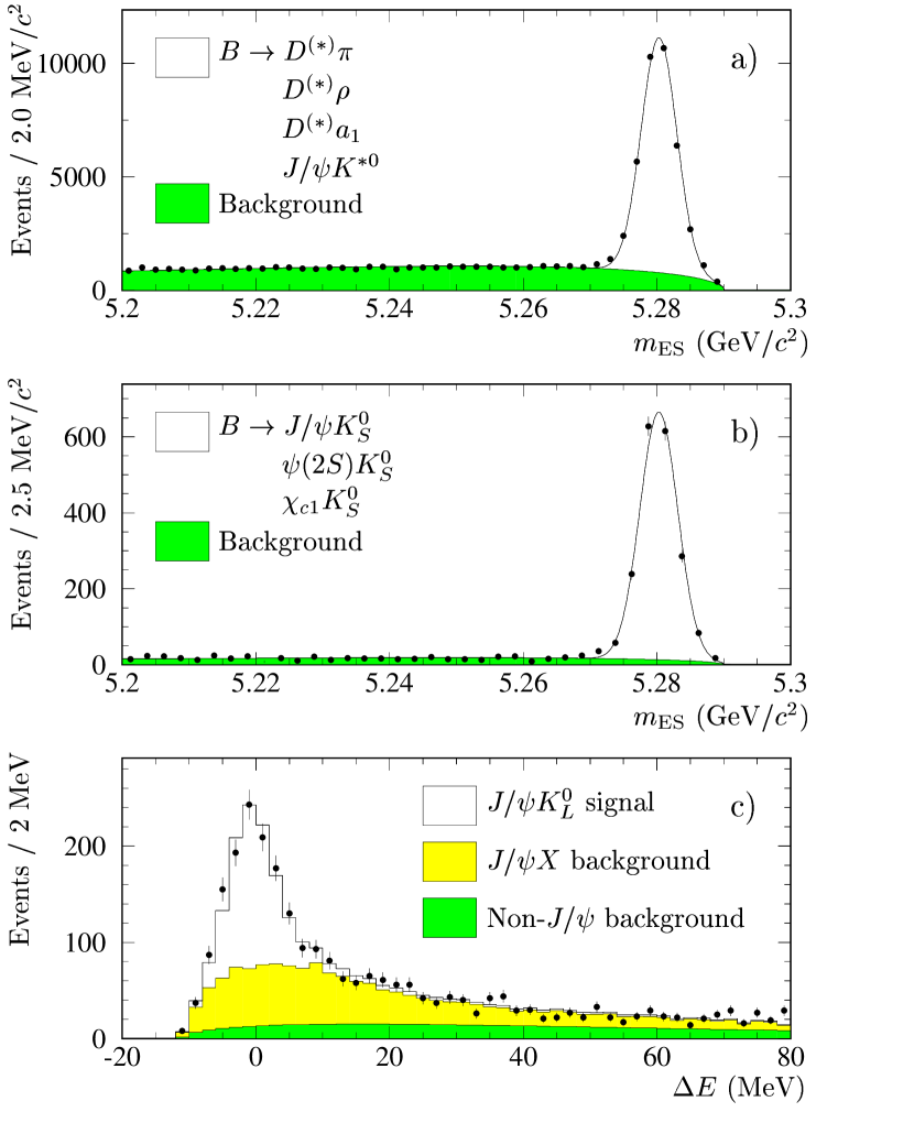
Figure 1: Distributions for $B_{\rm flav}$ and $B_{C\!P}$ candidates before vertex requirements: a) $m_{\rm ES}$ for $B_{\rm flav}$ states; b) $m_{\rm ES}$ for $B^{0}\rightarrow{J\mskip-3.0mu/\mskip-2.0mu\psi\mskip 2.0mu}K^{0}_{\scriptscriptstyle S},\psi{(2S)}K^{0}_{\scriptscriptstyle S},\chi_{c1}K^{0}_{\scriptscriptstyle S}$ final states; and c) $\Delta E$ for the final state $B^{0}\rightarrow{J\mskip-3.0mu/\mskip-2.0mu\psi\mskip 2.0mu}K^{0}_{\scriptscriptstyle L}$. In (a) and (b), the backgrounds are dominantly combinatorial. In (c) there are backgrounds from events containing a true $J/\psi$ but with a spurious $K^{0}_{\scriptscriptstyle L}$. Other background comes from events in which no true $J/\psi$ is present.

Using exactly the same requirements, we analyze GEANT4-simulated samples to check for any biases in the event selection and extracted parameters. The Monte Carlo samples are also used in studies of detector response and to estimate some background sources. The values of the $B$ oscillation and $C\!P$-, $T$-, and $C\!PT$- violating parameters assumed in the simulations are similar to those measured in the data. We use additional samples with significantly different values to check the reliability of the analysis in other regions of the parameter space.

V Flavor tagging

The tracks that are not part of the fully reconstructed $B$ meson are used to determine whether the $B_{\rm tag}$ was a $B^{0}$ or $\kern 1.79993pt\overline{\kern-1.79993ptB}{}^{0}$ when it decayed. This determination cannot be done perfectly. If the probability of an incorrect assignment is $w$, an asymmetry that depends on the difference between $B^{0}$ and $\kern 1.79993pt\overline{\kern-1.79993ptB}{}^{0}$ tags will be reduced by a factor $D=1-2w$, called the dilution. A neural network combining the outputs of algorithms that evaluate the characteristics of each event is used to take into account the correlations between the different sources of flavor information and to estimate $B^{0}$ and $\kern 1.79993pt\overline{\kern-1.79993ptB}{}^{0}$ mistag probabilities for each event. Based on these values and the source of flavor information, the event is tagged and assigned to one of five mutually exclusive tagging categories. The dilution for each category is determined from the data, as described in Sec. VII. Grouping tags into categories, each with a relatively narrow range in mistag probability, increases the overall power of the tagging while simplifying the studies of systematic uncertainties.

Events with an identified primary electron or muon and a kaon with the same charge, if present, are assigned to the Lepton category. Events with both an identified kaon and a low-momentum (soft) pion candidates with opposite charge and similar flight direction are assigned to the KaonI category. Soft pion candidates from $D^{*+}$ decays are selected on the basis of their momentum and direction with respect to the thrust axis of $B_{\rm tag}$. Events with only an identified kaon are assigned to the KaonI or KaonII category depending on the estimated mistag probability. Events with only a soft-pion candidate are assigned to the KaonII category as well. The remaining events are assigned to either the Inclusive or the UnTagged category based on the estimated mistag probability. The UnTagged tagging category has a mistag rate set to 50%, and therefore does not provide tagging information. It does, however, increase the sensitivity to the decay-rate difference $\Delta\Gamma$ and allows the determination from the data of the detector charge asymmetries, as described in Sec. VII. This tagging algorithm is identical to that used in Ref. ref:sin2b-babar .

We consider separate mistag probabilities for $B^{0}$ and $\kern 1.79993pt\overline{\kern-1.79993ptB}{}^{0}$ tags, $w^{\alpha}_{Bt}$ and $w^{\alpha}_{{\kern 1.25995pt\overline{\kern-1.25995ptB}{}t}}$, in each tagging category $\alpha$. From these, we define the average mistag probability $w^{\alpha}=(w^{\alpha}_{Bt}+w^{\alpha}_{{\kern 1.25995pt\overline{\kern-1.25995ptB}{}t}})/2$ and the asymmetry in the mistag rates $\Delta w^{\alpha}=w^{\alpha}_{Bt}-w^{\alpha}_{{\kern 1.25995pt\overline{\kern-1.25995ptB}{}t}}$. A correlation between the average mistag rate and the $\Delta t$ uncertainty $\sigma_{\Delta t}$ estimated event-by-event (discussed in Sec. VI) is observed for kaon-based tags ref:dM-babar-dstlnu ; ref:babar-stwob-prd . For a ${\rm\Delta}t$ uncertainty less than 1.4${\rm\,ps}$, this correlation is found to be approximately linear:

$$w^{\alpha}=w^{\alpha}_{0}+w^{\alpha}_{\rm slope}\sigma_{\Delta t}~{}.$$ (29)

All signal mistag parameters, $w^{\alpha}_{0}$, $w^{\alpha}_{\rm slope}$, and $\Delta w^{\alpha}$, are free in the global fit (11 in total since $w^{\tt Lepton}_{\rm slope}$ is assumed to be zero), and their results can be found in Table 8 in Sec. VIII.

VI Decay-time measurement and $\Delta t$ resolution function

The time interval $\Delta t=t_{\rm rec}-t_{\rm tag}$ between the two $B$ decays is calculated from the measured separation ${\rm\Delta}z$ between the decay vertices of the reconstructed $B_{\rm rec}$ meson and the $B_{\rm tag}$ meson along the $z$-axis, using the known boost of the $\mathchar 28935\relax{(4S)}$  resonance in the laboratory, $\beta\gamma\approx 0.55$, the beam-spot size, and the momentum of the fully reconstructed $B$ meson. The method is the same as described in Sec. V in Ref. ref:babar-stwob-prd .

An estimated error $\sigma_{\Delta t}$ on $\Delta t$ is calculated for each event. This error accounts for uncertainties in the track parameters from the SVT and DCH hit resolution and from multiple scattering, for the beam-spot size, and for effects from the $B$-flight length transverse to the beam axis. However, it does not account for errors due to mistakes of the pattern recognition system, wrong associations of tracks to vertices, misalignment within and between the tracking devices, inaccuracies in the modeling of the amount of material in the tracking detectors, limitations in our knowledge of the beam-spot position, or uncertainty in the absolute $z$ scale. Most of the effects that are not explicitly accounted for in $\sigma_{\Delta t}$ are absorbed in the $\Delta t$ resolution function, described below. Remaining systematic uncertainties are discussed in detail in Sec. X.

We use only those events in which the vertices of the $B_{\rm rec}$ and $B_{\rm tag}$ are successfully reconstructed and for which $|\Delta t|<20$${\rm\,ps}$ and $\sigma_{\Delta t}<$1.4${\rm\,ps}$. The fraction of events in data satisfying these requirements is about 85%. From Monte Carlo simulation we find that the reconstruction efficiency does not depend on the true value of $\Delta t$. The r.m.s. $\Delta z$ resolution for 99.7% of the events used is about 160$\,\mu\rm m$ (1.0${\rm\,ps}$), and is dominated by the resolution of the $B_{\rm tag}$ vertex.

To model the $\Delta t$ resolution we use the sum of three Gaussian distributions (called core, tail and outlier components) with different means and widths:

$${\cal R}(\delta t,\sigma_{\Delta t}) = f_{\rm core}h_{\rm G}(\delta t;\delta_{\rm core}\sigma_{\Delta t},S_{\rm core}\sigma_{\Delta t})+$$ (30)

$$f_{\rm tail}h_{\rm G}(\delta t;\delta_{\rm tail}\sigma_{\Delta t},S_{\rm tail}\sigma_{\Delta t})+$$

$$f_{\rm out}h_{\rm G}(\delta t;\delta_{\rm out},\sigma_{\rm out})$$

where

$$h_{\rm G}(\delta t;\delta,\sigma) = \frac{1}{\sqrt{2\pi}\sigma}e^{-(\delta t-\delta)^{2}/(2\sigma^{2})}~{}.$$ (31)

Here $\delta t=\Delta t-\Delta t_{\rm true}$ represents the reconstruction error and $f_{\rm core}=1-f_{\rm tail}-f_{\rm out}$. We incorporate the last Gaussian distribution in Eq. (30) without reference to $\sigma_{\Delta t}$ since the outlier component is not expected to be well described by the estimated uncertainty. The widths of the first two Gaussian components are given by $\sigma_{\Delta t}$ multiplied by two independent scale factors, $S_{\rm core}$ and $S_{\rm tail}$, to accommodate an overall underestimate ($S>1$) or overestimate ($S<1$) of the errors. The core and tail Gaussian distributions are allowed to have non-zero means ($\delta_{\rm core}\sigma_{\Delta t}$ and $\delta_{\rm tail}\sigma_{\Delta t}$) to account for residual biases due to daughters of long-lived charm particles included in the $B_{\rm tag}$ vertex. Separate means are used for the core distribution of each tagging category. These means are scaled by $\sigma_{\Delta t}$ to account for a correlation between the mean of the $\delta t$ distribution and $\sigma_{\Delta t}$ ref:dM-babar-dstlnu ; ref:babar-stwob-prd . This correlation is found to be approximately linear for $\sigma_{\Delta t}$ less than 1.4${\rm\,ps}$. The non-zero means of the resolution function introduce an asymmetry into the otherwise symmetric $\Delta t$ distributions. All other parameters of the resolution function are taken to be independent of the tagging category. We find that the three parameters describing the outlier Gaussian component are strongly correlated among themselves and with other resolution function parameters. Therefore, we fix the outlier bias $\delta_{\rm out}$ and width $\sigma_{\rm out}$ to 0${\rm\,ps}$ and 8${\rm\,ps}$, respectively, and vary them through a wide range to evaluate systematic uncertainties. The outlier Gaussian distribution accounts for less than 0.3% of the reconstructed vertices.

In simulated events, we find no significant differences between the $\Delta t$ resolution function of the $B_{\rm flav}$, $B_{{C\!P}K^{0}_{\scriptscriptstyle S}}$, and $B_{{C\!P}K^{0}_{\scriptscriptstyle L}}$ samples. This is expected since the $B_{\rm tag}$ vertex precision dominates the ${\rm\Delta}t$ resolution. Hence, the same resolution function is used for all modes. Possible residual differences are taken into account in the evaluation of systematic errors described in Sec. X.

The resulting signal resolution function is described by a total of 12 parameters, $S_{\rm core}$, $\delta_{\rm core}^{\tt Lepton}$, $\delta_{\rm core}^{\tt KaonI}$, $\delta_{\rm core}^{\tt KaonII}$, $\delta_{\rm core}^{\tt Inclusive}$, $\delta_{\rm core}^{\tt UnTagged}$, $f_{\rm tail}$, $\delta_{\rm tail}$, $S_{\rm tail}$, $f_{\rm out}$, $\delta_{\rm out}$, $\sigma_{\rm out}$, ten of which are free in the final fit.

As a cross-check, we use an alternative resolution function that is the sum of a single Gaussian distribution (centered at zero), the same Gaussian convolved with a one-sided exponential to describe the core and tail parts of the resolution function, and a single Gaussian distribution to describe the outlier component ref:dM-babar-dstlnu . The exponential component is used to accommodate the bias due to tracks from charm decays originating from the $B_{\rm tag}$. The exponential constant is scaled by $\sigma_{\Delta t}$ to account for the previously described correlation between the mean of the $\delta t$ distribution and $\sigma_{\Delta t}$. In this case, each tagging category has a different core component fraction and exponential constant.

VII Likelihood fit method

We perform a single, unbinned maximum-likelihood fit to all $B_{\rm flav}$, $B_{{C\!P}K^{0}_{\scriptscriptstyle S}}$, and $B_{{C\!P}K^{0}_{\scriptscriptstyle L}}$ samples. Each event is characterized by the following quantities:

1. assigned tag category $\alpha$ $\in$ {Lepton, KaonI, KaonII, Inclusive, UnTagged};

2. tag-flavor type “tag” $\in$ {$Bt$, ${\kern 1.79993pt\overline{\kern-1.79993ptB}{}t}$}, i.e., the tagging state is ostensibly a $B^{0}$ or $\kern 1.79993pt\overline{\kern-1.79993ptB}{}^{0}$, unless it is untagged;

3. reconstructed event type “rec” $\in$ {${Bf}$, ${\kern 1.79993pt\overline{\kern-1.79993ptB}{}f}$, ${C\!P}$$K^{0}_{\scriptscriptstyle S}$, ${C\!P}$$K^{0}_{\scriptscriptstyle L}$ }, i.e., the reconstructed state is ostensibly a $B^{0}$, $\kern 1.79993pt\overline{\kern-1.79993ptB}{}^{0}$, or a $C\!P$ eigenstate. Treating $K^{0}_{\scriptscriptstyle S}$ and $K^{0}_{\scriptscriptstyle L}$ as if they were $C\!P$ eigenstates introduces effects that are negligible on the scale of the statistical and systematic uncertainties of this analysis;

4. the decay-time measurement $\Delta t$ and its estimated error $\sigma_{\Delta t}$;

5. a variable $\zeta$ used to assign the probability that the event is signal or background. Either $\zeta$ is $m_{\rm ES}$ (for flavor eigenstates and $C\!P$ eigenstates with $K^{0}_{\scriptscriptstyle S}$) or it is $\Delta E$ (for $C\!P$ eigenstates with $K^{0}_{\scriptscriptstyle L}$).

The likelihood function is built from time distributions that depend on whether the event is signal or any of a variety of backgrounds (together specified by the index $j$), on the tag category, on the tag flavor, and on the type of reconstructed final state. The contribution of a single event to the log-likelihood is

$$\log\left[\sum_{j}{\cal F}^{\alpha,j}_{{\rm rec}}(\zeta){\cal H}_{{{\rm tag},{\rm rec}}}^{\alpha,j}(\Delta t,\sigma_{\Delta t})\right]~{}.$$ (32)

For a given reconstructed event type “rec” and tagging category $\alpha$, ${\cal F}^{\alpha,j}_{{{\rm rec}}}(\zeta)$ gives the probability that the event belongs to the signal or any of the various backgrounds denoted by $j$. Each such component has its own probability density function (PDF) ${\cal H}_{{{\rm tag},{\rm rec}}}^{\alpha,j}(\Delta t,\sigma_{\Delta t})$, which depends as well on the particular tag flavor “tag”. This distribution is the convolution of a tagging-category-dependent time distribution ${H}^{\alpha,j}_{{{\rm tag},{\rm rec}}}(\Delta t_{\rm true})$ with a $\Delta t$ resolution function ${\cal R}^{\alpha,j}(\delta t,\sigma_{\Delta t})$ of the form given in Eq. (30), but with parameters that depend on the tagging category $\alpha$ and on the signal/background nature of the event $j$:

$${\cal H}^{\alpha,j}_{{{\rm tag},{\rm rec}}}(\Delta t,\sigma_{\Delta t}) = \int_{-\infty}^{+\infty}{\rm d}(\Delta t_{\rm true}){\cal R}^{\alpha,j}(\Delta t-\Delta t_{\rm true},\sigma_{\Delta t}){H}^{\alpha,j}_{{{\rm tag},{\rm rec}}}(\Delta t_{\rm true})~{},$$ (33)

where

$${H}^{\alpha,j}_{{{\rm tag},{\rm rec}}}(\Delta t_{\rm true}) = \rho_{{{\rm rec}}}^{j}\left\{\tau^{\alpha,j}_{{{\rm tag}}}(1-w^{\alpha,j}_{{{\rm tag}}}){h}^{j}_{{{\rm tag},{\rm rec}}}(\Delta t_{\rm true})+\tau^{\alpha,j}_{{\overline{{{\rm tag}}}}}w^{\alpha,j}_{{\overline{{{\rm tag}}}}}{h}^{j}_{{\overline{{{\rm tag}}}},{\rm rec}}(\Delta t_{\rm true})\right\}~{}.~{}~{}~{}$$ (34)

Here ${h}^{j}_{{{\rm tag},{\rm rec}}}(t)$ represents the time dependence ${\rm d}N/{\rm d}t$ given in Eqs. (17) - (21), with $t\equiv\Delta t_{\rm true}$. We indicate by $w^{\alpha,j}_{{{\rm tag}}/{{\overline{\rm tag}}}}$ the mistag fractions for category $\alpha$ and component $j$. The index “$\overline{\rm tag}$”  denotes the opposite flavor to that given by “tag”. For events falling into tagging category UnTagged we define $w^{\alpha,j}_{{{\rm tag}}/{{\overline{\rm tag}}}}$ to be 1/2. The efficiency $\tau^{\alpha,j}_{{\rm tag}}$ is the probability that an event whose signal/background nature is $j$ and whose true tag flavor is “tag” will be assigned to category $\alpha$, regardless of whether the flavor assigned is correct or not. The efficiency $\rho^{j}_{{{\rm rec}}}$ is the probability that an event whose signal/background nature is indicated by $j$ and whose true reconstructed character is “rec” will, in fact, be reconstructed. For non-$B\kern 1.79993pt\overline{\kern-1.79993ptB}{}$ background sources, where the meaning of true “tag” and “rec” is ambiguous, this provides an empirical description of the efficiencies as well as the mistag fractions.

VII.1 PDF Normalization

Every reconstructed event, whether signal or background occurs at some time $\Delta t_{\rm true}$, so

$$\int_{-\infty}^{+\infty}\,{\rm d}(\Delta t_{\rm true}){h}^{j}_{{{\rm tag},{\rm rec}}}(\Delta t_{\rm true}) = 1~{},~{}~{}~{}$$ (35)

for each value of “rec”, “tag” and $j$. Moreover, every event is assigned to some tagging category (possibly UnTagged); thus

$$\sum_{\alpha}\tau^{\alpha,j}_{{{\rm tag}}}=1$$ (36)

for each value of “tag” and $j$. It follows then that the normalization of ${H}^{\alpha,j}_{{{\rm tag},{\rm rec}}}(\Delta t_{\rm true})$ is

$$\sum_{\alpha}\sum_{{{\rm tag}}}\int_{-\infty}^{+\infty}\,{\rm d}(\Delta t_{\rm true}){H}^{\alpha,j}_{{{\rm tag},{\rm rec}}}(\Delta t_{\rm true})=2\rho^{j}_{{{\rm rec}}}~{}.$$ (37)

In this analysis the nominal normalization of ${\cal H}^{\alpha,j}_{{{\rm tag},{\rm rec}}}(\Delta t,\sigma_{\Delta t})$ is the same as ${H}^{\alpha,j}_{{{\rm tag},{\rm rec}}}(\Delta t_{\rm true})$, but fits with normalization in the interval $[-20,20]$${\rm\,ps}$ have been also performed as a cross-check to evaluate possible systematic effects.

VII.2 Signal and Background Characterization

The function ${\cal F}^{\alpha,j}_{{{\rm rec}}}(\zeta)$ in Eq. (32) describes the signal or background probability of observing a particular value of $\zeta$. It satisfies

$$\int_{\zeta_{\rm min}}^{\zeta_{\rm max}}{\rm d}\zeta\sum_{j}{\cal F}^{\alpha,j}_{{{\rm rec}}}(\zeta)=1~{},$$ (38)

where $[\zeta_{\rm min},\zeta_{\rm max}]$ is the range of $m_{\rm ES}$ or $\Delta E$ values used for analysis.

For $B_{\rm flav}$ and $B_{{C\!P}K^{0}_{\scriptscriptstyle S}}$ events, the $m_{\rm ES}$ shape is described with a single Gaussian distribution for the signal and an ARGUS parameterization for the background ref:babar-stwob-prd . Based on these fits, an event-by-event signal probability $p^{\alpha}_{{\rm rec}}(m_{\rm ES})$ can be calculated for each tagging category $\alpha$ and sample “rec”. Since we do not expect signal probability differences between $B^{0}$ and $\kern 1.79993pt\overline{\kern-1.79993ptB}{}^{0}$, the $m_{\rm ES}$ fits are performed to ${Bf}$ and ${\kern 1.79993pt\overline{\kern-1.79993ptB}{}f}$ events together. The fits to $B^{0}\rightarrow\psi{(2S)}K^{0}_{\scriptscriptstyle S}$ and $B^{0}\rightarrow\chi_{c1}K^{0}_{\scriptscriptstyle S}$ are performed without subdividing by tagging category, due to the lack of statistics and the high purity of the samples. We distinguish three different background components: peaking background events, which have the same $m_{\rm ES}$ behavior as the signal; a zero-lifetime (prompt) combinatorial component; and a non-zero-lifetime (non-prompt) combinatorial background. The component fractions ${\cal F}^{\alpha,j}_{{{\rm rec}}}(m_{\rm ES})$ are then ($j={\rm sig,peak,}k$)

$${\cal F}^{\alpha,\rm sig}_{{{\rm rec}}}(m_{\rm ES}) = \left[1-f^{\alpha,\rm peak}_{{{\rm rec}}}\right]p^{\alpha}_{{\rm rec}}(m_{\rm ES}),$$

$${\cal F}^{\alpha,\rm peak}_{{{\rm rec}}}(m_{\rm ES}) = f^{\alpha,\rm peak}_{{{\rm rec}}}p^{\alpha}_{{\rm rec}}(m_{\rm ES}),$$

$${\cal F}^{\alpha,k}_{{{\rm rec}}}(m_{\rm ES}) = \left[1-p^{\alpha}_{{\rm rec}}(m_{\rm ES})\right]f^{\alpha,k}_{{{\rm rec}}},$$ (39)

where $k$ indexes the various combinatorial ($k$ = prompt, non-prompt) background components, and

$$\sum_{k}f^{\alpha,k}_{{{\rm rec}}}=1~{}.$$ (40)

The fraction $f^{\alpha,\rm peak}_{{{\rm rec}}}$ of the signal Gaussian distribution is due to backgrounds that peak in the same regions as the signal, and is determined from Monte Carlo simulation ref:babar-stwob-prd . The estimated contributions are $(1.5\pm 0.6)\%$, $(0.28\pm 0.11)\%$, $(1.8\pm 0.6)\%$, $(1{+3\atop-1})\%$, and $(3.5\pm 1.4)\%$ for the $B_{\rm flav}$, ${J\mskip-3.0mu/\mskip-2.0mu\psi\mskip 2.0mu}K^{0}_{\scriptscriptstyle S}\ (K^{0}_{\scriptscriptstyle S}\rightarrow\pi^{+}\pi^{-})$, ${J\mskip-3.0mu/\mskip-2.0mu\psi\mskip 2.0mu}K^{0}_{\scriptscriptstyle S}\ (K^{0}_{\scriptscriptstyle S}\rightarrow\pi^{0}\pi^{0})$, $\psi{(2S)}K^{0}_{\scriptscriptstyle S}$, and $\chi_{c1}K^{0}_{\scriptscriptstyle S}$ channels, respectively. A common peaking background fraction is assumed for all tagging categories within each decay mode. We also assume a common prompt fraction for all tagging categories for each $B_{{C\!P}K^{0}_{\scriptscriptstyle S}}$ decay channel. Since the $B_{\rm flav}$ sample is large and there are significant differences in the background levels for each tagging category, $f^{\alpha,\rm prompt}_{{Bf}}=f^{\alpha,\rm prompt}_{{\kern 1.25995pt\overline{\kern-1.25995ptB}{}f}}$ is allowed to depend on the tagging category. Note that the parameters of the ${\cal F}^{\alpha,\rm sig}_{{{\rm rec}}}(m_{\rm ES})$ functions, determined from a set of separate unbinned maximum-likelihood fits to the $m_{\rm ES}$ distributions, are fixed in the global fit.

For $B_{{C\!P}K^{0}_{\scriptscriptstyle L}}$ events the background level is higher than it is for $B_{{C\!P}K^{0}_{\scriptscriptstyle S}}$, with significant non-combinatorial components ref:babar-stwob-prd . A binned likelihood fit to the $\Delta E$ spectrum in the data is used to determine the relative amounts of signal and background from $B\rightarrow{J\mskip-3.0mu/\mskip-2.0mu\psi\mskip 2.0mu}X$ (e.g., ${J\mskip-3.0mu/\mskip-2.0mu\psi\mskip 2.0mu}K^{*}$) events and from events with misreconstructed ${J\mskip-3.0mu/\mskip-2.0mu\psi\mskip 2.0mu}\rightarrow\ell^{+}\ell^{-}$ candidates (non-${J\mskip-3.0mu/\mskip-2.0mu\psi\mskip 2.0mu}$ background). In these fits, the signal and $B\rightarrow{J\mskip-3.0mu/\mskip-2.0mu\psi\mskip 2.0mu}X$ background distributions are obtained from inclusive-${J\mskip-3.0mu/\mskip-2.0mu\psi\mskip 2.0mu}$ Monte Carlo samples, while the non-${J\mskip-3.0mu/\mskip-2.0mu\psi\mskip 2.0mu}$ distribution is obtained from the ${J\mskip-3.0mu/\mskip-2.0mu\psi\mskip 2.0mu}$ dilepton-mass sideband. The Monte Carlo simulation is also used to evaluate the channels that contribute to the $B\rightarrow{J\mskip-3.0mu/\mskip-2.0mu\psi\mskip 2.0mu}X$ background. The fit is performed separately for $K^{0}_{\scriptscriptstyle L}$ candidates reconstructed in the EMC and in the IFR, and for ${J\mskip-3.0mu/\mskip-2.0mu\psi\mskip 2.0mu}$ candidates reconstructed in the $e^{+}e^{-}$ and $\mu^{+}\mu^{-}$ modes, since there are differences in purity and background composition. Candidates reconstructed in both IFR and EMC are considered as belonging to the IFR category because of its better signal purity. The different inclusive-${J\mskip-3.0mu/\mskip-2.0mu\psi\mskip 2.0mu}$ backgrounds from Monte Carlo are then normalized to the ${J\mskip-3.0mu/\mskip-2.0mu\psi\mskip 2.0mu}$ background fraction extracted from the $\Delta E$ fit in the data. The normalization to the data is performed separately for lepton-tagged and non-lepton-tagged events to account for the observed differences in flavor-tagging efficiencies between the ${J\mskip-3.0mu/\mskip-2.0mu\psi\mskip 2.0mu}$ sideband events and the $B_{\rm flav}$ and inclusive-${J\mskip-3.0mu/\mskip-2.0mu\psi\mskip 2.0mu}$ Monte Carlo events. In addition, some of the decay modes in the inclusive-${J\mskip-3.0mu/\mskip-2.0mu\psi\mskip 2.0mu}$ background have $C\!P$ content. The same PDFs are used to describe the $\Delta E$ shape for ${J\mskip-3.0mu/\mskip-2.0mu\psi\mskip 2.0mu}$ candidates in the $\mu^{+}\mu^{-}$ and $e^{+}e^{-}$ channels. However, different PDFs are used for $K^{0}_{\scriptscriptstyle L}$ ​​s observed in the IFR and in the EMC. Separate $\Delta E$ PDFs are used for ${J\mskip-3.0mu/\mskip-2.0mu\psi\mskip 2.0mu}K^{0}_{\scriptscriptstyle L}$ (signal), ${J\mskip-3.0mu/\mskip-2.0mu\psi\mskip 2.0mu}K^{0}_{\scriptscriptstyle S}$ background, ${J\mskip-3.0mu/\mskip-2.0mu\psi\mskip 2.0mu}X$ background (excluding ${J\mskip-3.0mu/\mskip-2.0mu\psi\mskip 2.0mu}K^{0}_{\scriptscriptstyle S}$), and non-${J\mskip-3.0mu/\mskip-2.0mu\psi\mskip 2.0mu}$ background.

VII.3 Efficiency Asymmetries

For each signal or background $j$, the average reconstruction efficiencies $\rho^{j}=(\rho^{j}_{{Bf}}+\rho^{j}_{{\kern 1.25995pt\overline{\kern-1.25995ptB}{}f}})/2$, $\rho^{j}_{{C\!P}K^{0}_{\scriptscriptstyle S}}$, and $\rho^{j}_{{C\!P}K^{0}_{\scriptscriptstyle L}}$ are absorbed into the fractions of reconstructed events falling into the different signal and background classes. In contrast, because all events fall into some tagging category (including UnTagged), the average tagging efficiencies $\tau^{\alpha,j}=(\tau^{\alpha,j}_{Bt}+\tau^{\alpha,j}_{{\kern 1.25995pt\overline{\kern-1.25995ptB}{}t}})/2$ are meaningful, and the fraction of untagged signal events plays an important role. The asymmetries in the efficiencies,

$$\nu^{j} = \frac{\rho^{j}_{{Bf}}-\rho^{j}_{{\kern 1.25995pt\overline{\kern-1.25995ptB}{}f}}}{\rho^{j}_{{Bf}}+\rho^{j}_{{\kern 1.25995pt\overline{\kern-1.25995ptB}{}f}}}~{},$$

$$\mu^{\alpha,j} = \frac{\tau^{\alpha,j}_{Bt}-\tau^{\alpha,j}_{{\kern 1.25995pt\overline{\kern-1.25995ptB}{}t}}}{\tau^{\alpha,j}_{Bt}+\tau^{\alpha,j}_{{\kern 1.25995pt\overline{\kern-1.25995ptB}{}t}}}~{},$$ (41)

need to be determined precisely, because they might otherwise mimic fundamental asymmetries we seek to measure. In Appendix A we illustrate how the use of the untagged sample makes it possible to determine the asymmetries in the efficiencies. Note that asymmetries due to differences in the magnitudes of the decay amplitudes, $|A_{{Bf}}|\neq|\overline{A}_{{\kern 1.25995pt\overline{\kern-1.25995ptB}{}f}}|$ and $|A_{Bt}|\neq|\overline{A}_{{\kern 1.25995pt\overline{\kern-1.25995ptB}{}t}}|$, cannot be distinguished from asymmetries in the efficiencies, and thus are absorbed in the $\nu$ and $\mu$ parameters.

We determine the average tagging efficiencies $\tau^{\alpha,j}$ by counting the number of events falling into different tagging categories, without distinguishing where an event is signal or background (i.e., $\tau^{\alpha,j}\equiv\tau^{\alpha}$), since for each tagging category $\alpha$ the $j$ component dependence is absorbed into the fractions of events falling into the different signal and background components. For signal events, the parameters $\nu^{\rm sig}$ and $\mu^{\alpha,\rm sig}$ are included as free parameters in the global fit, and are assumed to be the same for all $B^{0}$ peaking background sources. For $B^{+}$ peaking background components, $\nu^{\rm peak}$ and $\mu^{\alpha,\rm peak}$ are fixed to the values extracted from a previous unbinned maximum-likelihood fit to the tagged and untagged $\Delta t$ distributions of $B^{+}$ data used as control samples, described in Sec. IV. For combinatorial background sources the $\nu$ and $\mu$ parameters are neglected.

VII.4 Mistags and $\Delta t$ Resolution Function

For signal events, a common set of mistag and $\Delta t$ resolution function parameters, independent of the particular fully reconstructed state, is assumed. This assumption is supported by Monte Carlo studies.

Peaking backgrounds originating from $B^{0}$ decays are assumed to have the same resolution function and mistag parameters as the signal. For $B^{+}$ peaking backgrounds we assume the same resolution function as for signal, but the mistag parameters are fixed to the values extracted from the same maximum-likelihood fit to the $B^{+}$ data used to extract the parameters $\nu^{\rm peak}$ and $\mu^{\alpha,\rm peak}$, as described above.

For combinatorial background components (prompt and non-prompt components in the $B_{\rm flav}$ and $B_{{C\!P}K^{0}_{\scriptscriptstyle S}}$ samples and the non-${J\mskip-3.0mu/\mskip-2.0mu\psi\mskip 2.0mu}$ background in the $B_{{C\!P}K^{0}_{\scriptscriptstyle L}}$ sample) we use an empirical description of the mistag probabilities and $\Delta t$ resolution, allowing various intrinsic time dependences. The parameters $\Delta w^{\alpha}$ and $w^{\alpha}_{\rm slope}$ are fixed to zero, and the resolution model uses core and outlier Gaussian distributions. The fractions of prompt and non-prompt components and the lifetime of the non-prompt component in the non-${J\mskip-3.0mu/\mskip-2.0mu\psi\mskip 2.0mu}$ background are fixed to the values obtained from an external fit to the time distribution of the ${J\mskip-3.0mu/\mskip-2.0mu\psi\mskip 2.0mu}$ dilepton-mass sideband.

VII.5 Free Parameters for the Nominal Fit

The aim of the fit is to obtain simultaneously $\mathop{\rm{sgn}}(\mathop{\rm Re}\lambda_{C\!P})\Delta\Gamma/\Gamma$, $|q/p|$, $\left(\mathop{\rm Re}\lambda_{C\!P}/|\lambda_{C\!P}|\right)\mathop{\rm Re}{\mathsf{z}}$, and $\mathop{\rm Im}{\mathsf{z}}$, assuming $r_{C\!P}=1$. The parameters $\mathop{\rm Im}\lambda_{C\!P}/|\lambda_{C\!P}|$ and $\Delta m$ are also free in the fit to account for possible correlations and to provide an additional cross-check of the measurements. The average $B^{0}$ lifetime $\tau_{B}\equiv 1/\Gamma$ is fixed to the PDG value, 1.542${\rm\,ps}$ ref:pdg2002 . As a cross-check we also perform fits allowing $r_{C\!P}$ and $\Gamma$ to vary. All these physics parameters are, by construction, common to all samples and tagging categories, although the statistical power for determining each parameter comes from a particular combination of samples or $\Delta t$ dependences, as discussed in Sec. II.

The terms proportional to the real parts of the $\rm DCS$-decay parameters are small since $\mathop{\rm Re}\lambda_{{Bf}}$ and $\mathop{\rm Re}\overline{\lambda}_{{\kern 1.25995pt\overline{\kern-1.25995ptB}{}f}}$ occur only multiplied by other small parameters (see Tables 2-4), and are therefore neglected in the nominal fit model. Fixing $|\overline{A}_{{Bf}}/A_{{Bf}}|=0.02$, our best estimate from $|V_{ub}^{*}V_{dc}/V^{*}_{cb}V_{ud}|$, we fit for the parameter $\mathop{\rm Im}\lambda_{{Bf}}/|\lambda_{{Bf}}|$, and vary separately $\mathop{\rm Im}\overline{\lambda}_{{\kern 1.25995pt\overline{\kern-1.25995ptB}{}f}}/|\overline{\lambda}_{{\kern 1.25995pt\overline{\kern-1.25995ptB}{}f}}|$, keeping $|\overline{\lambda}_{{\kern 1.25995pt\overline{\kern-1.25995ptB}{}f}}|=|\lambda_{{Bf}}||p/q|^{2}$. We do not require $|\mathop{\rm Im}\lambda_{{Bf}}/\lambda_{{Bf}}|\leq 1$. Thus, there are two free parameters associated to $\rm DCS$ decays, plus one fixed magnitude.

We treat $\lambda_{Bt}$ and $\overline{\lambda}_{{\kern 1.25995pt\overline{\kern-1.25995ptB}{}t}}$ similarly. Since there is no interference betweeen $B^{0}$ and $\kern 1.79993pt\overline{\kern-1.79993ptB}{}^{0}$ semileptonic decays, we set $\lambda_{Bt}=0$, $\overline{\lambda}_{{\kern 1.25995pt\overline{\kern-1.25995ptB}{}t}}=0$ for the ${\tt Lepton}$ tagging category. For the other tagging categories we assume common values of the $\rm DCS$-decay parameters. We assign a systematic error by varying $|\overline{A}_{{Bf}}/A_{{Bf}}|$ and $|\overline{A}_{Bt}/A_{Bt}|$ by 100% and scanning all possible combinations of the phases (Sec. X). With a larger data sample, direct determination of the $\rm DCS$-decay parameters might be advantageous. With the current sample, absorbing some of the variation into the systematic uncertainty suffices to prevent effects induced by $\rm DCS$ decays being misinterpreted as symmetry violations.

The total number of parameters that are free in the fit is 58, of which 36 parameterize the signal: physics parameters (4), cross-check physics parameters (2), single effective imaginary parts of the $\rm DCS$-decay phases (4), resolution function (10), mistag probabilities (11), and differences in the fraction of $B^{0}$ and $\kern 1.79993pt\overline{\kern-1.79993ptB}{}^{0}$ mesons that are tagged and reconstructed (5). The remaining 22 parameters are used to model the combinatorial backgrounds: resolution function (3), mistag fractions (8), fractions of prompt components (9) and the effective lifetime of the non-prompt contributions (2).

The $\Delta t$ distributions, the asymmetries, the physics parameters $\mathop{\rm{sgn}}(\mathop{\rm Re}\lambda_{C\!P})\Delta\Gamma/\Gamma$, $|q/p|$, $\left(\mathop{\rm Re}\lambda_{C\!P}/|\lambda_{C\!P}|\right)\mathop{\rm Re}{\mathsf{z}}$, and $\mathop{\rm Im}{\mathsf{z}}$  and the cross-check parameter $\mathop{\rm Im}\lambda_{C\!P}/|\lambda_{C\!P}|$ were kept hidden until the analysis was finished. However, the parameter $\Delta m$, the residual $\Delta t$ distributions and asymmetries, the statistical errors, and changes in the physics parameters due to changes in the analysis were not hidden.

VIII Analysis results

We extract the parameters $\mathop{\rm{sgn}}(\mathop{\rm Re}\lambda_{C\!P})\Delta\Gamma/\Gamma$, $|q/p|$, $\left(\mathop{\rm Re}\lambda_{C\!P}/|\lambda_{C\!P}|\right)\mathop{\rm Re}{\mathsf{z}}$, $\mathop{\rm Im}{\mathsf{z}}$, $\mathop{\rm Im}\lambda_{C\!P}/|\lambda_{C\!P}|$, $\Delta m$, the parameters for $\rm DCS$ decays, the signal mistag probabilities, resolution-function and $\nu$ and $\mu^{\alpha}$ parameters, and the empirical background parameters with the likelihood function described in Sec. VII. In Table 7 we list the signal yields in each tagging category after vertex requirements. The purities (estimated from the $m_{\rm ES}$ fits for non-$B_{{C\!P}K^{0}_{\scriptscriptstyle L}}$ samples and in the region $|\Delta E|<10$ $\mathrm{\,Me\kern-1.00006ptV}$ for $B_{{C\!P}K^{0}_{\scriptscriptstyle L}}$ events), averaged over tagging categories, are 82%, 94%, and 55%, for $B_{\rm flav}$, $B_{{C\!P}K^{0}_{\scriptscriptstyle S}}$, and $B_{{C\!P}K^{0}_{\scriptscriptstyle L}}$ candidates, respectively. The fitted signal mistag probabilities and resolution-function parameters are shown in Tables 8 and 9. The values of the asymmetries in reconstruction and tagging efficiencies are summarized in Table 10. There is good agreement with the asymmetries extracted with the counting-based approach outlined in Appendix A.

Table 7: Signal event yields after vertex requirements, obtained from the $m_{\rm ES}$ fits for the $B_{\rm flav}$ and $B_{{C\!P}K^{0}_{\scriptscriptstyle S}}$ samples. For the $B_{{C\!P}K^{0}_{\scriptscriptstyle L}}$ sample, the signal yields are obtained using the signal fractions determined from the fit to the $\Delta E$ distributions, and are quoted for events satisfying $|\Delta E|<10$ $\mathrm{\,Me\kern-1.00006ptV}$.

	$B_{\rm flav}$			$B_{{C\!P}K^{0}_{\scriptscriptstyle S}}$			$B_{{C\!P}K^{0}_{\scriptscriptstyle L}}$
Tag	$B^{0}$	$\kern 1.79993pt\overline{\kern-1.79993ptB}{}^{0}$	Tot	$B^{0}$	$\kern 1.79993pt\overline{\kern-1.79993ptB}{}^{0}$	Tot	$B^{0}$	$\kern 1.79993pt\overline{\kern-1.79993ptB}{}^{0}$	Tot
Lepton	1478	1419	2897	96	98	194	35	35	70
Kaon I	2665	2672	5337	154	175	329	74	65	139
Kaon II	3183	2976	6159	181	188	369	85	66	151
Inclusive	3197	3014	6211	184	172	356	78	72	150
UnTagged	10423			585			260

Table 8: Average tagging efficiencies after vertex requirements and signal mistag parameters for each tagging category $\alpha$ as extracted from the maximum-likelihood fit that allows for $C\!PT$ violation. Uncertainties are statistical only.

Tagging	$\tau^{\alpha}(\%)$	$w^{\alpha,\rm sig}_{0}(\%)$	$w^{\alpha,\rm sig}_{\rm slope}$	$\Delta w^{\alpha,\rm sig}(\%)$
category
Lepton	$\phantom{5}9.4\pm 0.2$	$\phantom{5}2.6\pm 0.7$	$0$ (fixed)	$-1.2\pm 1.2$
Kaon I	$17.2\pm 0.3$	$\phantom{5}2.0\pm 2.0$	$0.13\pm 0.04$	$-2.7\pm 1.3$
Kaon II	$19.9\pm 0.3$	$15.9\pm 2.4$	$0.07\pm 0.04$	$-4.2\pm 1.3$
Inclusive	$19.9\pm 0.3$	$26.5\pm 2.5$	$0.07\pm 0.04$	$-2.9\pm 1.3$
UnTagged	$33.6\pm 0.6$	$50$ (fixed)	$0$ (fixed)	$0$ (fixed)

Table 9: Signal $\Delta t$ resolution function parameters as extracted from the maximum-likelihood fit that allows for $C\!PT$ violation. Uncertainties are statistical only.

Parameter	Fitted value	Parameter	Fitted value
$S_{\rm core}$	$\phantom{-}1.25\pm 0.04$	$S_{\rm tail}$	$\phantom{-}5.7\pm 0.8$
$\delta_{\rm core}^{\tt Lepton}$	$\phantom{-}0.02\pm 0.07$	$\delta_{\rm tail}$	$-1.5\pm 0.5$
$\delta_{\rm core}^{\tt KaonI}$	$-0.27\pm 0.05$	$f_{\rm tail}$	$0.034\pm 0.010$
$\delta_{\rm core}^{\tt KaonII}$	$-0.32\pm 0.04$	$\sigma_{\rm out}$	8 ps (fixed)
$\delta_{\rm core}^{\tt Inclusive}$	$-0.30\pm 0.04$	$\delta_{\rm out}$	0 ps (fixed)
$\delta_{\rm core}^{\tt UnTagged}$	$-0.28\pm 0.03$	$f_{\rm out}$	$0.0003\pm 0.0012$

Table 10: Values of the signal $B^{0}\kern 1.79993pt\overline{\kern-1.79993ptB}{}^{0}$ differences in reconstruction ($\nu^{\rm sig}$) and tagging ($\mu^{\alpha,\rm sig}$) efficiencies as extracted from the maximum-likelihood fit that allows for $C\!PT$ violation. The results are compared with those obtained with a counting-based method described in Appendix A.

Parameter	Nominal fit	Counting-based method
$\nu^{\rm sig}$	$\phantom{-}0.011\pm 0.008$	$\phantom{-}0.007\pm 0.008$
$\mu^{\tt Lepton,\rm sig}$	$\phantom{-}0.024\pm 0.022$	$\phantom{-}0.029\pm 0.042$
$\mu^{\tt KaonI,\rm sig}$	$-0.022\pm 0.017$	$-0.022\pm 0.029$
$\mu^{\tt KaonII,\rm sig}$	$\phantom{-}0.014\pm 0.016$	$\phantom{-}0.004\pm 0.027$
$\mu^{\tt Inclusive,\rm sig}$	$\phantom{-}0.014\pm 0.016$	$\phantom{-}0.025\pm 0.027$

The values of the parameters $\mathop{\rm{sgn}}(\mathop{\rm Re}\lambda_{C\!P})\Delta\Gamma/\Gamma$, $|q/p|$, $\left(\mathop{\rm Re}\lambda_{C\!P}/|\lambda_{C\!P}|\right)\mathop{\rm Re}{\mathsf{z}}$, and $\mathop{\rm Im}{\mathsf{z}}$ extracted from the fits are given in Table 11. The fitted $\mathop{\rm Im}\lambda_{C\!P}/|\lambda_{C\!P}|$, $\Delta m$, and effective $\rm DCS$-decay parameters are also indicated. All these results can be compared to those obtained when the fit is repeated assuming $C\!PT$ invariance. The change in the effective $\rm DCS$-decay parameters between the two fits is due to the large correlation of these parameters with the $C\!PT$-violating parameter $\mathop{\rm Im}{\mathsf{z}}$. The fitted value of $\Delta m$ agrees with recent $B$-factory measurements ref:dM-babar-had ; ref:dM-babar-dstlnu ; ref:dM-babar-dilep ; ref:dM-belle , and remains unchanged between the two fits. The fit result for $\mathop{\rm Im}\lambda_{C\!P}/|\lambda_{C\!P}|$ when we assume $C\!PT$ invariance agrees with our $\sin{2\beta}$ measurement based on the same data set ref:sin2b-babar . When we allow for $C\!PT$ violation, $\mathop{\rm Im}\lambda_{C\!P}/|\lambda_{C\!P}|$ increases by $+0.011$, equal to 15% of the statistical uncertainty on $\mathop{\rm Im}\lambda_{C\!P}/|\lambda_{C\!P}|$, which is consistent with the statistical correlations observed in the fit with ${\mathsf{z}}$ free. The correlation coefficients among all physics and cross-check physics parameters are shown in Table 12. The largest observed correlation (17%) appears between $\mathop{\rm Im}{\mathsf{z}}$ and $\mathop{\rm Im}\lambda_{C\!P}/|\lambda_{C\!P}|$. Table 13 shows the largest statistical correlations of the physics parameters with any other free parameter in the fit. Note that the variables $|q/p|$ and $\nu^{\rm sig}$ are significantly correlated, as are $\mathop{\rm Im}{\mathsf{z}}$ and the $\rm DCS$-decay parameters. We do not evaluate the full systematic errors for $\Delta m$ and $\mathop{\rm Im}\lambda_{C\!P}/|\lambda_{C\!P}|$ so these measurements do not supersede previous BABAR measurements for these quantities.

Table 11: Physics parameters extracted from the maximum-likelihood fits both allowing for $C\!PT$ violation and excluding it. The free $\rm DCS$-decay parameters are also indicated. Errors are statistical only.

Parameter	Fit with ${\mathsf{z}}$ free	Fit with ${\mathsf{z}}=0$
$\mathop{\rm{sgn}}(\mathop{\rm Re}\lambda_{C\!P})\Delta\Gamma/\Gamma$	$-0.008\pm 0.037$	$-0.009\pm 0.037$
$|q/p|$	$\phantom{-}1.029\pm 0.013$	$\phantom{-}1.029\pm 0.013$
$\left(\mathop{\rm Re}\lambda_{C\!P}/|\lambda_{C\!P}|\right)\mathop{\rm Re}{\mathsf{z}}$	$\phantom{-}0.014\pm 0.035$	$-$
$\mathop{\rm Im}{\mathsf{z}}$	$\phantom{-}0.038\pm 0.029$	$-$
$\Delta m\ ({\rm\,ps}^{-1})$	$0.521\pm 0.008$	$0.521\pm 0.008$
$\mathop{\rm Im}\lambda_{C\!P}/|\lambda_{C\!P}|$	$0.752\pm 0.067$	$0.741\pm 0.067$
$\mathop{\rm Im}\lambda_{Bt}/|\lambda_{Bt}|$	$\phantom{-}1.5\pm 1.2$	$\phantom{-}0.5\pm 1.0$
$\mathop{\rm Im}\overline{\lambda}_{Bt}/|\overline{\lambda}_{Bt}|$	$-0.1\pm 1.2$	$\phantom{-}0.8\pm 1.0$
$\mathop{\rm Im}\lambda_{{Bf}}/|\lambda_{{Bf}}|$	$\phantom{-}2.3\pm 1.1$	$\phantom{-}1.4\pm 0.9$
$\mathop{\rm Im}\overline{\lambda}_{{Bf}}/|\overline{\lambda}_{{Bf}}|$	$-0.6\pm 1.1$	$\phantom{-}0.1\pm 0.9$

Table 12: Correlation (in %) among all the physics parameters extracted from the simultaneous maximum-likelihood fit to the $B_{\rm flav}$ and $B_{C\!P}$ samples.

Parameter	Parameter	Correlation (%)
		d ${\mathsf{z}}$ free	${\mathsf{z}}=0$
$\Delta m$	$\mathop{\rm{sgn}}(\mathop{\rm Re}\lambda_{C\!P})\Delta\Gamma/\Gamma$	$-1.3$	$-0.9$
	$|q/p|$	$-2.8$	$-2.8$
	$\mathop{\rm Im}\lambda_{C\!P}/|\lambda_{C\!P}|$	$-5.6$	$-5.3$
	$\left(\mathop{\rm Re}\lambda_{C\!P}/|\lambda_{C\!P}|\right)\mathop{\rm Re}{\mathsf{z}}$	$7.0$	$-$
	$\mathop{\rm Im}{\mathsf{z}}$	$-0.2$	$-$
$\mathop{\rm{sgn}}(\mathop{\rm Re}\lambda_{C\!P})\Delta\Gamma/\Gamma$	$|q/p|$	$11.0$	$10.8$
	$\mathop{\rm Im}\lambda_{C\!P}/|\lambda_{C\!P}|$	$0.4$	$0.2$
	$\left(\mathop{\rm Re}\lambda_{C\!P}/|\lambda_{C\!P}|\right)\mathop{\rm Re}{\mathsf{z}}$	$-7.9$	$-$
	$\mathop{\rm Im}{\mathsf{z}}$	$-1.8$	$-$
$|q/p|$	$\mathop{\rm Im}\lambda_{C\!P}/|\lambda_{C\!P}|$	$-1.0$	$-1.5$
	$\left(\mathop{\rm Re}\lambda_{C\!P}/|\lambda_{C\!P}|\right)\mathop{\rm Re}{\mathsf{z}}$	$-2.4$	$-$
	$\mathop{\rm Im}{\mathsf{z}}$	$-1.1$	$-$
$\mathop{\rm Im}\lambda_{C\!P}/|\lambda_{C\!P}|$	$\left(\mathop{\rm Re}\lambda_{C\!P}/|\lambda_{C\!P}|\right)\mathop{\rm Re}{\mathsf{z}}$	$-10.9$	$-$
	$\mathop{\rm Im}{\mathsf{z}}$	$17.4$	$-$
$\left(\mathop{\rm Re}\lambda_{C\!P}/|\lambda_{C\!P}|\right)\mathop{\rm Re}{\mathsf{z}}$	$\mathop{\rm Im}{\mathsf{z}}$	$-3.4$	$-$

Table 13: The largest correlations of each physics parameter with other free parameters of the maximum-likelihood fit.

Physics parameter	Parameter	Correlation (%)
$\Delta m$	$w^{\tt Lepton,\rm sig}_{0}$	$-20.1$
	$f_{\tt tail}$	$18.7$
	$S_{\tt tail}$	$-15.4$
$\mathop{\rm{sgn}}(\mathop{\rm Re}\lambda_{C\!P})\Delta\Gamma/\Gamma$	$|q/p|$	$11.0$
$|q/p|$	$\nu^{\tt sig}$	$65.1$
	$\Delta w^{\tt KaonII,\rm sig}$	$-22.5$
	$\mu^{{\tt Lepton,sig}}$	$22.4$
	$\Delta w^{\tt KaonI,\rm sig}$	$-22.4$
	$\Delta w^{\tt Inclusive,\rm sig}$	$-15.5$
	$\mu^{{\tt KaonI,sig}}$	$13.9$
	$\Delta w^{\tt Lepton,\rm sig}$	$-13.5$
	$\mathop{\rm{sgn}}(\mathop{\rm Re}\lambda_{C\!P})\Delta\Gamma/\Gamma$	$11.0$
$\mathop{\rm Im}\lambda_{C\!P}/|\lambda_{C\!P}|$	$\mathop{\rm Im}{\mathsf{z}}$	$17.4$
	$\mathop{\rm Im}\lambda_{Bt}/|\lambda_{Bt}|$	$14.4$
	$\mathop{\rm Im}\lambda_{{Bf}}/|\lambda_{{Bf}}|$	$13.6$
	$\mathop{\rm Re}{\mathsf{z}}$	$-10.9$
$\left(\mathop{\rm Re}\lambda_{C\!P}/|\lambda_{C\!P}|\right)\mathop{\rm Re}{\mathsf{z}}$	$\mathop{\rm Im}\lambda_{C\!P}/|\lambda_{C\!P}|$	$-10.9$
$\mathop{\rm Im}{\mathsf{z}}$	$\mathop{\rm Im}\lambda_{Bt}/|\lambda_{Bt}|$	$61.6$
	$\mathop{\rm Im}\lambda_{{Bf}}/|\lambda_{{Bf}}|$	$57.7$
	$\mathop{\rm Im}\overline{\lambda}_{Bt}/|\overline{\lambda}_{Bt}|$	$-56.6$
	$\mathop{\rm Im}\overline{\lambda}_{{Bf}}/|\overline{\lambda}_{{Bf}}|$	$-54.0$
	$\mathop{\rm Im}\lambda_{C\!P}/|\lambda_{C\!P}|$	$17.4$
	$\nu^{\tt sig}$	$11.0$

Figs. 2 and 3 show the $\Delta t$ distributions of events confined to the signal region, defined as $m_{\rm ES}>5.27$ ${\mathrm{\,Ge\kern-1.00006ptV\!/}c^{2}}$ for the $B_{\rm flav}$ and $B_{{C\!P}K^{0}_{\scriptscriptstyle S}}$ samples, and $|\Delta E|<10$ $\mathrm{\,Me\kern-1.00006ptV}$ for the $B_{{C\!P}K^{0}_{\scriptscriptstyle L}}$ sample. The points correspond to data. The curves correspond to the projections of the likelihood fit allowing for $C\!PT$ violation, weighted by the appropriate relative amounts of signal and background. The background contribution is indicated by the shaded area.

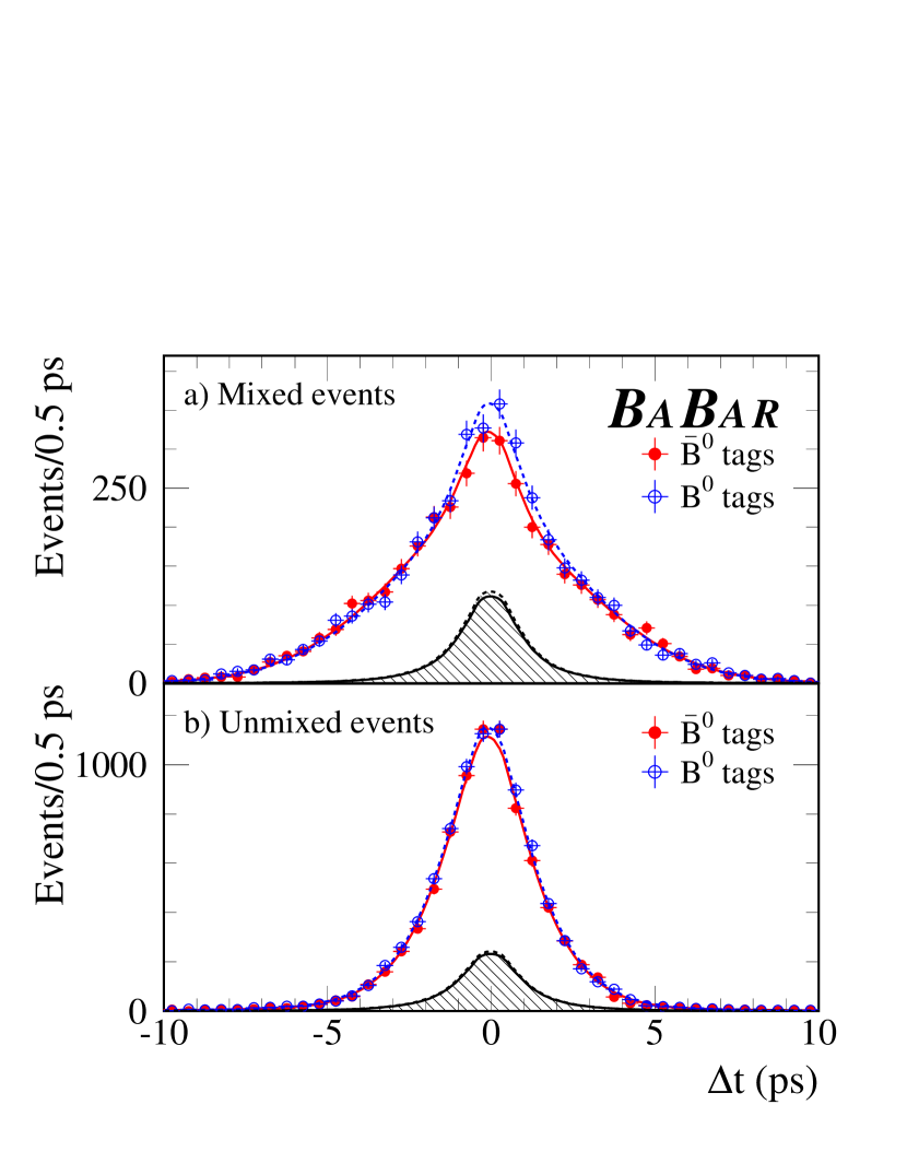
Figure 2: The $\Delta t$ distributions for (a) mixed and (b) unmixed $B_{\rm flav}$ events with a $B^{0}$ tag or with a $\kern 1.79993pt\overline{\kern-1.79993ptB}{}^{0}$ tag in the signal region, $m_{\rm ES}>5.27$ ${\mathrm{\,Ge\kern-1.00006ptV\!/}c^{2}}$. The solid (dashed) curves represent the fit projection in $\Delta t$ based on the individual signal and background probabilities and the event-by-event $\Delta t$ uncertainty for $\kern 1.79993pt\overline{\kern-1.79993ptB}{}^{0}$ ($B^{0}$) tags. The shaded area shows the background contribution to the distributions.

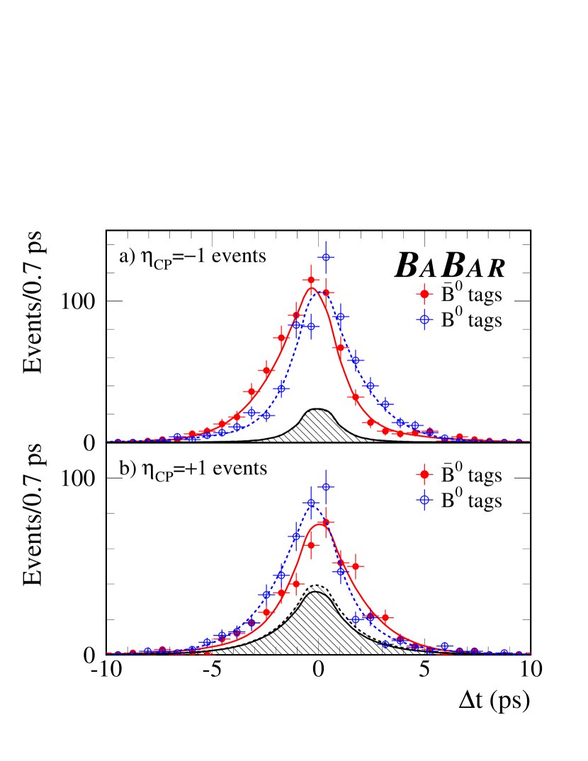
Figure 3: The $\Delta t$ distributions for (a) $B_{{C\!P}K^{0}_{\scriptscriptstyle S}}$ and (b) $B_{{C\!P}K^{0}_{\scriptscriptstyle L}}$ events with a $B^{0}$ tag or with a $\kern 1.79993pt\overline{\kern-1.79993ptB}{}^{0}$ tag in the signal region, $m_{\rm ES}>5.27$ ${\mathrm{\,Ge\kern-1.00006ptV\!/}c^{2}}$ for $B_{{C\!P}K^{0}_{\scriptscriptstyle S}}$ candidates and $|\Delta E|<10$ $\mathrm{\,Me\kern-1.00006ptV}$ for $B_{{C\!P}K^{0}_{\scriptscriptstyle L}}$ events. The solid (dashed) curves represent the fit projection in $\Delta t$ based on the individual signal and background probabilities and the event-by-event $\Delta t$ uncertainty for $\kern 1.79993pt\overline{\kern-1.79993ptB}{}^{0}$ ($B^{0}$) tags. The shaded area shows the background contribution to the distributions.

IX Cross-checks and validation studies

We use data and Monte Carlo samples to perform validation studies of the analysis technique. The Monte Carlo tests include studies with parameterized fast Monte Carlo as well as full GEANT4-simulated samples. Checks with data are performed with control samples, where no $\Delta\Gamma$ and $C\!P$-, $T$-, and $C\!PT$-violating effects are expected. Other checks are made by analyzing the actual data sample, but using alternative tagging, vertexing, and fitting configurations.

IX.1 Monte Carlo Simulation Studies

A test of the fitting procedure is performed with parameterized Monte Carlo simulations consisting of 300 experiments generated with a sample size and composition corresponding to that of the data. The mistag probabilities and $\Delta t$ distributions are generated according to the model used in the likelihood function. The physics parameters are generated according to the values found in the data . The nominal fit is then performed on each of these experiments. Each experiment uses the set of $m_{\rm ES}$ ($\Delta E$) and $\sigma_{\Delta t}$ values observed in the non-$K^{0}_{\scriptscriptstyle L}$ ($K^{0}_{\scriptscriptstyle L}$) sample. The r.m.s. spread of the residual distributions for all physics parameters (where the residual is defined as the difference between the fitted and generated values) is found to be consistent, within 10%, with the mean (Gaussian) statistical errors reported by the fits. Moreover, it has been verified using these experiments that the asymmetric 68% and 90% confidence-level intervals obtained from the fits provide the correct statistical coverage.

In all cases, the mean values of the residual distributions are consistent with no measurement bias. A systematic error due to the limited precision of this study is assigned to each physics parameter. The statistical errors on all the physics parameters (Table 11) and the calculated correlation coefficients among them (Tables 12 and 13), extracted from the fit are consistent with the range of values obtained from these experiments. We find that 24% of the fits result in a value of the log-likelihood that is greater (better) than that found in data.

In addition, samples of signal and background Monte Carlo events generated with a full detector simulation are used to validate the measurement. The largest samples are generated with $\Delta\Gamma/\Gamma$, $|q/p|-1$, and ${\mathsf{z}}$ all equal to zero, but additional samples are also produced with relatively large values of these parameters. Other values (including those measured in the data) are generated with reweighting techniques. The signal Monte Carlo events are split into samples whose size and proportions of $B_{\rm flav}$, $B_{{C\!P}K^{0}_{\scriptscriptstyle S}}$, and $B_{{C\!P}K^{0}_{\scriptscriptstyle L}}$  are similar to those of the actual data set. To check whether the selection criteria or the analysis and fitting procedures introduce any bias in the measurements, the fit (to signal alone) is then carried out on these experiments, allowing for $C\!PT$ violation. The small combinatorial background in these signal samples is suppressed by restricting the fit to the events in the signal region. Fits to a sample without background, using the true $\Delta t$ distribution and true tagging information, are also performed. The means of the residual distributions from all these experiments for all the physics parameters are consistent with zero, confirming that there is no measurement bias. The r.m.s. spreads are consistent with the average reported errors. A systematic error is assigned to each physics parameter corresponding to the limited Monte Carlo statistics for this test.

The effect of backgrounds is evaluated by adding an appropriate fraction of background events to the signal Monte Carlo sample and performing the fit. The $B_{C\!P}$ background samples are obtained either from simulated $B\rightarrow{J\mskip-3.0mu/\mskip-2.0mu\psi\mskip 2.0mu}X$ events or $\Delta E$ sidebands in data, while the $B_{\rm flav}$ backgrounds are obtained from generic $B\kern 1.79993pt\overline{\kern-1.79993ptB}{}$ Monte Carlo. We find no evidence for bias in any of the physics parameters.

IX.2 Cross-checks with Data

We fit subsamples defined by tagging category or data taking period. Fits using only the $B^{0}\rightarrow D^{(*)-}X^{+}$ or $B^{0}\rightarrow{J\mskip-3.0mu/\mskip-2.0mu\psi\mskip 2.0mu}K^{*0}(K^{+}\pi^{-})$ channels for $B_{\rm flav}$, and only $B_{{C\!P}K^{0}_{\scriptscriptstyle S}}$ or only $B_{{C\!P}K^{0}_{\scriptscriptstyle L}}$ for $B_{C\!P}$ are also performed. We find no statistically significant differences in the results for the different subsets. We also vary the maximum allowed values of $|\Delta t|$ between 5 and 30${\rm\,ps}$, and of $\sigma_{\Delta t}$ between 0.6 and 2.2${\rm\,ps}$. Again, we do not find statistically significant changes in the physics parameters.

In order to verify that the results are stable under variation of the vertex algorithm used in the measurement of $\Delta t$, we use alternative (less powerful) methods, described in Sec. VIII.C.5 in Ref. ref:babar-stwob-prd . To reduce statistical fluctuations due to different events being selected, the comparison between the alternative and nominal methods is performed using only the events accepted by both methods. Observed variations are small compared with the systematic error assigned to the resolution function (see Sec. X).

The stability of the results under variation of the tagging algorithm is studied by repeating the fit using the tagging algorithm described in Sec. IV in Ref. ref:babar-stwob-prd . The algorithm used in that analysis has an effective tagging efficiency $Q=\sum_{\alpha}\tau^{\alpha}\left(1-2w^{\alpha}\right)^{2}$ about 7% lower than the one used here. The variations observed in the physics parameters are consistent with the statistical differences.

The average $B^{0}$ lifetime is fixed in the nominal fit to the PDG value ref:pdg2002 . This value is obtained by averaging measurements based on flavor-eigenstate samples and by assuming negligible effects from $\Delta\Gamma/\Gamma$, $|q/p|$, and ${\mathsf{z}}$. Measurements that do not use tagged events are largely insensitive to $|q/p|$ and ${\mathsf{z}}$, but would be affected, at second order, by a non-zero value of $\Delta\Gamma/\Gamma$, as discussed in Sec. II. Therefore we do not expect sizeable effects from the fixed average $B^{0}$ lifetime. However, to check the consistency of the result, the fit is repeated with the average lifetime left free. The resulting $\tau_{B}$ is about one standard deviation below the nominal value assumed in our analysis, taking into account the statistical error from the fit and the present $\tau_{B}$ uncertainty. As described in Sec. X.3, a systematic error is assigned using the variation of each physics parameter when the fit is repeated with $\tau_{B}$ fixed to the value obtained when it is floated, which corresponds to a change of about twice the present PDG error ($\pm 0.032$${\rm\,ps}$).

Similarly, fits with $r_{C\!P}$ free have been performed. The resulting $r_{C\!P}$ value is consistent with unity (the fixed nominal value) within one standard deviation (statistical only). As described in Sec. X.3, systematic errors due to fixing $r_{C\!P}$ at unity are set by changing $r_{C\!P}$ by twice the statistical uncertainty determined by leaving it free in the fit ($\pm 10\%$). The resulting variation in each parameter is taken as the systematic error.

The robustness of the fit is also tested by modifying the nominal PDF normalization, as described by Eq. (37), so that the analysis is insensitive to the relative number of $B^{0}$ and $\kern 1.79993pt\overline{\kern-1.79993ptB}{}^{0}$ tagged events. As a consequence, the statistical error on $|q/p|$ is dramatically increased, since the sensitivity to this parameter comes largely from the differences in time-integrated $B^{0}$ and $\kern 1.79993pt\overline{\kern-1.79993ptB}{}^{0}$ rates. In addition, the fit is also performed assuming an independent set of resolution function parameters for each tagging category. In all cases the results are consistent with the nominal fit results. Finally, the tagging efficiencies $\tau^{\alpha}$ are alternatively determined for each sample ($B_{\rm flav}$, $B_{{C\!P}K^{0}_{\scriptscriptstyle S}}$ and $B_{{C\!P}K^{0}_{\scriptscriptstyle L}}$) separately, rather than using a common estimate from the $B_{\rm flav}$ sample, as in the nominal fit. The changes in the values of the physics parameters are negligible.

Control samples in data from $B^{+}$ decays (treated in a way analogous to that described in Sec. IV) are also used to validate the analysis technique, since in these samples we expect zero values for $\Delta\Gamma/\Gamma$, $|q/p|-1$ and ${\mathsf{z}}$. For the $B_{\rm flav}$ sample we use the $B^{+}\rightarrow\kern 1.99997pt\overline{\kern-1.99997ptD}{}^{0}\pi^{+},\kern 1.99997pt\overline{\kern-1.99997ptD}{}^{*0}\pi^{+}$ decay channels, and for the $B_{C\!P}$ sample the decays of charged-$B$ mesons to charmonium plus a charged $K$ or $K^{*}$ (see Table 6). The check is performed by fixing $\Delta m=0$ and $|q/p|=1$ in the $B_{\rm flav}$ sample, and assuming maximal mixing ($\Delta m=0.489$ ps^-1 ref:pdg2002 ) in the $B_{C\!P}$ sample, and fitting for $\mathop{\rm Im}\lambda_{C\!P}/|\lambda_{C\!P}|$, $\mathop{\rm{sgn}}(\mathop{\rm Re}\lambda_{C\!P})\Delta\Gamma/\Gamma$, $\left(\mathop{\rm Re}\lambda_{C\!P}/|\lambda_{C\!P}|\right)\mathop{\rm Re}{\mathsf{z}}$ and $\mathop{\rm Im}{\mathsf{z}}$. No statistically significant deviations from zero are observed.

X Systematic uncertainties

We estimate systematic uncertainties with studies performed on both data and Monte Carlo simulation samples. A summary of the sources of non-negligible uncertainties is shown in Table 14. In the following, the individual contributions are referenced by the lettered lines in the Table.

Table 14: Summary of systematic uncertainties on the measurements of $\mathop{\rm{sgn}}(\mathop{\rm Re}\lambda_{C\!P})\Delta\Gamma/\Gamma$, $|q/p|$, $\left(\mathop{\rm Re}\lambda_{C\!P}/|\lambda_{C\!P}|\right)\mathop{\rm Re}{\mathsf{z}}$, and $\mathop{\rm Im}{\mathsf{z}}$.

Systematics source	$\mathop{\rm{sgn}}(\mathop{\rm Re}\lambda_{C\!P})\Delta\Gamma/\Gamma$	$|q/p|$	$\left(\mathop{\rm Re}\lambda_{C\!P}/|\lambda_{C\!P}|\right)\mathop{\rm Re}{\mathsf{z}}$	$\mathop{\rm Im}{\mathsf{z}}$
Likelihood fit procedure
(a) Parameterized MC test	$\phantom{<}0.003$	$\phantom{<}0.001$	$\phantom{<}0.003$	$\phantom{<}0.003$
(b) GEANT4-simulation test	$\phantom{<}0.005$	$\phantom{<}0.007$	$\phantom{<}0.004$	$\phantom{<}0.016$
$\Delta t$ resolution function
(c) Resolution function parameterization	$\phantom{<}0.007$	$\phantom{<}0.001$	$\phantom{<}0.008$	$\phantom{<}0.003$
(d) $z$ scale and boost	$\phantom{<}0.003$	$\phantom{<}0.001$	$\phantom{<}0.002$	$<0.001$
(e) Beam spot	$\phantom{<}0.008$	$\phantom{<}0.002$	$\phantom{<}0.001$	$\phantom{<}0.011$
(f) SVT alignment	$\phantom{<}0.006$	$\phantom{<}0.001$	$\phantom{<}0.001$	$\phantom{<}0.011$
(g) Outliers	$\phantom{<}0.002$	$<0.001$	$<0.001$	$<0.001$
Signal properties
(h) Average $B^{0}$ lifetime	$\phantom{<}0.004$	$\phantom{<}0.001$	$\phantom{<}0.004$	$<0.001$
(i) Direct $C\!P$ violation	$\phantom{<}0.002$	$\phantom{<}0.004$	$\phantom{<}0.001$	$\phantom{<}0.003$
(j) $\rm DCS$ decays	$\phantom{<}0.008$	$\phantom{<}0.004$	$\phantom{<}0.032$	$\phantom{<}0.006$
(k) Residual charge asymmetries	$\phantom{<}0.005$	$\phantom{<}0.006$	$\phantom{<}0.004$	$\phantom{<}0.006$
Background properties
(l) Signal probability	$\phantom{<}0.002$	$\phantom{<}0.001$	$\phantom{<}0.002$	$\phantom{<}0.001$
(m) Fraction of peaking background	$<0.001$	$<0.001$	$\phantom{<}0.004$	$<0.001$
(n) $\Delta t$ structure	$\phantom{<}0.002$	$\phantom{<}0.001$	$\phantom{<}0.001$	$\phantom{<}0.001$
(o) $\Delta\Gamma$/$C\!P$/$T$/$C\!PT$/Mixing/$\rm DCS$ content	$\phantom{<}0.001$	$\phantom{<}0.002$	$\phantom{<}0.002$	$<0.001$
(p) Residual charge asymmetry	$<0.001$	$\phantom{<}0.001$	$<0.001$	$<0.001$
(q) $K^{0}_{\scriptscriptstyle L}$-specific systematic errors	$\phantom{<}0.004$	$<0.001$	$\phantom{<}0.004$	$\phantom{<}0.003$
Total systematic uncertainties	$\phantom{<}0.018$	$\phantom{<}0.011$	$\phantom{<}0.034$	$\phantom{<}0.025$

X.1 Likelihood Fit Procedure

Several sources of systematic uncertainties due to the likelihood fit procedure are considered. We include the results from the tests performed using the parameterized Monte Carlo sample (a) and the full GEANT4 signal Monte Carlo sample (b), as described in Sec. IX.1. No statistically significant bias (mean of the residual distributions) is observed. Thus, we assign a systematic error equal to the statistical uncertainty on the bias. No corrections are applied to the central values extracted from the fit to the data. Note that the GEANT4 contribution accounts for residual differences between the $B_{\rm flav}$, $B_{{C\!P}K^{0}_{\scriptscriptstyle S}}$, and $B_{{C\!P}K^{0}_{\scriptscriptstyle L}}$ samples in the mistag probability, resolution function, and $\nu$ and $\mu^{\alpha}$ parameters. It also includes residual differences in $\Delta t$ resolution for correct and wrong tags.

We also consider the impact on the measured physics parameters of normalizing the time-dependent PDFs to the full interval $-\infty<\Delta t<\infty$. The effect is evaluated by repeating the fit using a normalization in the range defined by the $\Delta t$ cut. Finally, the fixed tagging efficiencies are varied within their statistical uncertainties. The two contributions are negligible.

X.2 $\Delta t$ Resolution Function

The $\Delta t$ resolution model used in the analysis, consisting of the sum of three Gaussian distributions, is expected to be flexible enough to represent the experimental resolutions. To assign a systematic error for this assumption we use the alternative model described in Sec. VI, with a Gaussian distribution plus the same Gaussian convolved with one exponential function, for both signal and background. The results for all physics parameters obtained from the two resolution models are consistent and we assign the difference of central values as a systematic uncertainty (c).

In addition, a number of parameters that are inherent to the determination of $\Delta t$ are varied according to known uncertainties. The PEP-II boost, estimated from the beam energies, has an uncertainty of 0.1% ref:babar-nim . The absolute $z$-scale uncertainty is evaluated to be less than 0.4%. This estimate is obtained by measuring the beam pipe dimensions with scattered protons and comparing to optical survey data. Therefore, the boost and $z$-scale systematic uncertainties are evaluated conservatively by varying by $\pm 0.6\%$ the reconstructed $\Delta t$ and $\sigma_{\Delta t}$ (d). As the beam spot is much smaller in the vertical than in the horizontal dimension, its vertical position and size is more relevant in the vertex fits. Hence the uncertainty on the position and size of the beam spot used in the vertex fits is taken into account by changing the vertical position by up to 40$\,\mu\rm m$ and increasing the vertical size from 10$\,\mu\rm m$ to 60$\,\mu\rm m$ (e). Finally, the systematic uncertainty due to possible SVT internal misalignment is evaluated by applying a number of possible misalignment scenarios to a sample of simulated events and comparing the values of the fitted physics parameters from these samples to the case of perfect alignment (f).

Fixing the width and bias of the outlier Gaussian distribution in the resolution function to 8${\rm\,ps}$ and 0${\rm\,ps}$, respectively, is a potential source of bias. To estimate the corresponding systematic uncertainty we add in quadrature the variation observed in the physics parameters when the bias changes by $\pm$5${\rm\,ps}$, the width varies between 6${\rm\,ps}$ and 12${\rm\,ps}$, and the outlier distribution is assumed to be flat (g).

X.3 Signal Properties

As described in Sec. IX.2, the uncertainty from fixing the average $B^{0}$ lifetime is evaluated by changing its central value by $(\pm 0.032{\rm\,ps})^{-1}$ (h), twice the PDG error ref:pdg2002 . Possible direct $C\!P$ violation in the $B_{C\!P}$ sample is taken into account by varying $r_{C\!P}$ by $\pm 10\%$ (i).

Systematic uncertainties related to $\rm DCS$ decays arise because we fix the real parts of $\lambda_{Bt}$, $\overline{\lambda}_{{\kern 1.25995pt\overline{\kern-1.25995ptB}{}t}}$, $\lambda_{{Bf}}$, and $\overline{\lambda}_{{\kern 1.25995pt\overline{\kern-1.25995ptB}{}f}}$ to zero. In order to evaluate this contribution, we generate samples of parameterized Monte Carlo samples tuned to the data sample, scanning the $\rm DCS$-decay phases over their full allowed range (0-2$\pi$) and assuming a single hadronic decay channel contributing to the $B_{\rm tag}$ and to the $B_{\rm flav}$. Samples are generated with values of $|\overline{A}_{Bt}/A_{Bt}|$ and $|\overline{A}_{{Bf}}/A_{{Bf}}|$ equal to 0 and 0.04, corresponding to 100% variation of the value 0.02 used in the nominal fit. For the Lepton tagging category, dominated by semileptonic $B$ decays, we assume $\lambda_{Bt}$ to be zero. While the ratio of CKM matrix elements leads to the nominal value $|\overline{A}_{Bt}/A_{Bt}|=|\overline{A}_{{Bf}}/A_{{Bf}}|=0.02$, this is not a reliable estimate for any single decay mode. Examination of the $\rm DCS$ charmed-meson decay $D^{0}\rightarrow K^{+}\pi^{-}$ shows good agreement with expectations from CKM matrix elements, albeit with large uncertainties, but the singly-$\rm CKM$-suppressed decays $D^{0}\rightarrow\pi^{+}\pi^{-}$ and $D^{0}\rightarrow K^{+}K^{-}$ show deviations as large as a factor of two. However, when we sum over many channels, as we do here both for tagging states and for flavor eigenstates, quark-level predictions are much more reliable than they are for a single channel. Allowing for 100% variation from the nominal value of 0.02 is thus conservative.

Using the fit results from all these samples, we determine the offsets with respect to the generated value and its statistical uncertainty, for a complete sampling of $\rm DCS$-decay phases. The systematic error assigned is the largest value among all configurations (j). This is the dominant source of systematic uncertainty for the measurement of $\left(\mathop{\rm Re}\lambda_{C\!P}/|\lambda_{C\!P}|\right)\mathop{\rm Re}{\mathsf{z}}$ and is due primarily to the influence of $\rm DCS$ decays in the tagging-$B$ meson. The effect of using a single effective channel for the flavor and all tagging category states has been estimated by splitting the $B_{\rm flav}$ and $B_{\rm tag}$ samples generated with the parameterized Monte Carlo into equally sized subsamples. For the different combinations of $\rm DCS$-decay phases, the observed offset is about the average of the biases obtained using the single effective channel. Therefore, the largest offset among all configurations is smaller than that observed for a single channel. This shows that our prescription to describe the effects from $\rm DCS$ decays and to assign the systematic uncertainties assuming a single effective channel is conservative.

Charge asymmetries induced by a difference in the detector response for positive and negative tracks are included in the PDF and extracted together with the other parameters from the time-dependent analysis. Thus, they do not contribute to the systematic error, but rather are incorporated into the statistical error at a level determined by the size of the $B_{\rm flav}$ data sample. Nevertheless, in order to account for any possible residual effect, we assign a systematic uncertainty as follows. We rerun the $B$ reconstruction, vertex-finding, and tagging algorithms after removing randomly and uniformly (no momentum or angular dependence) 5% of positive and, separately, negative tracks in the full Monte Carlo sample. This value of 5% is on average more than a factor of three larger than the precision with which the parameters $\nu^{\rm sig}$ and $\mu^{\alpha,\rm sig}$ have been measured in the data. Half the difference between the results obtained for positive and negative tracks is assigned as a systematic error (k).

X.4 Background Properties

The event-by-event signal probability $p^{\alpha}_{{\rm rec}}(m_{\rm ES})$ for $B_{\rm flav}$ and $B_{{C\!P}K^{0}_{\scriptscriptstyle S}}$ samples is fixed to the values obtained from the $m_{\rm ES}$ fits. We compare the results from the nominal fit to the values obtained by varying all the $m_{\rm ES}$ distribution parameters by $\pm 1\sigma$, taking into account their correlations. This is performed simultaneously for all tagging categories, and independently for the $B_{\rm flav}$ and $B_{{C\!P}K^{0}_{\scriptscriptstyle S}}$ samples. As an alternative, we also use a flat signal probability distribution: events belonging to the sideband region ($m_{\rm ES}$$<$5.27 ${\mathrm{\,Ge\kern-1.00006ptV\!/}c^{2}}$) are assigned a signal probability of zero, while we give a signal probability equal to the purity of the corresponding sample to signal region events ($m_{\rm ES}$$>$5.27 ${\mathrm{\,Ge\kern-1.00006ptV\!/}c^{2}}$). The differences among fitted physical parameters with respect to the default method are found to be consistent. We determine the systematic error due to this parameterization by varying the signal probability by its statistical error. The final systematic error is taken to be the larger of the one-sigma variations found for the two methods (l). The uncertainty on the fraction of peaking background is estimated by varying the fractions according to their uncertainties separately for the $B_{\rm flav}$ sample and each $B_{{C\!P}K^{0}_{\scriptscriptstyle S}}$ decay mode (m). The effective $\eta_{C\!P}$ of the $B_{{C\!P}K^{0}_{\scriptscriptstyle S}}$ peaking background, assumed to be zero in the nominal fit, is also varied between $+1$ and $-1$ and the variations induced are negligible.

Another source of systematic uncertainty is the assumption that the $\Delta t$ behavior of the combinatorial background in the $m_{\rm ES}$ sideband region is the same as it is in the signal region. However, the background composition changes gradually as a function of $m_{\rm ES}$, since the fraction due to continuum production slowly decreases as $m_{\rm ES}$ increases. To study the impact of variable $\Delta t$ behavior over the $m_{\rm ES}$ range, we vary the lower edge of the $m_{\rm ES}$ distributions from 5.20${\mathrm{\,Ge\kern-1.00006ptV\!/}c^{2}}$ to 5.27${\mathrm{\,Ge\kern-1.00006ptV\!/}c^{2}}$, simultaneously for the $B_{\rm flav}$ and $B_{{C\!P}K^{0}_{\scriptscriptstyle S}}$ samples, observing good stability in the results. We also split the sideband region in seven equal slices each 10 ${\mathrm{\,Me\kern-1.00006ptV\!/}c^{2}}$ wide and repeat the fit in each of these slices. The results obtained for all physics parameters and $m_{\rm ES}$ slices are then linearly extrapolated to the $B$-mass signal region. The quadratic sum of the extrapolation and the error on it is assigned as a systematic uncertainty (n).

As described in Sec. VII, the likelihood fit assumes that there are no effects of $\Delta\Gamma$, $C\!P$, $T$ or $C\!PT$ violation, mixing, and $\rm DCS$ decays in the combinatorial background components ($B_{\rm flav}$ and $B_{{C\!P}K^{0}_{\scriptscriptstyle S}}$ samples) and in the non-${J\mskip-3.0mu/\mskip-2.0mu\psi\mskip 2.0mu}$  background ($B_{{C\!P}K^{0}_{\scriptscriptstyle L}}$ sample). To evaluate the effect of this assumption, we repeat the fit assuming for the background non-zero values of $\Delta\Gamma$, $|q/p|-1$, ${\mathsf{z}}$, $\mathop{\rm Im}\lambda_{C\!P}/|\lambda_{C\!P}|$, and $\Delta m$, and varying $\eta_{C\!P}$ of the background by $\pm 1$. The check is performed by introducing an independent set of physics parameters in the PDF and assuming maximal mixing and $C\!P$ violation ($\Delta m$ and $\mathop{\rm Im}\lambda_{C\!P}/|\lambda_{C\!P}|$ fixed to $0.489{\rm\,ps}^{-1}$ ref:pdg2002 and 0.75 ref:sin2b-babar , respectively). $\rm DCS$-decay effects are included by assuming the maximal values (0.04) of $|\overline{A}_{Bt}/A_{Bt}|$ and $|\overline{A}_{{Bf}}/A_{{Bf}}|$, and scanning all the possible values of the $B^{0}$ and $\kern 1.79993pt\overline{\kern-1.79993ptB}{}^{0}$ phases for $B_{\rm flav}$ and $B_{\rm tag}$. The systematic uncertainty is evaluated simultaneously for all these sources (o).

The systematic errors due to the $B^{+}$ decay rate are evaluated by varying its value by the PDG uncertainty ref:pdg2002 . The effect is negligible. The $B^{+}$ mistags and the differences in the fraction of $B^{+}$ and $B^{-}$ mesons that are tagged and reconstructed are varied according to their statistical errors as obtained from the fit to the $B^{+}$ data. These errors are found to be negligible.

Uncertainties from charge asymmetries in combinatorial background components (neglected in the nominal fit) are evaluated by repeating the fit with a new set of $\nu$ and $\mu^{\alpha}$ parameters. The measured values of $\nu$ and $\mu^{\alpha}$ are found to be compatible with zero and the variation of the physical parameters with respect to the nominal fit is assigned as a systematic error (p).

For the $B_{{C\!P}K^{0}_{\scriptscriptstyle L}}$ channel, the signal and non-${J\mskip-3.0mu/\mskip-2.0mu\psi\mskip 2.0mu}$ background fractions are varied according to their statistical uncertainties, obtained from the fit to the $\Delta E$ distribution. We also vary background parameters, including the ${J\mskip-3.0mu/\mskip-2.0mu\psi\mskip 2.0mu}X$ branching fractions, the assumed $\eta_{C\!P}$, the $\Delta E$ shape, and the fraction and effective lifetime of the prompt and non-prompt non-${J\mskip-3.0mu/\mskip-2.0mu\psi\mskip 2.0mu}$ components. The differences observed between data and Monte Carlo simulation for the $K^{0}_{\scriptscriptstyle L}$ angular resolution and for the fractions of $B^{0}\rightarrow{J\mskip-3.0mu/\mskip-2.0mu\psi\mskip 2.0mu}K^{0}_{\scriptscriptstyle L}$ events reconstructed in the EMC and IFR are used to evaluate a systematic uncertainty due to the simulation of the $K^{0}_{\scriptscriptstyle L}$  reconstruction. Finally, an additional contribution is assigned to the correction applied to Lepton events due to the observed differences in flavor tagging efficiencies in the ${J\mskip-3.0mu/\mskip-2.0mu\psi\mskip 2.0mu}$ sideband relative to $B_{\rm flav}$ and inclusive ${J\mskip-3.0mu/\mskip-2.0mu\psi\mskip 2.0mu}$ Monte Carlo samples. Conservatively, this error is evaluated by comparing the fit results with and without the correction. The total $B_{{C\!P}K^{0}_{\scriptscriptstyle L}}$-specific systematic error is evaluated by taking the quadratic sum of the individual contributions (q).

X.5 Summary of Systematic Uncertainties

All individual systematic contributions described above and summarized in Table 14 are added in quadrature. The dominant source of systematic error in the measurement of $\left(\mathop{\rm Re}\lambda_{C\!P}/|\lambda_{C\!P}|\right)\mathop{\rm Re}{\mathsf{z}}$ is due to our limited knowledge of the $\rm DCS$ decays, which also contributes significantly to the uncertainties on the other measurements. The limited Monte Carlo sample size is a dominant source of systematic error for $|q/p|$, $\mathop{\rm Im}{\mathsf{z}}$, and to a lesser extent for $\mathop{\rm{sgn}}(\mathop{\rm Re}\lambda_{C\!P})\Delta\Gamma/\Gamma$. Residual charge asymmetries, mainly due to limited simulation statistics, dominate the systematic error on $|q/p|$. Our limited knowledge of the beam spot and SVT alignment reflects significantly on $\mathop{\rm Im}{\mathsf{z}}$ and $\mathop{\rm{sgn}}(\mathop{\rm Re}\lambda_{C\!P})\Delta\Gamma/\Gamma$. The systematic error on $\mathop{\rm{sgn}}(\mathop{\rm Re}\lambda_{C\!P})\Delta\Gamma/\Gamma$  receives a non-negligible contribution from our incomplete understanding of the resolution function.

The systematic uncertainties on $\mathop{\rm{sgn}}(\mathop{\rm Re}\lambda_{C\!P})\Delta\Gamma/\Gamma$ and $|q/p|$ when $C\!PT$ invariance is assumed are evaluated similarly, and found to be consistent, within the statistical fluctuations of the Monte Carlo simulation, with those found for the analysis when $C\!PT$ violation is allowed.

XI Summary and discussion of results

The conventional analyses of mixing and $C\!P$ violation in the neutral-$B$-meson system neglect possible contributions from several sources that are expected to be small. These include the difference of the decay rates of the two neutral-$B$-meson mass eigenstates, the $C\!P$- and $T$-violating quantity $|q/p|-1$, and potential $C\!PT$ violation. To measure or extract limits on these quantities requires the full expressions for time dependence in mixing and $C\!P$ violation and consideration of systematic effects that might mimic the fundamental asymmetries we seek to measure. Such systematic effects could be induced by detector charge asymmetries, different resolution functions for positive and negative $\Delta t$, and $\rm DCS$ decays for both fully reconstructed final flavor states and nonleptonic tagging states.

A limit on the decay-rate difference of $|\Delta\Gamma/\Gamma|<80\%$ at 95% confidence-level was obtained by CLEO ref:cleochid using the time-integrated mixing parameter $\chi_{d}$ and the mass difference $\Delta m$ extracted under the assumption $\Delta\Gamma=0$. Using $Z^{0}$ decays, DELPHI ref:delphi has recently performed a time-dependent study of semileptonic $B$ decays inclusively reconstructed. Assuming no $C\!P$, $T$, or $C\!PT$ violation in mixing, they quote the limit $|\Delta\Gamma/\Gamma|<18\%$ at 95% confidence-level.

Both $|q/p|$ and $\mathop{\rm Im}{\mathsf{z}}$ were measured by OPAL ref:otherCPTBtests , using $Z^{0}$ decays to $b{\overline{b}}$ pairs and assuming $\Delta\Gamma=0$. Neutral-$B$-meson oscillations were studied by observing a single lepton indicative of a $B$ decay and the jet-charge associated with both the jet containing the lepton and the other jet. Because the multiparticle final states provide essentially uncorrelated $B$ mesons, the issue of $\rm DCS$ decays is obviated. The results were $\mathop{\rm Re}\,\epsilon_{B}=0.006\pm 0.010\pm 0.006$, equivalent to $|q/p|=0.988\pm 0.020\pm 0.012$, and $\mathop{\rm Im}\epsilon_{B}=-0.020\pm 0.016\pm 0.006$, equivalent to $\mathop{\rm Im}{\mathsf{z}}=0.040\pm 0.032\pm 0.012$. Combining the earlier $|q/p|$ measurements, all obtained assuming $\Delta\Gamma=0$, gives $|q/p|=0.9993\pm 0.0064$ ref:pdg2003 . Belle has used dilepton events to obtain limits on $C\!PT$ violation ref:belle_dilepton . Assuming that $\Delta\Gamma=0$ and that $C\!P$ violation in mixing can be ignored, they find $\mathop{\rm Re}\cos\theta=-\mathop{\rm Re}{\mathsf{z}}=0.00\pm 0.12\pm 0.02$ and $\mathop{\rm Im}\cos\theta=-\mathop{\rm Im}{\mathsf{z}}=0.03\pm 0.01\pm 0.03$.

Our analysis of approximately 31,000 fully reconstructed flavor eigenstates and 2,600 $C\!P$ eigenstates sets new limits on the difference of decay rates of $B^{0}$ mesons, and on the $C\!P$, $T$, and $C\!PT$ violation intrinsic to $B^{0}{\kern-1.60004pt\kern 1.79993pt\overline{\kern-1.79993ptB}{}^{0}}$ mixing. The six independent parameters governing oscillations ($\Delta m$, $\Delta\Gamma/\Gamma$), $C\!PT$ and $C\!P$ violation ($\mathop{\rm Re}{\mathsf{z}}$, $\mathop{\rm Im}{\mathsf{z}}$), and $C\!P$ and $T$ violation ($\mathop{\rm Im}\lambda_{C\!P}$, $|q/p|$) are extracted from a single fit of both fully reconstructed $C\!P$ and flavor events, tagged and untagged. This provides the sensitivity required to separate all effects we seek from asymmetries in detector response and from potentially obscuring correlations in the decays of the two $B$ mesons. The results are

$$\begin{array}[]{l}\mathop{\rm{sgn}}(\mathop{\rm Re}\lambda_{C\!P})\Delta\Gamma/\Gamma=\\ \quad-0.008\pm 0.037\mathrm{(stat.)}\pm 0.018\mathrm{(syst.)}[-0.084,0.068]~{},\\ |q/p|=\\ \quad\phantom{+}1.029\pm 0.013\mathrm{(stat.)}\pm 0.011\mathrm{(syst.)}[\phantom{+}1.001,1.057]~{},\\ \left(\mathop{\rm Re}\lambda_{C\!P}/|\lambda_{C\!P}|\right)\mathop{\rm Re}{\mathsf{z}}=\\ \quad\phantom{+}0.014\pm 0.035\mathrm{(stat.)}\pm 0.034\mathrm{(syst.)}[-0.072,0.101]~{},\\ \mathop{\rm Im}{\mathsf{z}}=\\ \quad\phantom{+}0.038\pm 0.029\mathrm{(stat.)}\pm 0.025\mathrm{(syst.)}[-0.028,0.104]~{}.\\ \end{array}$$

The values in square brackets indicate the 90% confidence-level intervals. When estimating the limits we also evaluate multiplicative contributions to the systematic error, adding them in quadrature with the additive systematic uncertainties. Fig. 4 shows the results in the $(\mbox{$|q/p|$-1},|{\mathsf{z}}|)$ plane, compared to the BABAR measurement of $|q/p|$ made with dilepton events, $|q/p|=0.998\pm 0.006\pm 0.007$ ref:babardileptonTviolation , and to the Standard Model expectations. The region shown for this analysis is obtained by simulating a large number of experiments using the measured covariance matrix for the parameters $\mathop{\rm Re}{\mathsf{z}}$, $\mathop{\rm Im}{\mathsf{z}}$, and $|q/p|$, and is constrained to lie within the physical region $|{\mathsf{z}}|\geq 0$. The three-dimensional distribution in $\mathop{\rm Re}{\mathsf{z}},\mathop{\rm Im}{\mathsf{z}}$, and $|q/p|$ is projected onto the two dimensions $|{\mathsf{z}}|^{2}$ and $|q/p|$. The boundary is then chosen to exclude the maximal region. For simplicity in the figure, we display $|{\mathsf{z}}|$ rather than $|{\mathsf{z}}|^{2}$. The dilepton measurement constrains $|q/p|$ without assumptions on the value of $|{\mathsf{z}}|$. The region in this case is obtained from the $\Delta\chi^{2}=1$ limits for this single variable.

Figure 4: Favored regions at 68% confidence level in the $(|q/p|-1,|{\mathsf{z}}|)$ plane determined by this analysis and by the BABAR measurement of the dilepton asymmetry ref:babardileptonTviolation . The axis labels reflect the requirements that both $C\!P$ and $T$ be violated if $|q/p|\neq 1$ and that both $C\!P$ and $C\!PT$ be violated if $|{\mathsf{z}}|\neq 0$. The Standard Model expectation for $|q/p|$ is obtained from Refs. ref:ciuchini ; ref:absqopSM ; ref:beneke .

Assuming $C\!PT$ invariance the results are

$$\begin{array}[]{l}\mathop{\rm{sgn}}(\mathop{\rm Re}\lambda_{C\!P})\Delta\Gamma/\Gamma=\\ \quad-0.009\pm 0.037\mathrm{(stat.)}\pm 0.018\mathrm{(syst.)}[-0.085,0.067]~{},\\ |q/p|=\\ \quad\phantom{+}1.029\pm 0.013\mathrm{(stat.)}\pm 0.011\mathrm{(syst.)}[\phantom{+}1.001,1.057]~{}.\end{array}$$

Figure 5: Constraints at 68% and 90% confidence level on the complex ratio $\Gamma_{12}/M_{12}$ of the effective Hamiltonian off-diagonal matrix elements governing neutral-$B$-meson oscillations as determined from the $\mathop{\rm{sgn}}(\mathop{\rm Re}\lambda_{C\!P})\Delta\Gamma/\Gamma$ and $|q/p|$ measurements of this analysis with ${\mathsf{z}}$ fixed to zero, compared to predictions of Standard Model calculations when other experimental inputs are used. The lower figure is an enlargement of the region around the origin. The bands in the lower figure are calculated using only the constraint obtained from the BABAR $\sin 2\beta$ measurement with $C\!P$ eigenstates like ${J\mskip-3.0mu/\mskip-2.0mu\psi\mskip 2.0mu}K^{0}_{\scriptscriptstyle S}$ ref:sin2b-babar . The fading out of the bands away from the origin indicates that these predictions are only valid for small $|\Gamma_{12}/M_{12}|$.

These results can be used to set constraints on the complex ratio $\Gamma_{12}/M_{12}$ when $C\!PT$ invariance is assumed, as shown in Fig. 5. Ellipses in the upper figure enclose the favored regions determined from the $\mathop{\rm{sgn}}(\mathop{\rm Re}\lambda_{C\!P})\Delta\Gamma/\Gamma$ and $|q/p|$ measurements of this analysis with ${\mathsf{z}}$ fixed to zero. Solid contours show the results assuming $\mathop{\rm Re}\lambda_{C\!P}>0$ (as expected in the Standard Model based on other experimental constraints), while dashed contours are for $\mathop{\rm Re}\lambda_{C\!P}<0$. Inner (outer) contours represent 68% (90%) confidence-level regions for two degrees of freedom. The lower figure is an enlargement of the region around the origin of the complex $\Gamma_{12}/M_{12}$ plane. The black region close to the origin of the complex plane in the upper and lower figures shows the predictions of Standard Model calculations when all available experimental inputs are used to constrain the ratio of CKM matrix elements $(V_{cb}V_{cd}^{*})/(V_{tb}V_{td}^{*})$. The bands in the lower figure are calculated using only the constraint $\sin 2\beta=0.741\pm 0.075$ obtained from the BABAR measurement with $C\!P$ eigenstates like ${J\mskip-3.0mu/\mskip-2.0mu\psi\mskip 2.0mu}K^{0}_{\scriptscriptstyle S}$ ref:sin2b-babar .

The decay-rate difference results can alternatively be expressed normalized to the mass difference $\Delta m$. Using the world-average value of $\Delta m$ ref:pdg2002 , the result allowing for $C\!PT$ violation (${\mathsf{z}}$ free) is

$$\begin{array}[]{l}\mathop{\rm{sgn}}(\mathop{\rm Re}\lambda_{C\!P})\Delta\Gamma/\Delta m=\\ \quad-0.011\pm 0.049\mathrm{(stat.)}\pm 0.024\mathrm{(syst.)}[-0.112,0.091]~{},\end{array}$$

and with $C\!PT$ invariance (${\mathsf{z}}=0$)

$$\begin{array}[]{l}\mathop{\rm{sgn}}(\mathop{\rm Re}\lambda_{C\!P})\Delta\Gamma/\Delta m=\\ \quad-0.012\pm 0.049\mathrm{(stat.)}\pm 0.024\mathrm{(syst.)}[-0.113,0.090]~{}.\end{array}$$

The parameters $\Delta m$ and $\mathop{\rm Im}\lambda_{C\!P}/|\lambda_{C\!P}|$ are free in the fit, so that recent $B$-factory $\Delta m$ results ref:dM-babar-had ; ref:dM-babar-dstlnu ; ref:dM-babar-dilep ; ref:dM-belle and our $\sin 2\beta$ analysis based on the same data sample ref:sin2b-babar provide a cross-check. The value of the $C\!P$- and $T$-violating parameter $\mathop{\rm Im}\lambda_{C\!P}/|\lambda_{C\!P}|$ increases by $+0.011$ when $C\!PT$ violation is allowed in the fit. This change is equal to 15% of the statistical uncertainty on $\mathop{\rm Im}\lambda_{C\!P}/|\lambda_{C\!P}|$ and is consistent with the correlations observed in the fit with $C\!PT$ violation.

The results are consistent with Standard Model expectations and with $C\!PT$ invariance. To date, these are the lowest limits on the difference of decay widths of $B^{0}$ mesons and the strongest test of $C\!PT$ invariance outside the neutral-kaon system ref:cptkaons . If we express the $C\!PT$ limits as ratios of the $C\!PT$-violating to the $C\!PT$-conserving terms we have

$$\frac{|\delta m|}{m}<1.0\times 10^{-14}~{},$$

$$-0.156<\frac{\delta\Gamma}{\Gamma}<0.042~{}$$

at the 90% confidence-level. The limit on $C\!P$ and $T$ violation in mixing is independent of and consistent with our previous measurement based on the analysis of inclusive dilepton events ref:babardileptonTviolation . All the other results are also consistent with previous analyses ref:dM-belle ; ref:cleochid ; ref:delphi ; ref:otherCPTBtests ; ref:pdg2002 ; ref:pdg2003 ; ref:belle_dilepton . All these measurements were obtained with more restrictive assumptions than those used here. While the Standard Model predictions for $\Delta\Gamma$ and $|q/p|$ are still well below our current limits and no $C\!PT$ violation is anticipated, higher precision measurements may still bring surprises.

XII Acknowledgments

We are grateful for the extraordinary contributions of our PEP-II colleagues in achieving the excellent luminosity and machine conditions that have made this work possible. The success of this project also relies critically on the expertise and dedication of the computing organizations that support BABAR. The collaborating institutions wish to thank SLAC for its support and the kind hospitality extended to them. This work is supported by the US Department of Energy and National Science Foundation, the Natural Sciences and Engineering Research Council (Canada), Institute of High Energy Physics (China), the Commissariat à l’Energie Atomique and Institut National de Physique Nucléaire et de Physique des Particules (France), the Bundesministerium für Bildung und Forschung and Deutsche Forschungsgemeinschaft (Germany), the Istituto Nazionale di Fisica Nucleare (Italy), the Foundation for Fundamental Research on Matter (The Netherlands), the Research Council of Norway, the Ministry of Science and Technology of the Russian Federation, and the Particle Physics and Astronomy Research Council (United Kingdom). Individuals have received support from the A. P. Sloan Foundation, the Research Corporation, and the Alexander von Humboldt Foundation.

Appendix A Efficiency asymmetries

The use of untagged data is essential for determining the asymmetries in the tagging and reconstruction efficiencies. To indicate how the various samples enter we provide a simple example using only time-integrated quantities. In practice we use a time-dependent analysis, which gives better precision because it uses more information.

Suppressing the indices for the tag category index $\alpha$ and the signal or background component $j$, and writing the reconstruction efficiencies as $\rho=\rho^{j}_{{Bf}},\,{\overline{\rho}}=\rho^{j}_{{\kern 1.25995pt\overline{\kern-1.25995ptB}{}f}}$ and the tagging efficiencies as $\tau=\tau^{\alpha,j}_{Bt},\,{\overline{\tau}}=\tau^{\alpha,j}_{{\kern 1.25995pt\overline{\kern-1.25995ptB}{}t}}$, Eq. (41) reads

$$\nu = \frac{\rho-{\overline{\rho}}}{\rho+{\overline{\rho}}}~{},$$

$$\mu = \frac{\tau-{\overline{\tau}}}{\tau+{\overline{\tau}}}~{}.$$ (42)

Using the numbers of signal events that are tagged and have a reconstructed $B^{0}$ ($X$), those tagged and having a $\kern 1.79993pt\overline{\kern-1.79993ptB}{}^{0}$ ($Y$), those untagged with a reconstructed $B^{0}$ ($Z$), and finally those untagged with a reconstructed $\kern 1.79993pt\overline{\kern-1.79993ptB}{}^{0}$ ($W$), we can determine the required asymmetries ref:babar-stwob-prd . To see this, note that if the total number of $B^{0}{\kern-1.60004pt\kern 1.79993pt\overline{\kern-1.79993ptB}{}^{0}}$ pairs is $N$, and neglecting $\Delta\Gamma$, $|q/p|-1$, and ${\mathsf{z}}$ corrections, there are

$$N_{u} = N(1+[1/(1+x^{2})])/2$$ (43)

unmixed events (i.e., $B^{0}{\kern-1.60004pt\kern 1.79993pt\overline{\kern-1.79993ptB}{}^{0}}$) and

$$N_{m} = N(1-[1/(1+x^{2})])/2$$ (44)

mixed events (i.e., $B^{0}B^{0}$ or $\kern 1.79993pt\overline{\kern-1.79993ptB}{}^{0}\kern 1.79993pt\overline{\kern-1.79993ptB}{}^{0}$), where $x=\Delta m/\Gamma$. Then we have

$$X = \rho\tau N_{m}/2+\rho{\overline{\tau}}N_{u}/2~{},$$

$$Y = {\overline{\rho}}\hskip 1.0pt{\overline{\tau}}N_{m}/2+{\overline{\rho}}\tau N_{u}/2~{},$$

$$Z = \rho(1-\tau)N_{m}/2+\rho(1-\overline{\tau})N_{u}/2~{},$$

$$W = {\overline{\rho}}(1-\overline{\tau})N_{m}/2+{\overline{\rho}}(1-\tau)N_{u}/2~{}.$$ (45)

Setting $U=X+Z$ and $V=Y+W$, we find

$$\nu=\frac{U-V}{U+V}~{}~{},~{}~{}~{}\mu=(1+x^{2})\frac{(Y/V)-(X/U)}{(Y/V)+(X/U)}~{}.$$ (46)

Corrections to these equations have to be applied due to non-zero values of $\Delta\Gamma$, $|q/p|-1$ and ${\mathsf{z}}$. The use of untagged events is therefore essential to the determination of $\nu$ and $\mu$.

References

(1)BABAR Collaboration, B. Aubert et al.,
Phys. Rev. Lett. 88, 221802 (2002).
(2)BABAR Collaboration, B. Aubert et al.,
Phys. Rev. D 67, 072002 (2003).
(3)BABAR Collaboration, B. Aubert et al.,
Phys. Rev. Lett. 88, 221803 (2002).
(4) Belle Collaboration, N.C. Hastings et al.,
Phys. Rev. D 67, 052004 (2003).
(5)BABAR Collaboration, B. Aubert et al., Phys. Rev. Lett. 89, 201802 (2002).
(6) Belle Collaboration, K. Abe et al., Phys. Rev. D 66, 071102(R) (2002).
(7) A.S. Dighe, T. Hurth, C.S. Kim, and T. Yoshikawa, Nucl. Phys. B 624, 377 (2002).
(8) M. Ciuchini, E. Franco, V. Lubicz, F. Mescia, and C. Tarantino, JHEP 0308, 031 (2003).
(9) CLEO Collaboration, B.H. Behrens et al., Phys. Lett. B 490, 36 (2000).
(10) DELPHI Collaboration, J. Abdallah et al., Eur. Phys. Jour. C 28, 155 (2003).
(11)BABAR Collaboration, B. Aubert et al., Phys. Rev. Lett. 88, 231801 (2002).
(12) S. Laplace, Z. Ligeti, Y. Nir, and G. Perez, Phys. Rev. D 65, 094040 (2002).
(13) M. Beneke, G. Buchalla, A. Lenz, and U. Nierste, Phys. Lett. B 576, 173 (2003).
(14) M. Kobayashi and A.I. Sanda, Phys. Rev. Lett. 69, 3139 (1992).
(15) D. Colladay and V.A. Kostelecký, Phys. Lett. B 344, 259 (1995);
V.A. Kostelecký and R. Van Kooten, Phys. Rev. D 54, 5585 (1996);
V.A. Kostelecký, Phys. Rev. D 64, 076001 (2001).
(16)M.C. Bañuls and J. Bernabéu,
Phys. Lett. B 464, 117 (1999); Nucl. Phys. B 590, 19 (2000).
(17) G. Lüders, Dansk. Math. Phys. Medd. 28, 5 (1954); Ann. Phys. 2, 1 (1957);
W. Pauli, Nuo. Cim. 6, 204 (1957);
R. Jost, Helv. Phys. Acta 30, 409 (1957);
F.J. Dyson, Phys. Rev. 110, 579 (1958);
R.F. Streater and A.S. Wightman, PCT, Spin and Statistics, and All That, Benjamin, New York, 1964.
(18) M.S. Berger and V.A. Kostelecký, Phys. Rev. D 65, 091701 (2002);
V.A. Kostelecký and R. Potting, Phys. Rev. D 51, 3923 (1995).
(19) KTeV Collaboration, A. Alavi-Harati et al., Phys. Rev. D 67, 012005 (2003);
CPLEAR Collaboration, A. Apostolakis et al., Phys. Lett. B 456, 297 (1999);
E773 Collaboration, B. Schwingenheuer et al., Phys. Rev. Lett. 74, 4376 (1995);
NA31 Collaboration, R. Carosi et al., Phys. Lett. B 237, 303 (1990).
(20) OPAL Collaboration, R. Ackerstaff et al., Z. Phys. C 76, 401 (1997).
(21)BABAR Collaboration, B. Aubert et al.,
arXiv:hep-ex/0311037, to appear in Phys. Rev. Lett.
(22) O. Long, M. Baak, R. Cahn, and D. Kirkby, Phys. Rev. D 68, 034010 (2003).
(23) Y. Grossman, A.L. Kagan, and Z. Ligeti, Phys. Lett. B 538, 327 (2002).
(24) CLEO Collaboration, G. Bonvicini et al., Phys. Rev. Lett. 84, 5940 (2000).
(25)BABAR Collaboration, B. Aubert et al.,
Phys. Rev. D 65, 091101 (2002).
(26) R. Fleischer and T. Mannel, Phys. Lett. B 506, 311 (2001).
(27)BABAR Collaboration, B. Aubert et al., Nucl. Instr. Meth. A 479, 1 (2002).
(28) S. Agostinelli et al., Nucl. Instr. Meth. A 506, 250 (2003).
(29)BABAR Collaboration, B. Aubert et al., Phys. Rev. D 66, 032003 (2002).
(30) ARGUS Collaboration, H. Albrecht et al., Z. Phys. C 48, 543 (1990).
(31) Particle Data Group, K. Hagiwara et al., Phys. Rev. D 66, 010001 (2002).
(32) 2003 partial update of Ref. ref:pdg2002 for edition 2004 (http://pdg.lbl.gov).
(33) Belle Collaboration, N.C. Hastings et al., Phys. Rev. D 67, 052004 (2003).