The CP-conserving triple-gauge-boson couplings, , , , , and are measured using hadronic and semi-leptonic W-pair events selected in 629 pb-1 of data collected at LEP with the L3 detector at centre-of-mass energies between and . The results are combined with previous L3 measurements based on data collected at lower centre-of-mass energies and with the results from single-W production and from events with a single-photon and missing energy. Imposing the constraints and , we obtain for the C and P conserving couplings the results:
Results from the analysis of fully leptonic W-pair decays are also given. All results are in agreement with the Standard Model expectations and confirm the existence of self-couplings among electroweak gauge bosons.
Submitted to Phys. Lett. B
1 Introduction
The non-Abelian structure of the electroweak theory [1] implies the existence of trilinear self couplings among gauge bosons. The vertices WW and ZWW are accessible at LEP through W-pair, single-W and single-photon production [2].
To lowest order, three Feynman diagrams contribute to W-pair production: the -channel and Z exchange and the -channel exchange. The -channel diagrams contain the WW and ZWW vertices. The WW vertex appears in one of the -channel Feynman diagrams contributing to single-W production, ; at LEP centre-of-mass energies, , the contribution from the similar diagram containing the ZWW vertex is negligible. The WW vertex also contributes to the process through photon production in W-boson fusion.
Assuming only Lorentz invariance, the most general form of the WW and ZWW vertices is parametrised in terms of seven complex triple-gauge-boson couplings (TGC’s) each [3]. Retaining only CP-conserving couplings and assuming electromagnetic gauge invariance, six real TGC’s remain, namely , , , , and . At tree level within the Standard Model, and . Except , these TGC’s also conserve C and P separately. The requirement of custodial symmetry leads to the relations and [4, 5], where is the weak mixing angle. When these constraints are applied, , and correspond to the operators in a linear realisation of a gauge-invariant effective Lagrangian that do not affect the gauge-boson propagators at tree level [5]. The , and couplings are studied assuming these constraints. The analysis is based on the study of multi-differential cross sections measured in hadronic and semi-leptonic W-pair events. Measurements at lower [6] are included, as well as events selected by the single-W analysis [7] and events with a single photon and missing energy [8]. Results from the analyses of fully leptonic W-pair decays are also given. Results on TGC’s were also published by experiments at hadron colliders [9] and at LEP [10].
2 Data and Monte Carlo Samples
The data sample collected by the L3 detector [11] in the years from 1998 through 2000 is used in the W-pair analysis. It corresponds to an integrated luminosity of 629.2 pb-1 at , detailed in Table 1. An additional 76.4 pb-1 of data at is used for the single-W analysis.
The following Monte Carlo event generators are used to simulate the signal and background reactions: KandY [12] and EXCALIBUR [13] for ; PYTHIA [14] for and ; KK2f [15] for and ; BHAGENE3 [16], BHWIDE [17] and TEEGG [18] for and DIAG36 [19] and PHOJET [20] for lepton and hadron production in two-photon collisions, respectively. The KandY program, used to generate W-pair events, combines the four-fermion generator KORALW [21] with the radiative corrections in the leading-pole approximation [22] implemented in the YFSWW program [23].
The response of the L3 detector is modelled with the GEANT [24] program which includes effects of energy loss, multiple scattering and showering in the detector materials and in the beam pipe. Time-dependent detector inefficiencies, as monitored during the data taking period, are included in the simulations.
3 Event Selection
3.1 W-pair Events
The event selection is based on that described in Reference 25 and its results are detailed in Reference 26. The visible fermions in the final state are reconstructed as electrons, muons, jets corresponding to decay products of leptons, and hadronic jets corresponding to quarks. Only events containing leptons with an unambiguous charge assignment are retained. The numbers of selected hadronic, semi-leptonic and fully leptonic W-pair events and the expected background are given in Table 2.
Kinematic fits are performed to improve the resolution of the measured fermion energies and angles and to determine neutrino momenta in semi-leptonic events. Four-momentum conservation and equal mass of the two W bosons are imposed as constraints. In events, the energies of the two hadronic jets are rescaled by a common factor so that their sum equals . The four jets in hadronic events are paired to form W bosons by a neural network based on the difference and sum of the masses of the jet pairs, the sum and the minimum of the angles between paired jets, the energy difference between the jet pairs and between the paired jets, the value of the matrix element for the process as calculated with EXCALIBUR from the jet four-momenta, and the difference between the charges of the jet pairs as determined from the jet charges [6]. The correct pairing is found for 77% of the selected Monte Carlo events.
3.2 Single-W Events
The process typically has an electron scattered at very low polar angle, so that only the decay products of the W boson are observed as single-lepton events or acoplanar jets. Single-lepton events are selected by exploiting their peculiar signature in the detector, while a neural network is used to isolate hadronic single-W events from the background [7]. The hadronic sample consists of 740 events out of which 156 are also accepted by the semi-leptonic W-pair selections. From Monte Carlo studies, about of this overlap consists of W-pair events, mostly events, while only consists of single-W events, the remainder being events. In order to avoid double counting, these events are considered in the W-pair sample only.
The numbers of selected single-W events and the expected background, after the removal of the overlapping events, are reported in Table 2.
4 Event Reconstruction
For unpolarised initial states, summing over final-state fermion helicities, fixing the mass of the W boson and neglecting photon radiation, five angles completely describe the four-fermion final state originating from W-pair decay. These angles are the production angle of the W- boson, , and the polar and the azimuthal decay angles of the fermion in W- decays and the anti-fermion in W+ decays, calculated in the rest frame of the W boson. TGC’s affect the total production cross section, the W production angle, and the polarisations of the two W bosons, which in turn determine the W decay angles.
For semi-leptonic W-pair events, the W- production angle is reconstructed from the hadronic part of the event, and the sign of is determined from the lepton charge. If both W bosons decay into hadrons, the W charge assignment follows from jet-charge technique [6]. This charge assignment is found to be correct for 69% of Monte Carlo events with correctly paired jets. The distributions of for hadronic and semi-leptonic events are shown in Figure 1 where, for illustrative purposes, all data are combined.
The charge of the lepton allows the reconstruction of the decay angles and . Jet-charge determination is not adequate to determine the quark charge and a two-fold ambiguity arises for the decay angles of W bosons decaying into hadrons, . The distribution is restricted to the interval and the jet with is assigned to the quark or the anti-quark originating from the decay of W- or W+ respectively. The absolute value of the cosine of the polar decay angle is considered. The distributions of the hadronic decay angles for the hadronic channel and the leptonic and hadronic decay angles for the semi-leptonic channels are shown in Figures 2 and 3, respectively.
Fully leptonic W-pair decay channels with final state muons and electrons are also analysed. The presence of two neutrinos prevents an unambiguous reconstruction of the event. Assuming no initial-state radiation, and fixing the mass of the W boson, the production angle of the latter is kinematically derived with a two-fold ambiguity [5]. Due to resolution effects, about 40% of the events yield complex solutions and are not considered. A weight of one half is given to each solution of the retained events.
5 Data Analysis
5.1 Fit Method
Binned maximum likelihood fits are used to perform the TGC measurement. Bin sizes are chosen so as to optimise sensitivity for the given Monte Carlo statistics. For hadronic and semi-leptonic W-pairs, the likelihoods depend on the W production and decay angles. For , 12 bins are considered in the hadronic channel, 10 bins for and events and 8 bins in the channel. For the leptonic decay angles and , 4 bins are used, while 3 bins are considered for the hadronic decay angles and . For leptonic single-W events, the lepton energy is used in the fit, with bins of . Its distribution is shown in Figure 4a. For hadronic single-W events the neural network output, whose distribution is shown in Figure 4b, is used in the fit. It is divided in bins of 0.01.
For each decay channel and value of , the likelihood is defined as the product of the Poisson probabilities of occupation in each bin of the phase space as a function of a given set of couplings :
| (1) |
where is the expected number of signal and background events in the -th bin and is the corresponding observed number of events. The dependence of on is determined by a generator level reweighting procedure applied to fully simulated Monte Carlo events. For any value of , the weight of the -th event generated with TGC value is:
| (2) |
where is the matrix element of the final state considered, evaluated [13] for the generated phase space , which includes radiated photons.
The expected number of events in the -th bin is:
| (3) |
where the first sum runs over all signal and background samples, and denotes the cross section corresponding to the total Monte Carlo sample containing events and is the integrated luminosity. The second sum extends over the number of accepted Monte Carlo events in the -th bin. This definition takes properly into account detector effects and -dependent efficiencies and purities. For background sources which are independent of TGC’s, . The fitting method described above determines the TGC’s without any bias as long as the Monte Carlo correctly describes photon radiation and detector effects such as resolution and acceptance functions. Different channels and centre-of-mass energies are combined by multiplying together the corresponding likelihoods.
The following results are obtained for hadronic and semi-leptonic W-pairs and for their combination, allowing one coupling to vary while fixing the others to their Standard Model values:
These couplings are determined under the constraints and . Relaxing these constraints, and fixing all other couplings to their Standard Model values, yields:
The fit to fully leptonic W-pair events yields:
Due to the large statistical uncertainties of this channel, compared to the other W-pair decay channels, these results are not considered in the following combinations.
5.2 Cross Checks
The fitting procedure is tested to high accuracy by fitting large Monte Carlo samples, typically a hundred times the size of the data. TGC values are varied in a range corresponding to three times the expected statistical uncertainty and are correctly reproduced by the fit [27, 28].
The fit results are found to be independent of the value of the Monte Carlo sample subjected to the reweighting procedure.
The statistical uncertainties given by the fit are tested by fitting, for each final state, several hundreds of small Monte Carlo samples of the size of the data samples. The width of the distribution of the fitted central values agrees well with the mean of the distribution of the uncertainties.
An independent analysis, based on optimal observables technique [29], is performed for the W-pair events and used as a cross check. Both the central values and the uncertainties agree with those from the binned maximum likelihood fit.
5.3 Single-Photon Events
Single-photon events are mainly due to initial state radiation (ISR) in neutrino-pair production through -channel Z-boson exchange or -channel W-boson exchange. A small fraction of events is due to W-boson fusion through the WW vertex, which gives access to and . Data at are analysed [8] and 1898 events are selected while 1905 are expected from the Standard Model. The KK2f Monte Carlo program [15] is used to simulate the process and effects of TGC’s are obtained by a reweighting procedure [30].
6 Systematic Uncertainties
The systematic uncertainties for W-pair events are summarised in Table 3. The largest contributions are due to the limited Monte Carlo statistics and to uncertainties on the background modelling, the W-pair cross section and the lepton charge reconstruction.
Systematic effects typically induce a shift in the position of the maximum of the likelihood as well as a change of sensitivity. For sources of systematic uncertainties evaluated by varying a parameter between two extremes of a range, if the sensitivity loss is larger than the gain, the total uncertainty is evaluated as the sum in quadrature of the difference between the loss and the gain and of the shift in the maximum of the likelihood. If the gain in sensitivity is larger than the loss, only the shift in the maximum is quoted as systematic uncertainty.
An uncertainty of 0.5% on the cross section is assumed [33], based on the predictions of KandY and RacoonWW [34]. Both programs use either the leading-pole or the double-pole approximation. The distribution expected for these calculations are compared and found to agree, in average slope, up to . This value is assigned as systematic uncertainty. Comparable uncertainties were obtained by a dedicated study [35]. Uncertainties from corrections on the W-boson decay angles are found to be negligible [28].
Uncertainties in the background cross sections and differential distributions are possible sources of systematic effects. The cross sections of the and ZZ processes are varied within the theoretical uncertainty [33] of . To reproduce the measured four-jet event rate of the [26], the corresponding Monte Carlo is scaled by 12.7%. Half of the effect is assigned as an additional systematic uncertainty. Moreover, the distributions for these backgrounds are reweighted with a linear function of slope , in order to account for possible inaccuracies of the Monte Carlo predictions, giving a small additional contribution to this systematic uncertainty.
The uncertainties on the lepton and jet charge assignment are derived from the statistical accuracy of the two data sets used to check the charge measurement [27, 28]: lepton-pair events in Z-peak calibration data for the measurement of the lepton charge and semi-leptonic W-pair events with muons for the charge of W bosons decaying into hadrons. Uncertainties around 0.2% are found for single tracks used for electron and tau reconstruction in the barrel and between 1% and 12% in the endcaps, uncertainties around 0.06% for the charge of muons and around 1.3% for the charge of W bosons decaying into hadrons.
The agreement of data and Monte Carlo in the reconstruction of angles and energies of jets and leptons is tested with di-jet and di-lepton events collected during Z-peak calibration runs. The uncertainties on scales and resolutions of energy and angle measurements are propagated in the Monte Carlo and their effect on the TGC results is assigned as a systematic uncertainty.
The uncertainty caused by limited Monte Carlo statistics is evaluated by repeating the TGC fit with subsets of the total reference sample, analysing the fit results as a function of the sample size and extrapolating this shift to the full sample.
The modelling of initial-state radiation in KandY is included up to in the leading-logarithm approximation. The systematic uncertainty is estimated by comparing the fit results when only ISR up to is considered. A good description of final-state radiation (FSR) is important to properly reconstruct the phase space variables used in the TGC fit. This effect is studied by repeating the TGC fit with Monte Carlo samples from which the events with FSR photons of energy above a cut-off, varied between and , are removed.
Systematic effects due to the uncertainty on the measurement of the W mass and width are evaluated by varying these parameters within the uncertainties of the world averages [36].
High statistics Monte Carlo samples generated with different hadronisation schemes, PYTHIA [14], HERWIG [37] and ARIADNE [38], are used to evaluate the effect of hadronisation modelling uncertainties. The average of the absolute value of the TGC shifts observed between different models is assigned as systematic uncertainty.
Other final state phenomena which can influence the TGC fit are colour reconnection [39] and Bose-Einstein [40] effects. Monte Carlo samples with implementation of different models of colour reconnection and Bose-Einstein correlations are used to fit TGC’s and evaluate the associated systematic uncertainties by comparison with the reference sample. For colour reconnection the following models are tested: model II [41] in ARIADNE, the scheme implemented in HERWIG and the SK I [42] model with full reconnection probability in PYTHIA. Based on a study of compatibility of SK I with colour flow between jets [43], only half the effect is considered. The averages of the absolute values of the shifts obtained using different models are quoted as systematic uncertainties. For Bose-Einstein correlation, the LUBOEI [44] BE32 model as implemented in PYTHIA with and without correlation between jets coming from different W bosons is studied. The difference is taken as systematic uncertainty.
Systematic uncertainties for the single-W results are dominated by uncertainties on selection efficiencies and signal cross section [7] and amount to 0.068 for and 0.08 for .
7 Results and Discussion
The results obtained from the study of W-pair events collected at are combined taking into account correlations of systematic errors between decay channels and between data sets collected at different centre-of-mass energies.
Further, they are combined with W-pair results obtained at lower [6], with the single-W results [7] recalculated after removing the overlap with the W-pair selection and with the results from single-photon events [8].
The results of one-parameter fits, in which only one coupling is allowed to vary while the others are set to their Standard Model values, are given in Table 4. Negative log-likelihood curves are shown in Figure 5.
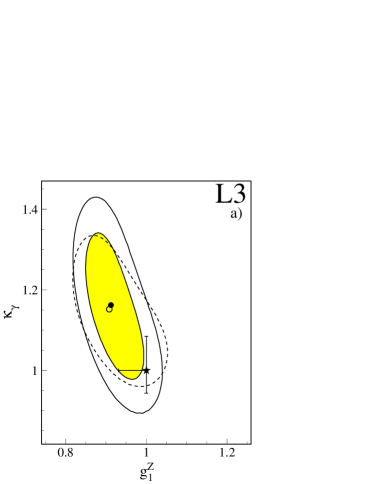
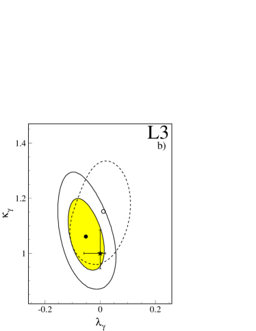
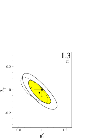
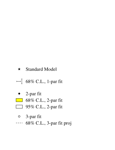
Multi-parameter fits of TGC’s allow a model-independent interpretation of the data. Fits to two of the couplings , and , keeping the third coupling fixed at its Standard Model value, are performed, as well as a simultaneous fit to all these couplings. In each case the constraints and are imposed. The results of these multi-parameter fits are reported in Table 5. The contour curves of 68% and 95% confidence level for the two-parameter fits are shown in Figure 6. They correspond to a change in the negative log-likelihood with respect to its minimum of and , respectively. Contours derived from three-parameter fits are also shown. They are obtained requiring a log-likelihood change of , but leaving the third coupling free to vary in the fit. The comparison of the results derived from fits of different dimensionality shows good agreement.
If the W boson were an extended object, \eg an ellipsoid of rotation with longitudinal radius and transverse radius , its size and shape would be related to the TGCs by [45] and [46], where is the mass of the W boson. The measurements show no evidence for the W boson to be an extended object:
| (4) | |||||
| (5) |
with a correlation coefficient of .
In conclusion, TGC’s are measured with an accuracy of a few percent. All single- and multi-parameter TGC results show good agreement with the Standard Model expectation and confirm the existence of self-couplings among the electroweak gauge bosons.
10
References
- [1] S. L. Glashow, \NP22 (1961) 579; S. Weinberg, \PRL19 (1967) 1264; A. Salam, in Elementary Particle Theory, ed. N. Svartholm, Stockholm, Almquist and Wiksell (1968), 367
- [2] F. Boudjema \etal, in Physics at LEP 2, Report CERN 96-01 (1996), eds. G. Altarelli, T. Sjöstrand, F. Zwirner, Vol. 1, p. 207
- [3] K. Hagiwara \etal, Nucl. Phys. B 282 (1987) 253
- [4] K. Gaemers and G. Gounaris, Z. Phys. C 1 (1979) 259; M. Bilenky \etal, Nucl. Phys. B 409 (1993) 22; Nucl. Phys. B 419 (1994) 240; I. Kuss and D. Schildknecht, Phys. Lett. B 383 (1996) 470
- [5] G. Gounaris \etal, in Physics at LEP 2, Report CERN 96-01 (1996), eds. G. Altarelli, T. Sjöstrand, F. Zwirner, Vol. 1, p. 525
- [6] L3 Collab., M. Acciarri \etal, Phys. Lett. B 467 (1999) 171
- [7] L3 Collab., P. Achard \etal, Phys. Lett. B 547 (2002) 151
- [8] L3 Collab., P. Achard et al., Single- and Multi-Photon Events with Missing Energy in e+e- Collisions at LEP, Preprint CERN-EP-2003-068 (2003)
- [9] UA2 Collab., J. Alitti \etal, Phys. Lett. B 277 (1992) 194; CDF Collab., F. Abe \etal, Phys. Rev. Lett. 74 (1995) 1936; Phys. Rev. Lett. 75 (1995) 1017; Phys. Rev. Lett. 78 (1997) 4536; DØ Collab., S. Abachi \etal, Phys. Rev. Lett. 78 (1997) 3634; Phys. Rev. D 56 (1997) 6742; B. Abbott \etal, Phys. Rev. D 58 (1998) 031102; Phys. Rev. D 58 (1998) 051101; Phys. Rev. D 60 (1999) 072002; Phys. Rev. D 62 (2000) 052005
- [10] ALEPH Collab., R. Barate \etal, Phys. Lett. B 422 (1998) 369; Phys. Lett. B 445 (1998) 239; Phys. Lett. B 462 (1999) 389; Eur. Phys. J. C 21 (2001) 423; DELPHI Collab., P. Abreu \etal, Phys. Lett. B 397 (1997) 158; Phys. Lett. B 423 (1998) 194; Phys. Lett. B 459 (1999) 382; Phys. Lett. B 502 (2001) 9; OPAL Collab., K. Ackerstaff \etal, Phys. Lett. B 397 (1997) 147; Eur. Phys. J. C 2 (1998) 597; G. Abbiendi \etal, Eur. Phys. J. C 8 (1999) 191; Eur. Phys. J. C 19 (2001) 1; CERN-EP-2003-042, submitted to Eur. Phys. J., hep-ex/0308067
- [11] L3 Collab., B. Adeva \etal, Nucl. Instr. Meth. A 289 (1990) 35; J.A. Bakken \etal, Nucl. Instr. Meth. A 275 (1989) 81; O. Adriani \etal, Nucl. Instr. Meth. A 302 (1991) 53; B. Adeva \etal, Nucl. Instr. Meth. A 323 (1992) 109; K. Deiters \etal, Nucl. Instr. Meth. A 323 (1992) 162; M. Chemarin \etal, Nucl. Instr. Meth. A 349 (1994) 345; M. Acciarri \etal, Nucl. Instr. Meth. A 351 (1994) 300; G. Basti \etal, Nucl. Instr. Meth. A 374 (1996) 293; A. Adam \etal, Nucl. Instr. Meth. A 383 (1996) 342; O. Adriani \etal, Phys. Rep. 236 (1993) 1
-
[12]
KandY runs concurrently KORALW version 1.51 and YFSWW version 1.16.
S. Jadach \etal, \CPC140 (2001) 475 - [13] EXCALIBUR version 1.11 is used. F.A. Berends, R. Kleiss and R. Pittau, Comp. Phys. Comm. 85 (1995) 437
- [14] PYTHIA version 6.203 is used. T. Sjöstrand \etal, Comp. Phys. Comm. 135 (2001) 238
- [15] KK2f version 4.14 and 4.19 are used. S. Jadach, B.F.L. Ward and Z. Wa̧s, Comp. Phys. Comm. 130 (2000) 260; S. Jadach, B.F.L. Ward and Z. Wa̧s, \PRD 63 (2001) 113009
- [16] BHAGENE3 Monte Carlo. J.H. Field, \PLB 323 (1994) 432; J.H. Field and T. Riemann, \CPC94 (1996) 53
- [17] BHWIDE version 1.01 is used. S. Jadach, W. Placzek, B.F.L. Ward, Phys. Lett. B 390 (1997) 298
- [18] TEEGG Monte Carlo. D. Karlen, \NP B 289 (1987) 23
- [19] DIAG36 Monte Carlo. F.A. Berends, P.H. Daverfeldt and R. Kleiss, \NPB 253 (1985) 441
- [20] PHOJET version 1.05 is used. R. Engel, \ZfPC 66 (1995) 203; R. Engel and J. Ranft, \PRD 54 (1996) 4244
- [21] KORALW version 1.51 us used. M. Skrzypek \etal, Comp. Phys. Comm. 94 (1996) 216; Phys. Lett. B 372 (1996) 289; S. Jadach \etal, Comp. Phys. Comm. 119 (1999) 272
- [22] W. Beenakker, F.A. Berends and A.P. Chapovsky, Nucl. Phys. B 548 (1999) 3
- [23] YFSWW version 1.14 is used. S. Jadach \etal, Phys. Rev. D 54 (1996) 5434; Phys. Lett. B 417 (1998) 326; Phys. Rev. D 61 (2000) 113010; Phys. Rev. D 65 (2002) 093010
- [24] GEANT version 3.15 is used. R. Brun \etal, preprint CERN DD/EE/84-1 (1985), revised 1987. The GHEISHA program (H. Fesefeldt, RWTH Aachen Report PITHA 85/02, 1985) is used to simulate hadronic interactions
- [25] L3 Collab., M. Acciarri \etal, Phys. Lett. B 496 (2000) 19
- [26] L3 Collab., P. Achard \etal, Measurement of the Cross Section of W Pair-Production at LEP, in preparation
- [27] S. Villa Measurement of the Triple Gauge Couplings of the W Boson at LEP2, Ph.D. thesis, Northeastern University, Boston, 2000
- [28] M. Dierckxsens, Measurement of Triple Gauge-Boson Couplings in Collisions at LEP, Ph.D. thesis, University of Nijmegen, 2004
- [29] G.K. Fanourakis, D. Fassouliotis and S.E. Tzamarias, Nucl. Instr. and Meth. A 414 (1998) 399; L3 Collab., P. Achard \etal, Search for Triple Neutral Gauge Boson Couplings in the Process at LEP, in preparation
- [30] A. Jacholkowska, J. Kalinowski and Z. Wa̧s, Comp. Phys. Comm. 124 (2000) 238
- [31] B.F.L. Ward, S. Jadach and Z. Wa̧s, Nucl. Phys. Proc. Suppl. 116 (2003) 73
- [32] A. Jacholkowska, J. Kalinowski and Z. Wa̧s, Eur. Phys. J. C 6 (1999) 485
- [33] M.W. Grünewald \etal, in Reports of the Working Groups on Precision Calculations for LEP2 Physics, Report CERN 2000-009 (2000), eds. S. Jadach, G. Passarino and R. Pittau, p. 1
- [34] RacoonWW Monte Carlo. A. Denner \etal, \PLB 475 (2000) 127; Nucl. Phys. B 587 (2000) 67
- [35] R. Brunelière \etal, Phys. Lett. B 533 (2002) 75
- [36] K. Hagiwara \etal, Phys. Rev. D 66 (2002) 1
- [37] HERWIG version 6.202 is used. G. Marchesini \etal, Comp. Phys. Comm. 67 (1992) 465; G. Corcella \etal, JHEP 0101:010,2001
- [38] ARIADNE version 4.12 is used. L. Lönnblad, Comp. Phys. Comm. 71 (1992) 15
- [39] G. Gustafson, U. Petterson and P.M. Zerwas, Phys. Lett. B 209 (1988) 90; T. Sjöstrand and V.A. Khoze, Z. Phys. C 62 (1994) 281, Phys. Rev. Lett. 72 (1994) 28; G. Gustafson and J. Häkkinen, Z. Phys. C 64 (1994) 659; C. Friberg, G. Gustafson and J. Häkkinen, Nucl. Phys. B 490 (1997) 289; B.R. Webber, J. Phys. G 24 (1998) 287
- [40] L. Lönnblad and T. Sjöstrand, Phys. Lett. B 351 (1995) 293; A. Ballestrero \etal in Physics at LEP 2, Report CERN 96-01 (1996), eds. G. Altarelli, T. Sjöstrand, F. Zwirner, Vol. 1, p. 141; V. Kartvelishvili, R. Kvatadze and R. Møller, Phys. Lett. B 408 (1997) 331; S. Jadach and K. Zalewski, Acta Phys. Pol. B 28 (1997) 1363; K. Fiałkowski and R. Wit, Acta Phys. Pol. B 28 (1997) 2039; K. Fiałkowski, R. Wit and J. Wosiek, Phys. Rev. D 58 (1998) 094013
- [41] L. Lönnblad, Z. Phys. C 70 (1996) 107
- [42] T. Sjöstrand and V. Khoze, Z. Phys. C 62 (1994) 281; V. Khoze and T. Sjöstrand, Eur. Phys. J. C 6 (1999) 271
- [43] L3 Collab., P. Achard \etal, Phys. Lett. B 561 (2003) 202
- [44] L. Lönnblad and T. Sjöstrand, Eur. Phys. J. C 2 (1998) 165
- [45] S.J. Brodsky and S.D. Drell, Phys. Rev. D 22 (1980) 2236
-
[46]
H. Frauenfelder and E.M. Henley, Subatomic physics, Englewood Cliffs, New
Jersey (1974)
The L3 Collaboration:
P.Achard,20 O.Adriani,17 M.Aguilar-Benitez,24 J.Alcaraz,24 G.Alemanni,22 J.Allaby,18 A.Aloisio,28 M.G.Alviggi,28 H.Anderhub,46 V.P.Andreev,6,33 F.Anselmo,8 A.Arefiev,27 T.Azemoon,3 T.Aziz,9 P.Bagnaia,38 A.Bajo,24 G.Baksay,25 L.Baksay,25 S.V.Baldew,2 S.Banerjee,9 Sw.Banerjee,4 A.Barczyk,46,44 R.Barillère,18 P.Bartalini,22 M.Basile,8 N.Batalova,43 R.Battiston,32 A.Bay,22 F.Becattini,17 U.Becker,13 F.Behner,46 L.Bellucci,17 R.Berbeco,3 J.Berdugo,24 P.Berges,13 B.Bertucci,32 B.L.Betev,46 M.Biasini,32 M.Biglietti,28 A.Biland,46 J.J.Blaising,4 S.C.Blyth,34 G.J.Bobbink,2 A.Böhm,1 L.Boldizsar,12 B.Borgia,38 S.Bottai,17 D.Bourilkov,46 M.Bourquin,20 S.Braccini,20 J.G.Branson,40 F.Brochu,4 J.D.Burger,13 W.J.Burger,32 X.D.Cai,13 M.Capell,13 G.Cara Romeo,8 G.Carlino,28 A.Cartacci,17 J.Casaus,24 F.Cavallari,38 N.Cavallo,35 C.Cecchi,32 M.Cerrada,24 M.Chamizo,20 Y.H.Chang,48 M.Chemarin,23 A.Chen,48 G.Chen,7 G.M.Chen,7 H.F.Chen,21 H.S.Chen,7 G.Chiefari,28 L.Cifarelli,39 F.Cindolo,8 I.Clare,13 R.Clare,37 G.Coignet,4 N.Colino,24 S.Costantini,38 B.de la Cruz,24 S.Cucciarelli,32 J.A.van Dalen,30 R.de Asmundis,28 P.Déglon,20 J.Debreczeni,12 A.Degré,4 K.Dehmelt,25 K.Deiters,44 D.della Volpe,28 E.Delmeire,20 P.Denes,36 F.DeNotaristefani,38 A.De Salvo,46 M.Diemoz,38 M.Dierckxsens,2 C.Dionisi,38 M.Dittmar,46 A.Doria,28 M.T.Dova,10,♯ D.Duchesneau,4 M.Duda,1 B.Echenard,20 A.Eline,18 A.El Hage,1 H.El Mamouni,23 A.Engler,34 F.J.Eppling,13 P.Extermann,20 M.A.Falagan,24 S.Falciano,38 A.Favara,31 J.Fay,23 O.Fedin,33 M.Felcini,46 T.Ferguson,34 H.Fesefeldt,1 E.Fiandrini,32 J.H.Field,20 F.Filthaut,30 P.H.Fisher,13 W.Fisher,36 I.Fisk,40 G.Forconi,13 K.Freudenreich,46 C.Furetta,26 Yu.Galaktionov,27,13 S.N.Ganguli,9 P.Garcia-Abia,24 M.Gataullin,31 S.Gentile,38 S.Giagu,38 Z.F.Gong,21 G.Grenier,23 O.Grimm,46 M.W.Gruenewald,16 M.Guida,39 R.van Gulik,2 V.K.Gupta,36 A.Gurtu,9 L.J.Gutay,43 D.Haas,5 D.Hatzifotiadou,8 T.Hebbeker,1 A.Hervé,18 J.Hirschfelder,34 H.Hofer,46 M.Hohlmann,25 G.Holzner,46 S.R.Hou,48 Y.Hu,30 B.N.Jin,7 L.W.Jones,3 P.de Jong,2 I.Josa-Mutuberría,24 M.Kaur,14 M.N.Kienzle-Focacci,20 J.K.Kim,42 J.Kirkby,18 W.Kittel,30 A.Klimentov,13,27 A.C.König,30 M.Kopal,43 V.Koutsenko,13,27 M.Kräber,46 R.W.Kraemer,34 A.Krüger,45 A.Kunin,13 P.Ladron de Guevara,24 I.Laktineh,23 G.Landi,17 M.Lebeau,18 A.Lebedev,13 P.Lebrun,23 P.Lecomte,46 P.Lecoq,18 P.Le Coultre,46 J.M.Le Goff,18 R.Leiste,45 M.Levtchenko,26 P.Levtchenko,33 C.Li,21 S.Likhoded,45 C.H.Lin,48 W.T.Lin,48 F.L.Linde,2 L.Lista,28 Z.A.Liu,7 W.Lohmann,45 E.Longo,38 Y.S.Lu,7 C.Luci,38 L.Luminari,38 W.Lustermann,46 W.G.Ma,21 L.Malgeri,20 A.Malinin,27 C.Maña,24 J.Mans,36 J.P.Martin,23 F.Marzano,38 K.Mazumdar,9 R.R.McNeil,6 S.Mele,18,28 L.Merola,28 M.Meschini,17 W.J.Metzger,30 A.Mihul,11 H.Milcent,18 G.Mirabelli,38 J.Mnich,1 G.B.Mohanty,9 G.S.Muanza,23 A.J.M.Muijs,2 B.Musicar,40 M.Musy,38 S.Nagy,15 S.Natale,20 M.Napolitano,28 F.Nessi-Tedaldi,46 H.Newman,31 A.Nisati,38 T.Novak,30 H.Nowak,45 R.Ofierzynski,46 G.Organtini,38 I.Pal,43C.Palomares,24 P.Paolucci,28 R.Paramatti,38 G.Passaleva,17 S.Patricelli,28 T.Paul,10 M.Pauluzzi,32 C.Paus,13 F.Pauss,46 M.Pedace,38 S.Pensotti,26 D.Perret-Gallix,4 B.Petersen,30 D.Piccolo,28 F.Pierella,8 M.Pioppi,32 P.A.Piroué,36 E.Pistolesi,26 V.Plyaskin,27 M.Pohl,20 V.Pojidaev,17 J.Pothier,18 D.Prokofiev,33 J.Quartieri,39 G.Rahal-Callot,46 M.A.Rahaman,9 P.Raics,15 N.Raja,9 R.Ramelli,46 P.G.Rancoita,26 R.Ranieri,17 A.Raspereza,45 P.Razis,29D.Ren,46 M.Rescigno,38 S.Reucroft,10 S.Riemann,45 K.Riles,3 B.P.Roe,3 L.Romero,24 A.Rosca,45 C.Rosemann,1 C.Rosenbleck,1 S.Rosier-Lees,4 S.Roth,1 J.A.Rubio,18 G.Ruggiero,17 H.Rykaczewski,46 A.Sakharov,46 S.Saremi,6 S.Sarkar,38 J.Salicio,18 E.Sanchez,24 C.Schäfer,18 V.Schegelsky,33 H.Schopper,47 D.J.Schotanus,30 C.Sciacca,28 L.Servoli,32 S.Shevchenko,31 N.Shivarov,41 V.Shoutko,13 E.Shumilov,27 A.Shvorob,31 D.Son,42 C.Souga,23 P.Spillantini,17 M.Steuer,13 D.P.Stickland,36 B.Stoyanov,41 A.Straessner,20 K.Sudhakar,9 G.Sultanov,41 L.Z.Sun,21 S.Sushkov,1 H.Suter,46 J.D.Swain,10 Z.Szillasi,25,¶ X.W.Tang,7 P.Tarjan,15 L.Tauscher,5 L.Taylor,10 B.Tellili,23 D.Teyssier,23 C.Timmermans,30 Samuel C.C.Ting,13 S.M.Ting,13 S.C.Tonwar,9
J.Tóth,12 C.Tully,36 K.L.Tung,7J.Ulbricht,46 E.Valente,38 R.T.Van de Walle,30 R.Vasquez,43 V.Veszpremi,25 G.Vesztergombi,12 I.Vetlitsky,27 D.Vicinanza,39 G.Viertel,46 S.Villa,37 M.Vivargent,4 S.Vlachos,5 I.Vodopianov,25 H.Vogel,34 H.Vogt,45 I.Vorobiev,34,27 A.A.Vorobyov,33 M.Wadhwa,5 Q.Wang30 X.L.Wang,21 Z.M.Wang,21 M.Weber,18 H.Wilkens,30 S.Wynhoff,36 L.Xia,31 Z.Z.Xu,21 J.Yamamoto,3 B.Z.Yang,21 C.G.Yang,7 H.J.Yang,3 M.Yang,7 S.C.Yeh,49 An.Zalite,33 Yu.Zalite,33 Z.P.Zhang,21 J.Zhao,21 G.Y.Zhu,7 R.Y.Zhu,31 H.L.Zhuang,7 A.Zichichi,8,18,19 B.Zimmermann,46 M.Zöller.1
-
1
III. Physikalisches Institut, RWTH, D-52056 Aachen, Germany§
-
2
National Institute for High Energy Physics, NIKHEF, and University of Amsterdam, NL-1009 DB Amsterdam, The Netherlands
-
3
University of Michigan, Ann Arbor, MI 48109, USA
-
4
Laboratoire d’Annecy-le-Vieux de Physique des Particules, LAPP,IN2P3-CNRS, BP 110, F-74941 Annecy-le-Vieux CEDEX, France
-
5
Institute of Physics, University of Basel, CH-4056 Basel, Switzerland
-
6
Louisiana State University, Baton Rouge, LA 70803, USA
-
7
Institute of High Energy Physics, IHEP, 100039 Beijing, China△
-
8
University of Bologna and INFN-Sezione di Bologna, I-40126 Bologna, Italy
-
9
Tata Institute of Fundamental Research, Mumbai (Bombay) 400 005, India
-
10
Northeastern University, Boston, MA 02115, USA
-
11
Institute of Atomic Physics and University of Bucharest, R-76900 Bucharest, Romania
-
12
Central Research Institute for Physics of the Hungarian Academy of Sciences, H-1525 Budapest 114, Hungary‡
-
13
Massachusetts Institute of Technology, Cambridge, MA 02139, USA
-
14
Panjab University, Chandigarh 160 014, India.
-
15
KLTE-ATOMKI, H-4010 Debrecen, Hungary¶
-
16
Department of Experimental Physics, University College Dublin, Belfield, Dublin 4, Ireland
-
17
INFN Sezione di Firenze and University of Florence, I-50125 Florence, Italy
-
18
European Laboratory for Particle Physics, CERN, CH-1211 Geneva 23, Switzerland
-
19
World Laboratory, FBLJA Project, CH-1211 Geneva 23, Switzerland
-
20
University of Geneva, CH-1211 Geneva 4, Switzerland
-
21
Chinese University of Science and Technology, USTC, Hefei, Anhui 230 029, China△
-
22
University of Lausanne, CH-1015 Lausanne, Switzerland
-
23
Institut de Physique Nucléaire de Lyon, IN2P3-CNRS,Université Claude Bernard, F-69622 Villeurbanne, France
-
24
Centro de Investigaciones Energéticas, Medioambientales y Tecnológicas, CIEMAT, E-28040 Madrid, Spain
-
25
Florida Institute of Technology, Melbourne, FL 32901, USA
-
26
INFN-Sezione di Milano, I-20133 Milan, Italy
-
27
Institute of Theoretical and Experimental Physics, ITEP, Moscow, Russia
-
28
INFN-Sezione di Napoli and University of Naples, I-80125 Naples, Italy
-
29
Department of Physics, University of Cyprus, Nicosia, Cyprus
-
30
University of Nijmegen and NIKHEF, NL-6525 ED Nijmegen, The Netherlands
-
31
California Institute of Technology, Pasadena, CA 91125, USA
-
32
INFN-Sezione di Perugia and Università Degli Studi di Perugia, I-06100 Perugia, Italy
-
33
Nuclear Physics Institute, St. Petersburg, Russia
-
34
Carnegie Mellon University, Pittsburgh, PA 15213, USA
-
35
INFN-Sezione di Napoli and University of Potenza, I-85100 Potenza, Italy
-
36
Princeton University, Princeton, NJ 08544, USA
-
37
University of Californa, Riverside, CA 92521, USA
-
38
INFN-Sezione di Roma and University of Rome, “La Sapienza”, I-00185 Rome, Italy
-
39
University and INFN, Salerno, I-84100 Salerno, Italy
-
40
University of California, San Diego, CA 92093, USA
-
41
Bulgarian Academy of Sciences, Central Lab. of Mechatronics and Instrumentation, BU-1113 Sofia, Bulgaria
-
42
The Center for High Energy Physics, Kyungpook National University, 702-701 Taegu, Republic of Korea
-
43
Purdue University, West Lafayette, IN 47907, USA
-
44
Paul Scherrer Institut, PSI, CH-5232 Villigen, Switzerland
-
45
DESY, D-15738 Zeuthen, Germany
-
46
Eidgenössische Technische Hochschule, ETH Zürich, CH-8093 Zürich, Switzerland
-
47
University of Hamburg, D-22761 Hamburg, Germany
-
48
National Central University, Chung-Li, Taiwan, China
-
49
Department of Physics, National Tsing Hua University, Taiwan, China
-
§
Supported by the German Bundesministerium für Bildung, Wissenschaft, Forschung und Technologie
-
‡
Supported by the Hungarian OTKA fund under contract numbers T019181, F023259 and T037350.
-
¶
Also supported by the Hungarian OTKA fund under contract number T026178.
-
Supported also by the Comisión Interministerial de Ciencia y Tecnología.
-
Also supported by CONICET and Universidad Nacional de La Plata, CC 67, 1900 La Plata, Argentina.
-
Supported by the National Natural Science Foundation of China.
-
1
| 188.6 | 191.6 | 195.5 | 199.6 | 201.8 | 204.8 | 206.5 | 208.0 | |
| 176.8 | 29.8 | 84.1 | 83.3 | 37.1 | 79.0 | 130.5 | 8.6 |
| Process | ||
|---|---|---|
| Source | Systematic uncertainty | |||||
|---|---|---|---|---|---|---|
| of uncertainty | ||||||
| Uncertainty on | 0.003 | 0.018 | 0.006 | 0.03 | 0.009 | 0.014 |
| corrections on | 0.004 | 0.004 | 0.003 | 0.01 | 0.011 | 0.007 |
| Background modelling | 0.005 | 0.019 | 0.006 | 0.02 | 0.009 | 0.014 |
| Jet charge confusion | 0.001 | 0.006 | 0.002 | 0.002 | 0.005 | |
| Lepton charge confusion | 0.003 | 0.013 | 0.007 | 0.005 | 0.009 | |
| Jet and lepton measurement | 0.001 | 0.003 | 0.002 | 0.01 | 0.002 | 0.004 |
| Monte Carlo statistics | 0.012 | 0.010 | 0.014 | 0.02 | 0.016 | 0.007 |
| ISR and FSR | 0.001 | 0.016 | 0.001 | 0.01 | 0.002 | 0.002 |
| W mass and width | 0.001 | 0.005 | 0.002 | 0.01 | 0.002 | 0.004 |
| Fragmentation | 0.003 | 0.002 | 0.001 | 0.02 | 0.004 | 0.001 |
| Bose Einstein correlations | 0.001 | 0.001 | 0.001 | 0.001 | 0.003 | |
| Colour reconnection | 0.001 | 0.004 | 0.001 | 0.02 | 0.002 | 0.003 |
| Total systematic uncertainty | 0.015 | 0.039 | 0.017 | 0.05 | 0.024 | 0.023 |
| Coupling | |||
|---|---|---|---|
| 189–209 | |||
| We 161–209 | |||
| WW 161–209 | |||
| All channels combined | |||
| Standard Model value | 1.0 | 1.0 | 0.0 |
| Coupling | |||
| WW 189-209 | |||
| Standard Model value | 0.0 | 1.0 | 0.0 |
| Fit | Standard | Results | correlation coeffs. | |||
| parameter | Model | (68% CL) | (95% CL) | |||
| two-parameter fits | ||||||
| 1.0 | ||||||
| 1.0 | ||||||
| 1.0 | ||||||
| 0.0 | ||||||
| 1.0 | ||||||
| 0.0 | ||||||
| three-parameter fit | ||||||
| 1.0 | ||||||
| 1.0 | ||||||
| 0.0 | ||||||