A Proposal for a Near Detector Experiment on the Booster Neutrino Beamline:
FINeSSE: Fermilab Intense Neutrino Scattering Scintillator Experiment

L. Bugel, J. M. Conrad, J. M. Link, M. Shaevitz, L. Wang, G. P. Zeller
Columbia University, Nevis Labs, Irvington, NY 10533
S. Brice, B. T. Fleming^∗, D. Finley, R.  Stefanski
Fermi National Accelerator Laboratory, Batavia, IL 60510
J. C. Peng
University of Illinois at Urbana-Champaign, Urbana, IL 61801
J. Doskow, C. Horowitz, T. Katori, H. O. Meyer, P. Ockerse, R. Tayloe^∗, G. Visser
Indiana University, Bloomington, IN 47408
C. Green, G. T. Garvey, W. C. Louis, G. McGregor, R. Van de Water
Los Alamos National Laboratory, Los Alamos, NM 87545
R. Imlay, W. Metcalf, M. Sung, M. O. Wascko
Louisiana State University, Baton Rouge, LA 70803
V. Papavassiliou
New Mexico State University, Las Cruces, NM 88003
L. Lu
University of Virginia, Charlottesville, VA 22901

ABSTRACT
FINeSSE: Fermilab Intense Neutrino Scattering Scintillator Experiment

Understanding the quark and gluon substructure of the nucleon has been a prime goal of both nuclear and particle physics for more than thirty years and has led to much of the progress in strong interaction physics. Still the flavor dependence of the nucleon’s spin is a significant fundamental question that is not understood. Experiments measuring the spin content of the nucleon have reported conflicting results on the amount of nucleon spin carried by strange quarks. Quasi-elastic neutrino scattering, observed using a novel detection technique, provides a theoretically clean measure of this quantity.

The optimum neutrino beam energy needed to measure the strange spin of the nucleon is 1 GeV. This is also an ideal energy to search for neutrino oscillations at high $\Delta m^{2}$ in an astrophysically interesting region. Models of the r-process in supernovae which include high-mass sterile neutrinos may explain the abundance of neutron-rich heavy metals in the universe. These high-mass sterile neutrinos are outside the sensitivity region of any previous neutrino oscillation experiments.

The Booster neutrino beamline at Fermilab provides the world’s highest intensity neutrino beam in the 0.5-1.0 GeV energy range, a range ideal for both of these measurements. A small detector located upstream of the MiniBooNE detector, 100 m from the recently commissioned Booster neutrino source, could definitively measure the strange quark contribution to the nucleon spin. This detector, in conjunction with the MiniBooNE detector, could also investigate $\nu_{\mu}$ disappearance in a currently unexplored, cosmologically interesting region.

Chapter 1 Introduction

The Fermilab Intense Neutrino Scattering Scintillator Experiment (“FINeSSE”) is designed to measure the strange quark contribution to the spin of the proton, and to search, in conjunction with the MiniBooNE experiment, for $\nu_{\mu}$ disappearance. These measurements will employ a novel detection technique, and will examine a kinematic region inaccessible to any existing or presently-planned experiment. FINeSSE will be located 100 m from the Booster neutrino beamline production target, and 441 m upstream of the currently-running MiniBooNE experiment. The low energy Booster neutrino beam is crucial to achieving this experiment’s goals; they can only be realized on this Fermilab beamline. The number of protons on target (POT) needed to reach the FINeSSE physics goals is 6$\times 10^{20}$, attainable in two years of running. The detector is designed to resolve both short, low energy proton tracks, and longer muon tracks from $\nu N$ interactions. The FINeSSE detector will cost $2.25M ($2.8M with contingency); the FINeSSE Detector enclosure, $800K ($1.6M with contingency, escalation, and EDIA).

1.1 Outline

This proposal sets forth the experiment’s goals, design, costs, and schedule in the following sections:

• Chapter 2 provides the physics motivation for FINeSSE;

• Chapter 3 describes the flux and event rate at FINeSSE produced by the Booster neutrino beamline;

• Chapter 4 details the detector design, construction, and installation, as well as the readout and trigger systems;

• Chapter 5 examines event kinematics, efficiencies, and backgrounds for the FINeSSE physics measurements;

• Chapter 6 points out additional physics measurements the FINeSSE experiment can perform;

• Chapter 7 provides a breakdown of costs for the detector, the electronics, and an enclosure for both, as well as a timeline to first beam in mid-2006.

1.2 FINeSSE Physics, Detector, and Neutrino Beam

The fundamental question of the flavor dependence of the spin of the proton is not understood. The still unresolved “spin crisis” [2] points to the fact that the proton’s spin is not carried, as was expected, by the valence quarks. How much is carried by the light quark sea has been the subject of much controversy. In addition, measurements of the spin carried by the strange quarks in the nucleon have been plagued by model assumptions and experimental limitations. The FINeSSE experiment will measure the proton’s strange spin, $\Delta s$, avoiding the pitfalls of previous measurements; our approach will be described in detail in Chapter 2.

FINeSSE, in conjunction with the MiniBooNE experiment, is sensitive to $\nu_{\mu}$ disappearance in an as-yet unexplored, astrophysically interesting region. Incorporating oscillations to  1 eV sterile neutrinos into the r-process in supernovae can explain the abundance of neutron-rich heavy metals in the universe [3]. Oscillations between these sterile neutrinos and muon neutrinos are expected over short baselines for neutrino energies around 1 GeV. The combination of FINeSSE and MiniBooNE, functioning as near and far detector, enables a $\nu_{\mu}$ disappearance search sensitive to these oscillations. This sensitivity exceeds that of any existing or planned experiment, and permits exploration of the full allowed 3+1 region.

The physics goals of FINeSSE can be achieved using a novel, relatively small, tracking detector placed 100 m from the neutrino production target on the Booster neutrino beam line (Fig. 1.1). The detector is comprised of two subdetectors. The upstream Vertex Detector is a highly-segmented, liquid scintillator “bubble chamber” that tracks particle interactions via scintillation light read out on a grid of Wavelength Shifting (WLS) fiber strung throughout the volume. The Muon Rangestack downstream of the Vertex Detector ranges out high energy muons produced in neutrino interactions.

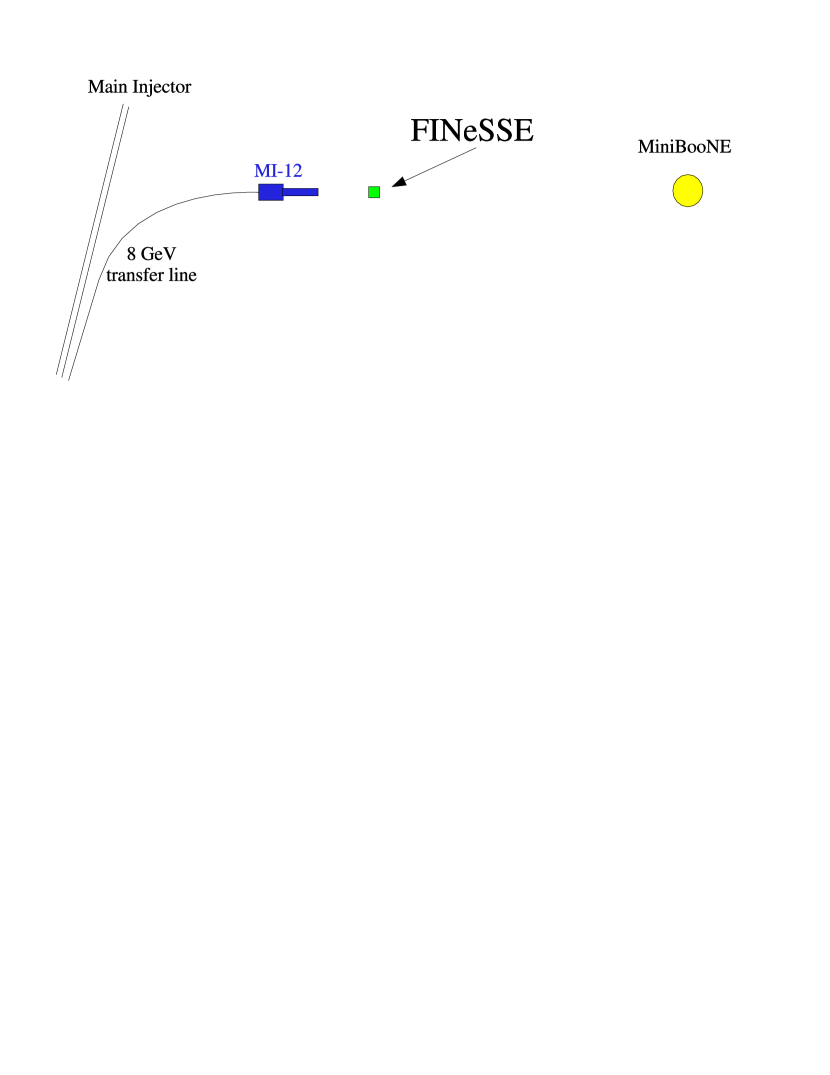
Figure 1.1: Proposed FINeSSE location with respect to the existing neutrino target building (MI-12) and MiniBooNE detector. North is to the right in this drawing.

The Booster neutrino beam provides an intense source of muon neutrinos (with a small background of electron neutrinos) in the energy range of 0.5-1.5 GeV and a mean energy of $\sim$ 700 MeV. This spectrum is ideal for the $\nu p$ elastic scattering measurement as well as for the $\nu_{\mu}$ disappearance search. Using the currently estimated MiniBooNE neutrino flux [4], and assuming $3.0\times 10^{20}$ protons on target per year [5], there would be approximately 360k neutrino scattering events in a detector of 9 ton active volume during the FINeSSE run of 2 years. This would provide a neutrino event sample of unprecedented size in this energy range.

1.3 The FINeSSE Collaboration

FINeSSE is currently a collaboration of 29 scientists from six universities and two national laboratories. Once approved, the collaboration is expected to grow. Both university groups and national labs have already incorporated post-docs, graduate students, undergraduates, and a high school teacher into FINeSSE physics projects. FINeSSE has organized an executive committee comprised of senior scientists from each group to oversee the project. The collaboration is diverse yet balanced in a number of ways:

• Collaborators are drawn from both the nuclear and particle physics communities. This will help the collaboration to attain its physics goals, which span both of these communities, and will encourage cross-disciplinary interactions between nuclear and particle physicists, as well.

• FINeSSE is comprised of both MiniBooNE and non-MiniBooNE scientists. This balance helps to ensure a good understanding of a neutrino beam already well studied by MiniBooNE, and at the same time bring in new ideas and perspectives on physics with this beam.

• FINeSSE scientists carry with them a broad spectrum of experience. The new perspectives brought by the FINeSSE spokespeople are tempered by a well-seasoned executive committee comprised of experienced scientists with, again, both nuclear and particle physics backgrounds.

FINeSSE’s diversity in background and experience are already a great asset to its physics program, and will help to sustain it throughout its physics run.

1.4 FINeSSE as part of the Fermilab program

FINeSSE brings timely and important physics to the Fermilab program. In addition, FINeSSE takes advantage of the investment Fermilab has already made in the Booster neutrino beamline, provides an excellent training ground for young Fermilab scientists, and already actively contributes to the growing Fermilab neutrino program.

To achieve its physics goals, FINeSSE requires $6.0\times 10^{20}$ total protons on target, received over the course of a two year run on the Booster neutrino beamline. This is within the Booster’s capability in the era of NuMI and Run II running, as described in Chapter 3 and Reference [5]. It also takes advantage of a running beam, and another running experiment, adding value to already committed resources.

FINeSSE is a small, focused collaboration. Such groups are proven training grounds for graduate students and post-docs, vital to the future of Fermilab and of high energy physics. It is on such small-scale experiments that young scientists are guaranteed to get their hands on almost every aspect of design, construction, data taking, and data analysis.

In summary, FINeSSE represents an important addition to Fermilab’s program: it provides an extraordinary opportunity for physicists from a number of subfields and a variety of levels of experience to work together; it makes advantageous use of an existing beamline; it increases the physics reach of an existing experiment; and it uses a novel detection technique to address significant and interesting physics.

1.5 Requests to the PAC

Please consider the following specific requests with respect to approval and funding for FINeSSE:

• Grant this experiment “stage 0” or “stage 1” approval at this time (approval pending response to any outstanding questions). This will allow us to submit an NSF proposal by a January 2004 deadline.

• Recommend to the Fermilab directorate to support FINeSSE for the first stages of detector enclosure design work.

• Recommend to the Fermilab directorate to provide FINeSSE with office and lab space.

Chapter 2 Physics Motivation

Two physics measurements form the foundation of the FINeSSE program: the measurement of the strange spin of the proton, $\Delta s$; and the search for $\nu_{\mu}$ disappearance in an astrophysically interesting region. Both topics are compelling, and can only be addressed with the Booster neutrino beam design. Along with these studies, a complement of other measurements and searches are open to FINeSSE. These other physics projects are addressed in Chapter 6. In this chapter we concentrate on the two main physics goals, which make FINeSSE unique.

2.1 Strange Quark Contribution to Nucleon Spin

From the time that the composite nature of the proton was discovered, physicists have sought to understand its constituents. The study of nucleon spin has grown into an industry experimentally, and opened new frontiers theoretically. Deep Inelastic Scattering (DIS) measurements with polarized beams and/or targets have given us a direct measurement of the spins carried by the quarks in the nucleon. A central mystery has unfolded: in the nucleon, if the $u$ and $d$ valence quarks carry approximately equal and opposite spins, where lies the remainder?

One key contribution that has eluded a definitive explanation is the spin contribution from strange quarks in the nucleon sea. A large strange quark spin component, extracted from recent measurements [6], would be of intense theoretical interest, since it would require significant changes to current assumptions. Is this large value of the strange spin due to chiral solitons [7], a misinterpretation of the large gluon contributions coming from the QCD axial anomaly [8, 9], or incorrect assumptions of SU(3) symmetry [10]? In addition, an understanding of the nucleon spin structure is a key input to dark matter searches, since the couplings of supersymmetric particles and axions to dark matter depend upon the components of the spin.

It has been known for some time that low energy (and low $Q^{2}$) neutrino measurements are the only theoretically robust technique (as robust as, e.g., the Bjorken sum rule) for isolating the strange quark contribution. New low energy, intense neutrino beams now make it possible to take greater advantage of this method. The FINeSSE experiment, using these newly-available beams along with a novel detection technique, will resolve the presently murky experimental picture, providing results which are interesting both to particle physics and astrophysics.

FINeSSE will measure $\Delta s$ by examining neutral current neutrino-proton scattering; the rate of this process is sensitive to any contributions from strange quarks (both $s$ and $\bar{s}$) to the nucleon spin. Specifically, $\Delta s$ is extracted from the ratio of neutral current neutrino-proton ($\nu p\rightarrow\nu p$) scattering to charged current neutrino-neutron ($\nu n\rightarrow\mu^{-}p$) scattering. The measurement will be made at low momentum transfer ($Q^{2}\approx 0.2$ GeV²), in order to unambiguously extract $\Delta s$ from the axial form factor, $G_{A}$. FINeSSE will improve on the latest measurement of neutral current neutrino-proton scattering (BNL 734) by measuring this process at a lower-$Q^{2}$, with more events, less background, and lower systematic uncertainty.

In the following sections, we describe some of the previous and current experiments relevant to the question of strange quarks in the nucleon. We then describe why neutral current neutrino-nucleon elastic scattering is sensitive to the strange-quark contributions to the nucleon spin. We conclude with a summary of the sensitivity of FINeSSE to $\Delta s$ (detailed more completely in Chapter 5).

2.1.1 Experimental Results: Strange Quarks in the Nucleon

The role that strange quarks play in determining the properties of the nucleon is an area of much experimental and theoretical interest, and is not well understood. Deep inelastic scattering of neutrinos on nucleons indicate that strange quarks constitute a substantial fraction (20%) of the nucleon sea [11]. Nevertheless, the latest results from parity-violating (PV) electron scattering show that the contribution of strange quarks to the charge and magnetic moment of the nucleon is consistent with zero [12, 13]. However, results from DIS of polarized charged leptons indicate non-zero contributions of strange quarks to the nucleon spin. In the sections that follow, we describe the some of the experimental and theoretical issues which FINeSSE will help to address.

Parity-Violating Electron Scattering

There is a large and continuing effort to investigate the nucleon structure via Parity-Violating (PV) electron scattering. Electron scattering is sensitive to the strange (and anti-strange) quark contributions to the nucleon charge and magnetic moment distributions. The recently-completed MIT/Bates SAMPLE experiment [12] measured the strange-magnetic form factor, $G_{M}^{s}$, at a momentum transfer $Q^{2}=0.1$ GeV², to be consistent with zero (albeit with large errors). The ongoing Jefferson Lab HAPPEX experiment [13] measures a PV scattering asymmetry sensitive to a combination of the strange-electric and strange-magnetic form factors ($G_{E}^{s}$ and $G_{M}^{s}$) at $Q^{2}=0.48$ GeV². This combination is also consistent with no strange-quark effects in the nucleon. HAPPEX continues to search, and will make a measurement at lower $Q^{2}(=0.1$ GeV²) on a helium target in the near future [14].

Upcoming PV electron experiments looking for strange quark effects are the PVA4 experiment [15] at Mainz, which will measure a combination of $G_{E}^{s}$ and $G_{M}^{s}$ at $Q^{2}$ from 0.1 - 0.48 GeV²; and the G0 experiment [16], which will cover a large $Q^{2}$ (0.1 - 1.0 eV²) range.

There is a large effort to look for strange quark effects via PV electron scattering. Unfortunately, these measurements are not sensitive to the strange axial vector form factor ($G_{A}^{s}$, related to the spin structure and $\Delta s$). This is because the parity violating contribution to the axial vector form factor of the nucleon couples via the very small vector form factor of the charged lepton ($1-4\sin\theta_{W}$). As a result, this contribution to the PV asymmetry is dominated by a large PV radiative correction known as the anapole moment [12].

PV electron scattering combined with neutrino scattering would be a powerful approach to the study of strange quark effects in the nucleon. As will be explained below, neutrino scattering is very sensitive to the strange axial-vector form factor $G_{A}^{s}$, and much less so to the strange electric and magnetic form factors $G_{E}^{s}$ and $G_{M}^{s}$. The opposite is true in PV electron scattering. The measurements from FINeSSE could be combined with those from this thorough program of PV electron scattering to obtain accurate knowledge of all three strange form factors $G_{A}^{s}$, $G_{E}^{s}$, and $G_{M}^{s}$ [17].

Polarized Lepton Deep Inelastic Scattering

Results obtained in DIS by polarized leptons from polarized nucleons have been interpreted (from measurements of the polarized structure function, $g_{1}^{p}$) as evidence for a non-zero and negative $\Delta s$. The SMC experiment, e.g., has reported $\Delta s=-0.10\pm 0.05$ [18]. The method of extracting $\Delta s$ from $g_{1}^{p}$, however, has been subject to much debate, due to model-dependent assumptions of $SU(3)$ symmetry [10, 19] and to extrapolation of the spin structure function to $x\rightarrow 0$ [8]. In addition, recent controversial results from HERMES [20] semi-inclusive DIS indicate a zero or small positive value for $\Delta s$ ($\Delta s=+0.03\pm 0.03\pm 0.01$ where the first error is statistical and the second is systematic). It should be noted that the HERMES measurement is only sensitive to $\Delta s$, as opposed to the SMC measurement of $\Delta s+\Delta\bar{s}$ [20]. The errors reported in these current “state-of-the-art” DIS measurements of $\Delta s$ are typically in the range of $0.02-0.05$.

As will be shown in the sections below, the interpretation of neutral current neutrino-nucleon scattering suffers from none of the theoretical uncertainties inherent in the DIS measurements.

Neutral-Current Neutrino Scattering

The best measurement to date of neutral current neutrino scattering is Experiment E734 at Brookhaven National Laboratory (BNL). They measured neutrino-proton ($\nu p\rightarrow\nu p$) and antineutrino-proton ($\bar{\nu}p\rightarrow\bar{\nu}p$) elastic scattering [21] using a 170 t tracking detector in the BNL wide-band neutrino beam ($\bar{E_{\nu}}=1.3$ GeV). From a sample of 951 $\nu p$ and 776 $\bar{\nu}p$ elastic scattering events, they extracted differential cross sections ($d\sigma/dQ^{2}$) for $0.4<Q^{2}<1.1\,(\rm{GeV}/c)^{2}$ (Fig. 2.1). These data were fit to a description of $\nu p\rightarrow\nu p$ and $\bar{\nu}p\rightarrow\bar{\nu}p$ to obtain the results shown in Figure 2.2. The results from this fit were often cited to support the claims from the DIS experiments at the time, that $\Delta s$ was non-zero and negative.

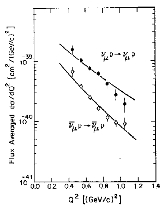
Figure 2.1: BNL E734 results on $\nu p\rightarrow\nu p$ and $\bar{\nu}p\rightarrow\bar{\nu}p$ [21]. The solid lines are fits to the data.

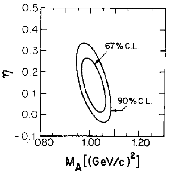
Figure 2.2: Results from a fit of the BNL E734 $\nu p\rightarrow\nu p$ and $\bar{\nu}p\rightarrow\bar{\nu}p$ scattering data [21] indicating the preferred values of $\eta$ ($=-\Delta s$) and $M_{A}$. In this fit, $M_{A}$ was constrained to the world-average value at the time $M_{A}=1.032\pm 0.036$ GeV.

This experiment also simultaneously measured the neutrino and antineutrino neutral current to charged current ratios:

$$R_{\nu}=\frac{\sigma(\nu p\rightarrow\nu p)}{\sigma(\nu n\rightarrow\mu^{-}p)}=0.153\pm 0.007\pm 0.017$$ (2.1)

and

$$R_{\bar{\nu}}=\frac{\sigma(\bar{\nu}p\rightarrow\bar{\nu}p)}{\sigma(\bar{\nu}p\rightarrow\mu^{+}n)},=0.218\pm 0.012\pm 0.023~{},$$ (2.2)

calculated over the interval $0.5<Q^{2}<1.0\,(\rm{GeV}/c)^{2}$. The dominant error in these ratios was an 11% systematic.

Reanalysis of BNL E734

The non-zero value for $\Delta s$ as obtained by BNL E734 was later reexamined [22]. This reanalysis more carefully considered the effects of strange contributions to the vector form factors and the $Q^{2}$ evolution of the axial form factor in the differential cross sections for $\nu p$ and $\bar{\nu}p$ elastic scattering. A value of $\Delta s=-0.21\pm 0.10$ was extracted. An additional form factor uncertainty of $\pm 0.10$, determined from fits to the data with different assumptions about the vector form factors and evolution of the axial form factor (via the axial vector mass, $M_{A}$), should be assigned.

Another group has reexamined the BNL E734 result on the neutral current to charged current ratios, $R_{\nu}$ and $R_{\bar{\nu}}$ [23]. These ratios are sensitive to the axial form factor, and avoid the systematic uncertainty of the neutrino flux and nuclear model corrections. While these ratios hold the promise of a superior method to extract $\Delta s$, the experimental errors from BNL E734 were too large to provide a definitive answer, and the conclusions of this analysis were consistent with the previous reanalysis of the data [22].

Another reanalysis of these data has been recently performed [17]. This approach is interesting in that it uses the latest data from HAPPEX on the electric and magnetic strange form factors in an effort to reduce the systematic errore from these form factors on this meausurement. The results show the viability of this method of combining the PV electron and neutrino scattering into one analysis, but are limited by the large systematic errors on the BNL734 data sample.

Note that the BNL E734 data have been reanalyzed at least three times since being published in 1987; this points to growing appreciation of the fact that neutral current neutrino scattering is an excellent probe of $\Delta s$. Unfortunately, though, the precision of the BNL E734 data limits the conclusions that can be drawn from it.

How FINeSSE Will Improve These Measurements

The neutrino neutral current to charged current ratio as measured by BNL E734 (Eq. 2.1) is reported with a statistical error of 5% and a systematic error of 11%. This ratio was made by integrating over the $Q^{2}$ interval $0.5<Q^{2}<1.0$ GeV².

FINeSSE will improve upon this measurement in several ways:

• The neutrino neutral current to charged current ratio measurement will be made as a function of $Q^{2}$ in the interval $0.2<Q^{2}<1.0$ GeV². FINeSSE’s measurement will be made at a lower-$Q^{2}$ value, where form factors are more easily interpreted. In addition, the shape of the ratio as a function of $Q^{2}$ holds additional information about the evolution of the form factors.

• With the proposed FINeSSE detector and run plan, the statistical errors in the $0.2<Q^{2}<0.4$ GeV²-bin alone will amount to a relative error on the ratio of only 2%.

• Systematic errors have been estimated with detailed simulations of the detector to be 5%. Much of this reduction in systematic error is due to the greatly reduced background in FINeSSE. The background to the $\nu p\rightarrow\nu p$ reaction is estimated at 26% (and is likely to be further reduced) compared to 40% in BNL E734 [21].

In summary, FINeSSE will be able to make a measurement of the neutral-current to charged-current ratio with a 6% total error down to $0.2$ GeV². BNL E734 made a measurement with 12% total error down to only $0.5$ GeV². This will allow a significant improvement to the uncertainty on the extracted value of $\Delta s$ as described in Section 2.1.3 and Chapter 5.

2.1.2 Relevance to Searches for Dark Matter

Understanding of the spin contribution to the nucleon of the strange quarks is important for certain searches of dark matter [24]. In $R$-parity-conserving supersymmetric models, the lightest supersymmetric particle (LSP) is stable and therefore a dark-matter candidate; in certain scenarios, the relic LSP density is large enough to be of cosmological interest. Experimental searches for cosmic LSPs can be competitive with accelerator-based searches [25].

In the case where the LSP is the neutralino, cosmic LSP can be detected either directly, through elastic neutralino scattering in an appropriate target/detector, or indirectly. The indirect method involves detection of high-energy neutrinos from the center of the sun, where the heavy neutralinos accumulate and subsequently annihilate. If the neutralino mass is larger than the $W$ mass, annihilation into gauge bosons dominates and this gives rise to high-energy neutrinos that can be detected on earth. The expected rate for this process also depends on the elastic neutralino-nucleon scattering cross section.

The neutralino-nucleus elastic-scattering cross section contains a spin-dependent and a spin-independent part. The spin-dependent part is given by

$$\sigma=\frac{32}{\pi}G_{F}^{2}m_{r}^{2}\Lambda^{2}J(J+1),$$

where $G_{F}$ is the Fermi constant, $m_{r}$ the reduced neutralino mass, $J$ the nucleus spin, and

$$\Lambda\equiv\frac{1}{J}\left(a_{p}\left\langle S_{p}\right\rangle+a_{n}\left\langle S_{n}\right\rangle\right);$$

here $\left\langle S_{p(n)}\right\rangle$ is the average proton (neutron) spin in the nucleus and

$$a_{p(n)}=\sum_{i}\frac{\alpha_{i}}{\sqrt{2}G_{F}}\Delta q_{i}^{p(n)},$$

where the sum is over quark flavors and the coefficients $\alpha_{i}$ are functions of the composition of the neutralino in terms of the supersymmetric partners of the gauge bosons. The factors $\Delta q_{i}^{p}$ and $\Delta q_{i}^{n}$ are the quark contributions to the proton or neutron spin.

It is established [18, 6] that $\Delta u$ and $\Delta d$ have opposite signs. From the above, it should be clear that knowledge of $\Delta s$ not only is important for the interpretation of any limits from such dark matter searches, but it could also influence the choice of detector material for direct searches [26], making nuclei with either proton- or neutron-spin excess optimal, depending on its value and sign.

2.1.3 A Measurement of $\Delta s$ via Neutral-Current Neutrino Scattering

In neutral current elastic (NC) neutrino-nucleon scattering ($\nu N\rightarrow\nu N$), any isoscalar contribution (such as strange quarks) to the nucleon spin will contribute to the cross section. This is in contrast to the charged current quasi-elastic (CCQE) scattering process ($\nu n\rightarrow\mu^{-}p$) where only isovector contributions are possible.

FINeSSE will use this feature of neutrino scattering to measure any contribution of strange quarks to the spin of the nucleon. The fact that NC neutrino scattering is sensitive to strange quark (isoscalar) spin in the proton, and CCQE neutrino scattering is not, will be exploited by measuring a ratio of these two processes; this will eliminate a number of experimental and theoretical errors.

The Neutral Weak Axial Current of the Nucleon

The axial part of the weak neutral current may be written [22, 27],

$$\left\langle N\left|A_{\mu}^{Z}\right|N\right\rangle = -\left[\frac{G_{F}}{\sqrt{2}}\right]^{\frac{1}{2}}\left\langle N\left|\frac{\bar{u}\gamma_{\mu}\gamma_{5}u-\bar{d}\gamma_{\mu}\gamma_{5}d-\bar{s}\gamma_{\mu}\gamma_{5}s}{2}\right|N\right\rangle$$ (2.3)

$$= -\left[\frac{G_{F}}{\sqrt{2}}\right]^{\frac{1}{2}}\left\langle N\left|-\frac{G_{A}(Q^{2})}{2}\gamma_{\mu}\gamma_{5}\tau_{z}+\frac{G_{A}^{s}(Q^{2})}{2}\gamma_{\mu}\gamma_{5}\right|N\right\rangle,$$ (2.4)

where $G_{A}$ is the axial form factor and $\tau_{z}=\pm 1$ for protons (+) or neutrons (-). The strange axial-vector form factor, $G_{A}^{s}$, is identified with the $\bar{s}\gamma_{\mu}\gamma_{5}s$ term which is $\Delta s$, the spin carried by the strange quarks. So, the non-strange ($u$ and $d$) quark axial current is accounted for in $G_{A}$, known at $Q^{2}=0$ from neutron beta decay to be $G_{A}(Q^{2}=0)=1.2673\pm 0.0035$ [28]. The (unknown) strange quark axial current is subsumed in $G_{A}^{s}$. A similar decomposition may be obtained for the vector part of the neutral weak current [22, 27] in terms of the two non-strange vector form factors, $F_{1}$ and $F_{2}$, and the corresponding strange quarks parts, $F_{1}^{s}$ and $F_{2}^{s}$.

As shown above, the strange axial form factor, $G_{A}^{s}$, in the limit of zero momentum transfer ($Q^{2}=0$), is identified with the strange quark contribution to the nucleon spin, $\Delta s$. It is worth mentioning that the arguments leading to the connection between $G_{A}^{s}$ at low momentum transfer and the strange spin content, $\Delta s$, that can be extracted from DIS data in the scaling limit, are essentially the same as those that were used to derive the Bjorken sum rule, which connects spin-dependent DIS structure functions to the coupling constants in neutron decay and is considered one of the most fundamental predictions of QCD. They are both based on the operator product expansion, which expresses the moments of structure functions in terms of matrix elements of local operators and perturbatively calculable Wilson coefficients.

Neutrino Cross Sections and Form Factors

The differential cross section, $d\sigma/dQ^{2}$, for NC and CCQE scattering of neutrinos and antineutrinos from nucleons can be written as a function of the nucleon form factors $F_{1}$ and $F_{2}$ (both vector) and $G_{1}$ (axial vector) [29, 27]:

$$\frac{d\sigma}{dQ^{2}}=\frac{G_{F}^{2}}{2\pi}\frac{Q^{2}}{E_{\nu}^{2}}(A\pm BW+CW^{2})$$ (2.5)

with kinematic factor, $W=4E_{\nu}/m_{p}-Q^{2}/m_{p}^{2}$. The + (-) sign is for neutrino (antineutrino) scattering. $Q^{2}$ is the squared-four-momentum transfer. The $A$, $B$, and $C$, contain the form factors:

$$A = \frac{1}{4}[G_{1}^{2}(1+\tau)-(F_{1}^{2}-\tau F_{2}^{2})(1-\tau)+4\tau F_{1}F_{2}],$$ (2.6)

$$B = -\frac{1}{4}G_{1}(F_{1}+F_{2}),$$ (2.7)

$$C = \frac{1}{16}\frac{m_{p}^{2}}{Q^{2}}(G_{1}^{2}+F_{1}^{2}+\tau F_{2}^{2}).$$ (2.8)

Up to this point, this formalism is valid for both NC and CCQE neutrino- (and antineutrino-) nucleon scattering. The difference between the NC and CCQE processes is accounted for with different form factors ($F_{1}$, $F_{2}$, and $G_{1}$) in each case.

For NC neutrino scattering the axial-vector from factor (as described in Section 2.1.3) may be written in terms of the known axial form factor plus an unknown strange form factor:

$$G_{1}=\left[-\frac{G_{A}}{2}\tau_{z}+\frac{G_{A}^{s}}{2}\right].$$ (2.9)

The vector form factors $F_{1,2}$ may also be written in terms of known form factors plus a strange quark contribution,

$$F_{1,2}=\left[\left[\frac{1}{2}-\sin^{2}\theta_{W}\right]\left[F_{1,2}^{p}-F_{1,2}^{n}\right]\tau_{z}-\sin^{2}\theta_{W}\left[F_{1,2}^{p}+F_{1,2}^{n}\right]-\frac{1}{2}F_{1,2}^{s}\right]~{},$$ (2.10)

where $F_{1}^{p(n)}$ is the Dirac form factor of the proton (neutron) and $F_{2}^{p(n)}$ is the Pauli form factor. The CVC hypothesis allows us to write the same form factors in these equations as those measured in electron scattering. Therefore, the only unknown quantities in these equations are the strange vector form factors $F_{1,2}^{s}$.

The differential cross section for neutrino scattering at low $Q^{2}$(Eq. 2.5) is dominated by the axial form factor, $G_{1}$. This can be seen be examining Equations 2.5 and 2.6. In fact, at low-$Q^{2}$, $d\sigma/dQ^{2}\propto G_{1}^{2}$. This is a crucial point, and it is what makes NC neutrino scattering the best place to look for the effects of strange-quarks in the nucleon spin. It also makes the results less sensitive to the strange vector form factors, $F_{1,2}^{s}$.

$Q^{2}$ Dependence of the Form Factors

All of the form factors are, most generally, functions of $Q^{2}$. The values of the non-strange form factors at $Q^{2}=0$ are known from the static properties of the nucleon (e.g. charge, magnetic moment, and neutron decay constant). How the form factors change with increasing $Q^{2}$ is less well known and must be addressed. The form factors are commonly parameterized with a dipole form, where the dipole mass set by various measurements. The evolution of $F_{1,2}^{p(n)}$ is known via numerous experiments on electron scattering; the vector dipole mass, $M_{V}$ is 0.843 GeV/c². The $Q^{2}$ dependence of the axial form factor, $G_{A}$, is measured via CCQE neutrino scattering; the world average data yield an axial mass $M_{A}=1.026\pm 0.021$ [28].

Both the strange form factors, $F_{1,2}^{s}$ and $G_{A}^{s}$ and their $Q^{2}$ evolution are unknown. It is most common to assume the same $Q^{2}$ dependence as for the non-strange form factors, using $M_{V}$ for $F_{1,2}^{s}$ and $M_{A}$ for $G_{A}^{s}$. The uncertainty on the $Q^{2}$ evolution introduces some uncertainty in the extraction of $G_{A}^{s}$ from a measurement. A measurement at $Q^{2}\approx 0.2$ GeV², however, would keep this contribution to the uncertainty at a low level, as the value of the form factor differs by only 20% from $Q^{2}=0$ to $Q^{2}=0.2$ GeV².

Nuclear Physics Corrections

The expression for the cross section (Eq. 2.5) is for scattering from free nucleons. Since FINeSSE will have a target that consists, in large part, of nucleons bound in carbon, consideration will need to be given of the effects of this binding [30, 31]. The corrections can be rather large when considering the absolute event rate, and can depend greatly on the model employed, because the amount and quality of available neutrino data to constrain such models, is lacking. In principle, the nuclear models can be constrained with the high-quality electron data available; this, however, is a work in progress.

These effects become less of a concern when ratios of cross sections are considered [32, 33, 34, 35]. The initial and final states of the hadrons involved are quite similar in both NC and CCQE neutrino scattering; as a result, the corrections employed for either channel should be similar as well. FINeSSE will utilize this fact with a measurement of $\Delta s$ as explained in the following sections.

The Neutral Current to Charged Current Ratio

The NC neutrino scattering cross section depends strongly on $G_{1}$ and therefore on $G_{A}^{s}$, the quantity of interest. An absolute measurement of the cross section, however, is an experimental challenge; the level of precision achievable for this measurement would not yield the desired precision for $G_{A}^{s}$. An absolute prediction is also a challenge from a phenomenological standpoint, as uncertainties in form factors and nuclear corrections can be large.

It is possible to extract $G_{A}^{s}$ to the desired precision by measuring the ratio of NC to CCQE event rates. A measurement of the ratio of NC to CCQE neutrino scattering event rates may be measured with greater precision, since many systematic uncertainties cancel in the ratio such as the neutrino flux and correlated reconstruction efficiencies. Theoretical uncertainties are also reduced in this quantity as many of these uncertainties are correlated between NC and CCQE scattering. FINeSSE will use this method to measure $G_{A}^{s}$.

First, consider the ratio of NC neutrino-proton to NC neutrino-neutron scattering,

$$R(p/n)=\frac{\sigma(\nu p\rightarrow\nu p)}{\sigma(\nu n\rightarrow\nu n)}.$$ (2.11)

This ratio is very sensitive to $G_{A}^{s}$ [27]. The NC neutrino nucleon scattering cross section is proportional to $G_{1}^{2}$ as explained above. A non-zero value for $G_{A}^{s}$ will pull the denominator of this ratio one way, and the numerator the other, due to the $\tau_{z}$ factor in Equation 2.9.

$R(p/n)$, however, is likely to be very difficult to measure accurately in a neutrino scattering experiment, because of the intrinsic difficulties and uncertainties involved with neutron detection. For this reason FINeSSE will focus on a measurement of the ratio of the NC neutrino-proton scattering ($\nu p\rightarrow\nu p$) to CCQE neutrino scattering ($\nu n\rightarrow\mu^{-}p$). This ratio,

$$R(NC/CC)=\frac{\sigma(\nu p\rightarrow\nu p)}{\sigma(\nu n\rightarrow\mu^{-}p)},$$ (2.12)

can be more accurately measured and is still quite sensitive to $G_{A}^{s}$ (albeit less so than $R(p/n)$). The numerator depends upon $G_{A}^{s}$ as explained in the formalism introduced above. The denominator does not as the $\nu n\rightarrow\mu^{-}p$ process is sensitive only to isovector quark currents and not to isoscalar currents (such as that from strange quarks).

The $\nu p\rightarrow\nu p$ and $\nu n\rightarrow\mu^{-}p$ differential cross sections (weighted by the calculated FINeSSE flux) as calculated with Equation 2.5 are plotted in Figure 2.3 for $G_{A}^{s}=-0.1,0.0,+0.1$; this shows that the cross section for $\nu p\rightarrow\nu p$ depends strongly upon $G_{A}^{s}$. The cross section for $\nu n\rightarrow\mu^{-}p$ is independent of $G_{A}^{s}$, so the ratio of flux-weighted cross sections (and therefore the event rates) of these two processes depends upon $G_{A}^{s}$.

Figure 2.3: Flux-weighted differential cross section as a function of $Q^{2}$ for $\nu p\rightarrow\nu p$ (a) and $\nu n\rightarrow\mu^{-}p$ (b) scattering together with the cross section ratio of the these two processes (c). These quantities are shown for $G_{A}^{s}=0.$ (solid), $=-0.1$ (dashed), and $=+0.1$ (dotted). The $\nu n\rightarrow\mu^{-}p$ process does not depend upon $G_{A}^{s}$.

This dependence is also shown in Figure 2.4 as a function of $G_{A}^{s}$ for three different $Q^{2}$ bins. In the $Q^{2}=0.25$ GeV² bin, the sensitivity of the NC/CC ratio on $G_{A}^{s}$ is approximately 1.2. The relative uncertainty in the NC/CC ratio, $\Delta R/R$ is related to the absolute uncertainty on $G_{A}^{s}$, $\sigma(G_{A}^{s})$ by

$$\sigma(G_{A}^{s})=\frac{1.0}{1.2}\frac{\Delta R}{R}.$$ (2.13)

Figure 2.4: Ratio of flux-weighted cross sections of the $\nu p\rightarrow\nu p$ and $\nu n\rightarrow\mu^{-}p$ processes as a function of the axial form factor $G_{A}^{s}$ at $Q^{2}=0.25$ (solid), 0.45 (dashed), and 0.65 (dotted) GeV².

Considering this and recalling that $G_{A}^{s}(Q^{2}=0)=\Delta s$ yields the conclusion that a 5% relative measurement of the NC/CC ratio at $Q^{2}\approx 0.25$ GeV² would enable an extraction of $\Delta s$ with an error of 0.04. This error is comparable to that quoted in the latest extractions of $\Delta s$ from charged lepton DIS [20].

2.1.4 FINeSSE Sensitivity to $\Delta s$

NC, CCQE, and background events in the proposed detector have been simulated in a detailed manner; a reconstruction procedure has been performed, to calculate an estimated sensitivity. All conceivable effects were considered; systematic errors were estimated. The experimental errors considered were those due to statistics and to various systematics. The statistical errors were calculated based on a 9 ton (fiducial) detector running for two years ($6\times 10^{20}$ protons-on-target). The systematic uncertainties considered include those due to free-to-bound $\nu p\rightarrow\nu p$ scattering rate, reconstruction efficiencies, background estimation, and $Q^{2}$ reconstruction. In addition, theoretical uncertainties from nuclear model dependence and from form factor estimation were considered. The details of this procedure are described in Chapter 5.

A fit to the simulated data in the $Q^{2}$ region where the detector has reasonable acceptance yields an experimental uncertainty in $\Delta s$ of $\pm 0.039$; the combined uncertainty from the axial mass, $M_{A}$, and $F_{2}^{s}$ form factor is $\pm 0.025$.

Based on these results, it has been determined that FINeSSE, with a design and plan described in the Chapters below, can make an accurate measurement of $\Delta s$ at down to $Q^{2}\approx 0.2$ GeV². This will enable FINeSSE to answer an important and unresolved question about the structure of the proton.

2.2 $\nu_{\mu}$ Disappearance

The FINeSSE detector can be used in conjunction with the MiniBooNE detector to substantially improve our understanding of neutrino oscillations at high $\Delta m^{2}$ by looking for a neutrino energy-dependent deficit of $\nu_{\mu}$ event rates compared to a no-oscillation hypothesis. This search is motivated by astrophysical models for the production of heavy elements in supernovae. If MiniBooNE observes a signal, a combined FINeSSE and MiniBooNE (“FINeSSE+MiniBooNE”) run represents the next step in determining the underlying physics model of the oscillation. These two motivations are not directly connected: if MiniBooNE does not see a signal, the astrophysical case still makes this study compelling.

In this section, we first provide a brief overview of the formalism for neutrino oscillations. Second, we introduce the LSND signal, along with theoretical interpretations involving sterile neutrinos. Third, we describe the astrophysical motivations for the disappearance search. Lastly, we describe the capability of a FINeSSE+MiniBooNE joint analysis of $\nu_{\mu}$ disappearance.

2.2.1 Neutrino Oscillation Formalism

“Neutrino oscillations” occur when a pure flavor (weak) eigenstate born through a weak decay changes into another flavor as the state propagates in space. This can occur if two conditions are met. First, the weak eigenstates can be written as mixtures of the mass eigenstates, for example:

$$\begin{array}[]{l}\nu_{e}=\cos\theta\;\nu_{1}+\sin\theta\;\nu_{2}\\ \nu_{\mu}=-\sin\theta\;\nu_{1}+\cos\theta\;\nu_{2}\end{array}$$

where $\theta$ is the “mixing angle.” The second condition is that each of the mass eigenstate components propagate with a different frequency, which can occur only if the masses are different. We define the squared mass difference as $\Delta m^{2}=\left|m_{2}^{2}-m_{1}^{2}\right|>0$. In a two-component model, the oscillation probability for $\nu_{\mu}\rightarrow\nu_{e}$ oscillations is then given by:

$${\rm Prob}\left(\nu_{\mu}\rightarrow\nu_{e}\right)=\sin^{2}2\theta\;\sin^{2}\left(\frac{1.27\;\Delta m^{2}\left({\rm eV}^{2}\right)\,L\left({\rm km}\right)}{E\left({\rm GeV}\right)}\right)~{},$$ (2.14)

where $L$ is the distance from the source, and $E$ is the neutrino energy.

Most neutrino oscillation analyses consider only two-generation mixing scenarios, but the more general case includes oscillations between all neutrino species. For the case of the three Standard Model species, this can be expressed as:

$$\left(\begin{array}[]{l}\nu_{e}\\ \nu_{\mu}\\ \nu_{\tau}\end{array}\right)=\left(\begin{array}[]{lll}U_{e1}&U_{e2}&U_{e3}\\ U_{\mu 1}&U_{\mu 2}&U_{\mu 3}\\ U_{\tau 1}&U_{\tau 2}&U_{\tau 3}\end{array}\right)\left(\begin{array}[]{l}\nu_{1}\\ \nu_{2}\\ \nu_{3}\end{array}\right).$$

The oscillation probability is then:

$$P(\nu_{\alpha}\rightarrow\nu_{\beta}) = |\mbox{Amp}[\nu_{\alpha}\rightarrow\nu_{\beta}]|^{2}=\delta_{\alpha\beta}$$ (2.15)

$$\mbox{}-4\sum_{i>j}\Re\,(U^{*}_{\alpha i}U_{\beta i}U_{\alpha j}U^{*}_{\beta j})\sin^{2}[\Delta m^{2}_{ij}(L/4E)]$$

$$\mbox{}+2\sum_{i>j}\Im\,(U^{*}_{\alpha i}U_{\beta i}U_{\alpha j}U^{*}_{\beta j})\sin[\Delta m^{2}_{ij}(L/2E)]~{},$$

where $\Delta m_{i\,j}^{2}=\left|m_{i}^{2}-m_{j}^{2}\right|$. Note that there are three different $\Delta m^{2}$ (although only two are independent), and three different mixing angles. This method can be generalized to include more neutrino species in Beyond-the-Standard Model Theories.

Although in general there will be mixing among all flavors of neutrinos, two-generation mixing is often assumed for simplicity. If the mass scales are quite different (e.g., $m_{3}>>m_{2}>>m_{1}$), then the oscillation phenomena tend to decouple and the two-generation mixing model is a good approximation in limited regions. In this case, each transition can be described by a two-generation mixing equation. However, it is possible that experimental results interpreted within the two-generation mixing formalism may indicate very different $\Delta m^{2}$ scales with quite different apparent strengths for the same oscillation. This is because, as is evident from equation 2.15, multiple terms involving different mixing strengths and $\Delta m^{2}$ values contribute to the transition probability for $\nu_{\alpha}\rightarrow\nu_{\beta}$.

From equation 2.14, one can see that the oscillation wavelength will depend upon $L$, $E$, and $\Delta m^{2}$. For short baseline experiments, sensitivity to oscillations is in a range of $>0.1$eV², which will term the “high $\Delta m^{2}$ region. The oscillation amplitude will depend upon $\sin^{2}2\theta$.

2.2.2 Experimental Results: The LSND Signal

One of the most exciting questions in high energy physics, at present, is whether the “LSND signal” is due to neutrino oscillations. If the signal is confirmed in the MiniBooNE experiment, then this is an indication for new physics beyond the Standard Model. Fermilab will want to be poised to pursue this result. A FINeSSE+MiniBooNE run will be the first step.

The LSND experiment has observed a 4$\sigma$ excess which can be interpreted as oscillations between muon and electron neutrinos [36]. The beam was produced at LANSCE at LANL, with 800 MeV protons interacting with a water target, a close-packed high-Z target, and a water-cooled copper beam dump. The highest statistics came from $\bar{\nu}_{\mu}$ neutrinos produced by decay at rest (DAR) of muons, with $20<E<50$ MeV. However, the lower statistics decay in flight (DIF) $\nu_{\mu}$’s were also analyzed. The liquid scintillator detector was located 30 m from the beam dump. Hence the $L/E$ of the experiment was $\sim 1$ m/MeV. As a result, if the excess is interpreted as oscillations, the allowed region is located at high $\Delta m^{2}$.

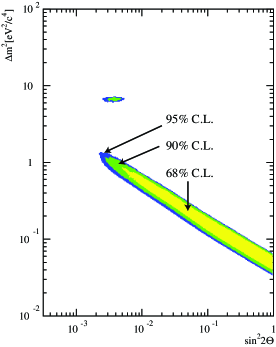
Figure 2.5: LSND and Karmen joint analysis allowed region.

LSND is the only short-baseline experiment to have observed evidence for oscillations. Other short-baseline experiments have searched and seen no signal. Those most relevant to this proposal are Karmen [37] and Bugey [38]. Karmen, which ran at the ISIS facility at Rutherford Labs, was similar in concept to LSND, using a DAR beam; but the detector was smaller, and the beam of lower intensity. Most importantly, it had an L of 17 m; in this way, it can be thought of as a “near detector” for LSND. Playing the null signal in Karmen against the observed excess in LSND results in the allowed regions shown in Figure 2.5 [39]. The Bugey reactor experiment rules out $\sin^{2}2\theta>0.04$ at 90% C.L. in a search for $\bar{\nu}_{e}$ disappearance using a reactor. Assuming that oscillations respect time reversal, and that only the three standard model active species are involved, Bugey’s result can be taken as an excluded region for LSND.

The MiniBooNE experiment is a designed to decisively address the LSND signal. This experiment will complete its Phase I (neutrino) run in mid-2005 and is expected to request further (Phase II) running for the period thereafter. By the time FINeSSE is on-line, the LSND signal will be tested in both $\nu$ and $\overline{\nu}$ modes.

If MiniBooNE confirms LSND, and all other oscillation results remain as they presently stand, then this necessarily implies new physics. The oscillation signals from solar neutrinos, atmospheric neutrinos, and LSND cannot be simultaneously fit with the three Standard Model neutrinos. A favored method for expanding the theory to allow LSND is to invoke sterile neutrinos ($\nu_{s}$). These are neutrinos which do not interact via the W or Z, but can couple to the Standard Model “active” neutrinos through oscillations. The most minimal extension is to introduce a single light sterile neutrino. This extra neutrino is not ruled out by cosmology [40]. Light sterile neutrinos can appear in supersymmetry, extra dimensions and GUTs [41]. These can all accommodate more than one light sterile neutrino, but we will confine our discussion to one for simplicity.

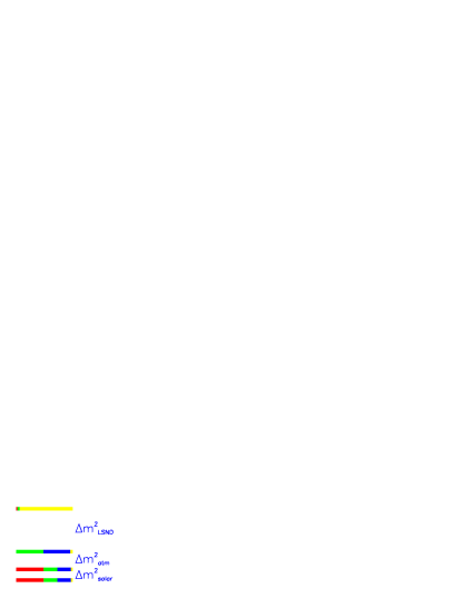
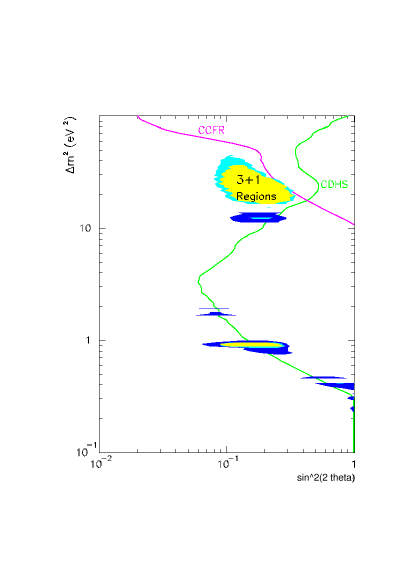
Figure 2.6: Left: an example of a 3+1 mass spectrum. Right: allowed region for $\nu_{\mu}\rightarrow\nu_{s}$ in 3+1 models. The exclusion regions for CDHS and CCFR are also shown.

Figure 2.6(left) shows a cartoon of how the squared masses and mixings might be arranged if a single sterile neutrino is introduced into the theory. The vertical axis is logarithmic and arbitrary. The bars indicate the flavor content of each mass state. The LSND signal is explained by the largest squared mass splitting, with the transition $\nu_{\mu}\rightarrow\nu_{e}$. Because there is a triplet of neutrinos with nearly the same mass, and one large splitting, this is called a “3+1” model. Note that the transitions $\nu_{\mu}\rightarrow\nu_{s}$ and $\nu_{e}\rightarrow\nu_{s}$ must also be allowed for the same $\Delta m^{2}$. The allowed regions for 3+1 for fits which include LSND, Karmen, Bugey, and two $\nu_{\mu}$ disappearance experiments (CDHS and CCFR84) are shown in Figure 2.6(right) [42]. These allowed regions can be addressed by FINeSSE+MiniBooNE as discussed below.

2.2.3 Astrophysical Motivation for High $\Delta m^{2}$ Disappearance Searches

The existence of at least one sterile neutrino in the high $\sim 1$ eV mass range has interesting consequences for the heavy element abundance in the universe. In fact, oscillations were predicted on the basis of this abundance before the LSND signal was presented [3]. The allowed range extends beyond the region constrained by the LSND signal. Hence, whether or not MiniBooNE confirms LSND, searches for active-to-sterile oscillations at high $\Delta m^{2}$ remain motivated by this astrophysical question.

Active-to-sterile neutrino oscillations in the late time post-core-bounce period of a supernova will affect the $r$-process, or rapid neutron capture process. This presents a mechanism for producing substantially more heavy elements ($A>100$), solving the long-standing problem of the high abundance of uranium in the universe. The FINeSSE+MiniBooNE search addresses allowed parameters for this solution.

A favored mechanism for producing heavy elements is through the $r$-process in the neutrino-heated ejecta of a Type II or Type I/c supernova. In this model, during the period of the neutrino-driven wind, which lasts for $\sim 10$s, “seed” elements with $A$ between 50 and 100 capture neutrons to produce the elements with $A>100$. The problem is that in most models the neutron-to-seed ratio, $R$, is too low for production of the heaviest elements [43]. In fact, detailed simulation show that a phenomenon called the $\alpha$-effect, in which neutrons are frozen into alpha particles that do not recombine to form heavier elements in the requisite time period, renders the neutron-to-seed ratio downright “anemic” [44].

Various solutions have been proposed. One option is to resort to the competing theory of neutron star mergers. The problem with this scenario is that mergers are too rare to produce the observed abundance of heavy elements [45]. Another alternative is to introduce physics which adjusts the neutron-to-seed ratio. This can be done by modifying the expansion rate, the entropy per baryon or the $n/p$ ratio – all of which will affect the neutron-to-seed ratio. Adjusting any of these three requires invoking new physics in the model. We explore the last alternative here: introducing $\nu_{e}\rightarrow\nu_{sterile}$ oscillations, which, when combined with matter effects, enhance the production of neutrons over protons.

The idea [46, 44] is that production of neutron-rich elements requires a neutron-rich environment. To the level that the processes $\nu_{e}+n\rightarrow p+e^{-}$ and $\bar{\nu}_{e}+p\rightarrow n+e^{+}$ are in balance during the neutrino-driven wind, there is no net excess of neutrons. In its simplest form, neutrino oscillations between an electron and sterile flavor would not upset the balance because $\nu_{e}$ and $\bar{\nu}_{e}$ will oscillate at the same rate. However, when one introduces matter (or MSW [47]) effects, neutrino and anti-neutrino oscillations are modified with opposite sign in an electron-rich environment. Oscillations of $\nu_{e}$ to sterile neutrinos are enhanced, while $\bar{\nu}_{e}$ are depressed. This can produce a substantial neutron excess by removing the offending $\nu_{e}$’s. The $\alpha$-process removes some neutrons, but stalls once the protons are devoured, leaving sufficient neutrons to produce the high-$A$ elements.

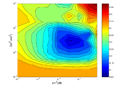
Figure 2.7: Allowed oscillation parameters for the oscillation-enhanced $r$-process.

In this model, the neutron-to-proton ratio (usually characterized as the function $Y_{e}=1/(1+n/p))$), depends upon the choice of $\Delta m^{2}$ and $\sin^{2}2\theta$. The condition for a successful r-process is $Y_{e}<1/2$. The smaller the value of $Y_{e}$, the larger the high-$A$ abundance. Figure 2.7 shows $Y_{e}$ as a function of the $\nu_{e}\rightarrow\nu_{s}$ oscillation parameters. This shows that there are a wide range of “robust” solutions [44].

One can connect the allowed space for $\nu_{\mu}\rightarrow\nu_{s}$ and $\nu_{\mu}\rightarrow\nu_{e}$ to the allowed region for $\nu_{e}\rightarrow\nu_{s}$ within 3+1 and 3+2 models. If MiniBooNE sees a signal, this will be a great victory for the oscillation-enhanced r-process model. In the case where MiniBooNE does not see a signal, there remains a large parameter space open to this model. At present, $\nu_{\mu}$ disappearance in FINeSSE+MiniBooNE represents the only way to access that parameter space.

2.2.4 FINeSSE+MiniBooNE Capability for $\nu_{\mu}$ Disappearance

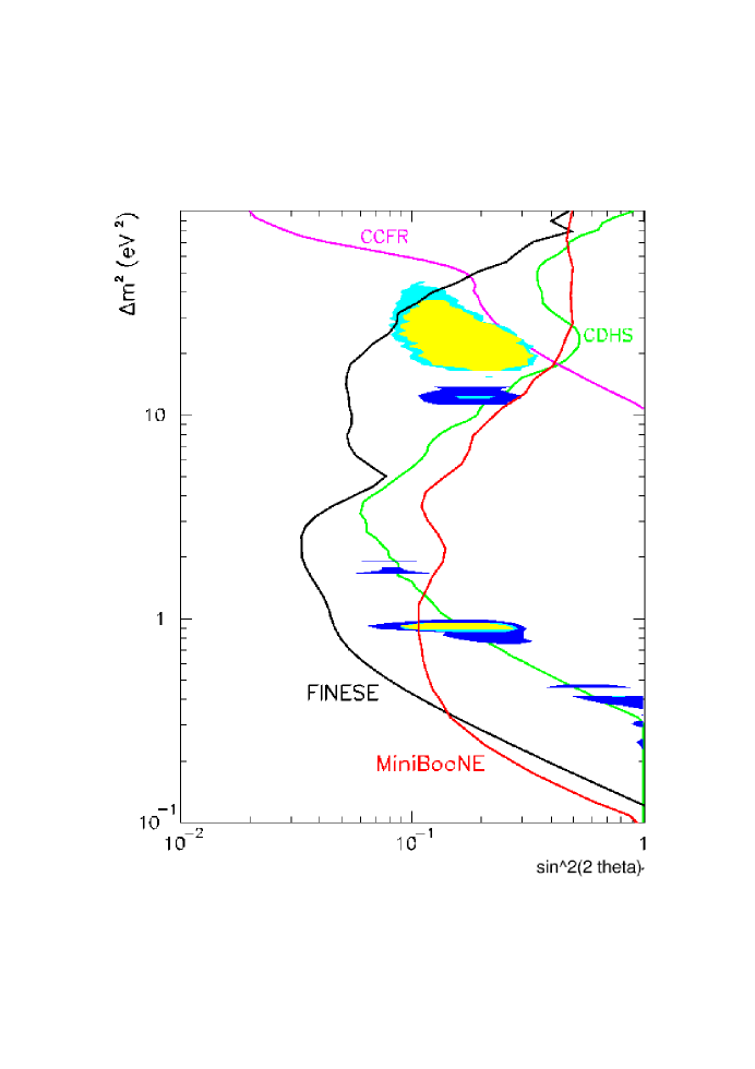
Figure 2.8: The parameter space covered by FINeSSE+MiniBooNE for $\nu_{\mu}$ disappearance (labeled “FINESE”). Also shown: allowed regions in 3+1 models given the LSND signal (solid), existing exclusion regions from CDHS and CCFR, and the expected exclusion region for MiniBooNE.

The FINeSSE detector can be combined with MiniBooNE to explore allowed regions for oscillations to sterile neutrinos via $\nu_{\mu}$ disappearance. In this analysis, FINeSSE serves as a near detector to accurately measure the flux, and MiniBooNE serves as the far detector where a deficit may be observed. This is a unique capability – there are no other short baseline $\nu_{\mu}$ disappearance experiments in the world. If MiniBooNE observes a signal, FINeSSE+MiniBooNE will be a crucial next-step toward understanding the result. If MiniBooNE does not observe a signal, this region is still interesting because of its relevance to astrophysics.

Figure 2.8 shows the FINeSSE+MiniBooNE expectation for the default design, with $6\times 10^{20}$ protons on target, in neutrino mode. Also shown are the 3+1 allowed regions for fits to LSND, atmospheric, and solar (as described above); and the expectation for MiniBooNE prior to FINeSSE running. MiniBooNE will be able to address the lower 3+1 allowed regions. The largest 3+1 allowed region, however, can only be addressed by the FINeSSE+MiniBooNE combination. This combination of FINeSSE and MiniBooNE is therefore very powerful; it alone is able to address the full 3+1 picture.

The“standard” configuration for FINeSSE and MiniBooNE simultaneous running places the FINeSSE detector at 100 m from the primary beryllium target, with the 25 m absorber installed in the beamline. The angular acceptance from the target to FINeSSE is 25 mrad, and to MiniBooNE is 10 mrad. In this analysis, we accept only neutrinos which traverse both detectors, meaning that we use only the inner 1 m radius (10 mrad acceptance from target) of FINeSSE. Event rates are for a 9 ton fiducial volume and $6\times 10^{20}$ protons in neutrino mode.

In Chapter 5, we provide details on how the sensitivity shown in Figure 2.8 was obtained. We explain why the standard configuration is best for the analysis. We also describe the method for determining the sensitivity, which compares the energy distribution of events in the near and far detector. This method accounts for both statistical and systematic errors.

2.3 FINeSSE on the Booster Neutrino Beamline

The Booster neutrino beamline is the only existing beamline at Fermilab or around the world where this physics can be accomplished. The FINeSSE $\Delta s$ measurement requires a clean, low energy neutrino spectrum, as is produced by the Booster neutrino production target. The oscillation physics goals of FINeSSE require the energies and baselines available to experiments on the Booster neutrino beamline. These requirements make it impossible to perform this measurement at Fermilab’s other existing neutrino beamline, NuMI.

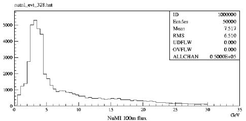
Figure 2.9: The flux spectrum of the Booster neutrino beam and the NuMI neutrino beam at their near detector locations.

Figure 2.9 shows the NuMI beam flux at the MINOS near detector location, 290 m from the NuMI decay pipe. The Booster neutrino spectrum at 75 m from the end of the Booster neutrino beamline decay pipe with the 25 m absorber in position (100 m from the production target), is shown in Figure 3.2. As indicated, the average energy of neutrinos from the Booster is 700 MeV, with virtually no neutrinos beyond 3 GeV. This neutrino energy distribution is excellent for making the $\Delta s$ measurement. It is an energy large enough to be beyond the region where low-energy nuclear corrections are significant, yet not so large where pion production and DIS scattering backgrounds are high. The NuMI flux, however, has an average energy above 7 GeV and a tail that extends past 30 GeV. This energy distribution creates large pion and DIS scattering rates that increase the background to NC neutrino elastic scattering considerably.

In addition, this flux of neutrinos around the MINOS near detector enclosure will create a large flux of low-energy neutrons from neutrino interactions in the earth. This background is much larger in the MINOS area when compared to that in FINeSSE. The results of simulation of this effect are shown in Figure 2.10. Note that in the lowest energy bin, the background is 14 times higher at the MINOS near detector location. For these reasons, the $\Delta s$ measurement can not be made in the NuMI beam.

Figure 2.10: Ratio of neutron background, from neutrino interactions in the surrounding earth, to NC-like detector events using the FINeSSE detector in the Booster neutrino beam (top) and the NuMI neutrino beam (bottom), shown as a function of energy energy deposited in the detector. This plot assumes 100% detection and reconstruction efficiency.

In order to explore the oscillation regions discussed in Section 2.2.4, a two detector comparison is required, and L/E for the far detector must be on the order of 1 m/MeV. This is not possible in the NuMI beamline for two reasons. First, there is no tunnel for a detector far enough upstream of the MINOS near detector (equivalent to the FINeSSE detector) to measure the beam before the neutrinos have oscillated. Second, the high average neutrino energy of the NuMI beam means that the baseline for the far detector for an oscillation experiment would have to be on the order of 800 m, a much longer distance than is available in the NuMI beamline. These two consideration lead to the conclusion that FINeSSE must run on the Booster neutrino beamline.

Chapter 3 The Neutrino Beam and Expected Event Rates

3.1 The Booster Neutrino Beam

The Booster neutrino beamline presently delivers beam to the MiniBooNE experiment; as the FINeSSE detector will be placed upstream of MiniBooNE, the one beamline will provide neutrinos to both experiments. The projections for protons on target (POT) in this section are based on a conservative interpretation of the Proton committee report [5].

3.1.1 Beam Intensity Requirements

During the fall 2003 shutdown, several improvements in the Booster were made. These upgrades are expected to provide routine peak operation with $5\times 10^{12}$ protons/batch and 5 Hz for the Booster neutrino beamline. The efficacy of these improvements will be understood prior to FINeSSE running, and there should also be sufficient time to implement additional improvements if the goals are not met by the end of 2004.

By the summer of 2003, the Booster was routinely delivering more than 5$\times 10^{12}$ protons/batch for Stacking for Run II, demonstrating that Booster can achieve the batch intensity required for FINeSSE. The issues are reducing and controlling losses at this intensity, and achieving the required repetition rate. The principal improvements during the Fall of 2003 were modifications to the doglegs to reduce losses, installation of two large aperture RF cavities to reduce losses at these two locations, the installation of collimators to control losses, and modifications to the RF and magnet subsystems to allow an increase of the equipment repetition rate to 7.5 Hz. Once these improvements are operational, it is expected that the above ground radiation will be the limit on Booster operation; however, this limit is well above what is needed during the FINeSSE era. In addition, in 2004, Fermilab and Columbia University are expected to develop a robot for measuring the losses in the Booster during beam operation, which will help to understand these losses in detail.

Although the Booster equipment may be able to achieve 7.5 Hz, the MiniBooNE horn imposes a limit of 5 Hz. If the Booster were to achieve 5$\times 10^{12}$ protons/batch at 5 Hz for an hour, the MiniBooNE target would receive 9$\times 10^{16}$ protons per hour. This is considered a nominal performance level, however, and it is not expected to persist for a week, (much less for an entire year).

To relate a nominal performance to the number of protons delivered per year, one can define an annual efficiency. The analysis used here follows the same steps given in the Proton committee report [5]. The annual efficiency must include factors to account for the number of weeks actually scheduled for beam operation in a year; the reliability of the Proton Source (Linac, Booster, and beam transfer lines) during those scheduled weeks; and the operational efficiency for actually achieving 5$\times 10^{12}$ protons/batch and 5 Hz. The number of weeks scheduled per year is determined by the Director’s Office and is taken to be in the range 42 to 44 weeks. The reliability of the Proton Source has been measured by MiniBooNE to be in the range 0.90 to 0.94. The operational efficiency is estimated to be 0.90 [48]. Combining these factors one obtains an annual efficiency of 0.66 to 0.72.

By the time FINeSSE would start to run, however, NuMI will also be taking beam. NuMI is expected to use five Booster batches per Main Injector cycle. NuMI is expected to share the same Main Injector cycle as Stacking for Run II, and Stacking is expected to take two Booster batches per Main Injector cycle. The Main Injector cycle time is expected to be about two seconds. With these assumptions, NuMI plus Stacking will require seven batches every two seconds, which is an average rate of 3.5 Hz. At the moment, some of the Booster equipment requires two “prepulses” with no beam, or 1 Hz. Thus, the bandwidth required by NuMI, Stacking, and the prepulses is 4.5 Hz. This leaves 3 Hz for delivering beam to the MiniBooNE target, assuming a total Booster bandwidth of 7.5 Hz. This is 60% of the maximum 5 Hz which the Booster neutrino beamline should be receiving in 2004. If prepulses can be eliminated, then this can be used to add 1 Hz to this beamline, but this proposal does not count on that.

Thus, one expects a nominal performance of the Booster neutrino beam for FINeSSE of 5$\times 10^{12}$ protons/batch and 3 Hz. Given the range for annual efficiency calculated above, one calculates the POT/year for FINeSSE as 5$\times 10^{12}\times$ 3 Hz x 3.15$\times 10^{7}$ sec/yr x (0.66 to 0.72) = (3.12 to 3.40) $\times 10^{20}$ POT/yr.

This proposal assumes delivery of 3.0$\times 10^{20}$ POT/yr, conservatively below the range quoted above.

3.1.2 Booster Neutrino Beam Production

The Neutrino Flux

The neutrino beam is produced by the 8 GeV Fermilab Booster which currently feeds the MiniBooNE experiment. Protons from the Booster strike a 71 cm beryllium target inserted in a magnetic focusing horn. Protons arrive at this target in 1.6 $\mu$s long Booster spills. The timing structure within each spill delivers 84 2 ns wide bunches of beam, each separated by 18 ns. Secondary short-lived hadrons (primarily pions) produced in the target are focussed by the horn and enter a decay region. In normal MiniBooNE operation, this decay region is 50 m long, at the end of which region is a beam absorber to stop hadrons and low energy muons. Located 25 m from the proton target is an intermediate absorber which can be lowered into the beam for use as a systematic check on the MiniBooNE $\nu_{e}$ background from $\mu$ decays. It is assumed that the 25 m absorber will be in place during the period when FINeSSE is operational to accommodate FINeSSE and MiniBooNE physics goals. Figure 3.1 provides a diagram of the two possible absorber positions.

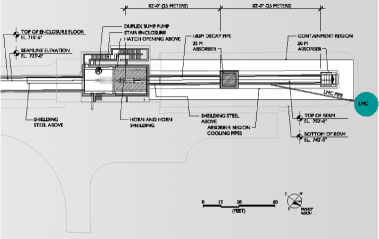
Figure 3.1: Schematic of the MiniBooNE target hall and decay region. The 25 m and 50 m absorber locations are indicated.

Figure 3.2: Expected $\nu_{\mu}$ flux at a 100 m detector site assuming a 25 m decay length.

The neutrino flux resulting from this design was simulated using the same tools currently being employed by the MiniBooNE collaboration [4]. The beam simulation utilizes GEANT 4 transport code [49], and the MiniBooNE JAM pion production model [50] which includes all beamline elements (horn, shielding, absorbers, etc.) and $\pi^{\pm}$, $K^{\pm}$, $K^{0}$ production from proton interactions on beryllium. To better reproduce the energy distribution of neutrino events observed in the MiniBooNE detector, pion spectra were input from a Sanford-Wang-based global fit [50] to pion production data in the relevant energy range in a procedure similar to that adopted by K2K. Figure 3.2 shows the resultant muon neutrino flux expected from a 25 m decay length beam produced at the 100 m FINeSSE detector site. In this configuration, $9.55\times 10^{-9}$ muon neutrinos per POT per cm² are anticipated with a mean energy of $\sim 700$ MeV. The neutrino flux is roughly 20 times larger than that expected in a comparable volume at MiniBooNE. Note that the flux is diminished by about a factor of 1.8 in switching from a 50 m decay length to a shorter 25 m decay length. However, as will be demonstrated, the 25 m absorber location is ideal for optimizing FINeSSE’s oscillation sensitivity.

Figure 3.3: Predicted flux contributions at a 100 m detector site assuming a 25 m decay length. Muon neutrinos comprise $93.5\%$ of the expected neutrino flux.

Figure 3.3 shows the individual contributions to the total neutrino flux expected at FINeSSE. Contaminations from $\overline{\nu_{\mu}}$’s and $\nu_{e}$’s are predicted to be $6\%$ and $0.5\%$ of the total $\nu_{\mu}$ flux, respectively. Once the “wrong–sign” $\overline{\nu_{\mu}}$ background events are weighted by their appropriate cross section, they will comprise less than $1.5\%$ of the total events in the FINeSSE detector.

Better knowledge of the incoming neutrino beam flux enables more precise cross section measurements at both MiniBooNE and FINeSSE. The Booster neutrino flux will be much more precisely known than the fluxes reported in previous low energy neutrino cross section measurements well in advance of FINeSSE’s commissioning. This improved knowledge comes from two sources: data from the Brookhaven E910 experiment [51] and from the CERN HARP experiment [52]. Analysis that is already underway of E910 proton-beryllium data taken at 6, 12, and 18 GeV beam energies will be instrumental in verifying the extrapolation of the Sanford-Wang parametrization [50] to the 8 GeV Booster beam energy. More importantly, HARP data taken at 8 GeV on the Booster neutrino production target slugs will provide a tighter constraint on the flux. The high statistics HARP data will provide a statistical precision of $\sim 2\%$ [53] on $\pi^{+}$ production, which is the main source of muon neutrinos at both the FINeSSE and MiniBooNE detectors. Therefore, with these additional inputs, the overall muon neutrino flux at FINeSSE should be known to roughly $5\%$ [4].

3.2 Event Rates

The number of neutrino events expected in the FINeSSE Vertex Detector is calculated using the NUANCE Monte Carlo [54] to generate neutrino interactions on $CH_{2}$. NUANCE is open-source code originally developed for simulating atmospheric neutrino interactions in the IMB detector. NUANCE has since been further developed and is now used by the K2K, Super-K, SNO, MiniBooNE, and MINERvA collaborations. The neutrino interaction cross sections in NUANCE have been extensively checked against published neutrino data and other available Monte Carlo event generators. In addition, the full NUANCE simulation has been recently shown to provide a good description of events in both the MiniBooNE detector and K2K near detector ensemble.

For this specific use, NUANCE was modified to include the FINeSSE detector composition and geometry, as well as the incident neutrino flux at the 100 m detector site (Section 3.1.2). Using the input neutrino flux distribution, NUANCE predicts event rates, kinematics, and final state particle topologies that can subsequently feed hit-level GEANT detector simulations, or, as in this case, simply estimate the type and number of neutrino interactions expected at FINeSSE.

Table 3.1 lists the NUANCE-predicted event populations at the 100 m FINeSSE detector site with the 25 m absorber in position. The table provides the expected $\nu_{\mu}$ rates per ton detector for $1\times 10^{20}$ POT as well as the expected backgrounds from the $\overline{\nu_{\mu}}$ and $\nu_{e}$ content in the beam. In all cases, the event rates have been normalized to the number of contained neutrino events observed in the MiniBooNE detector [4]. Roughly $1.3\%$ ($0.6\%$) of the total neutrino events result from $\overline{\nu_{\mu}}$ ($\nu_{e}$) interactions in the detector. The dominant contributions to the total event rate result from quasi-elastic and resonant processes: $41\%$ of the $\nu_{\mu}$ events are CC quasi-elastic ($\mbox{$\nu_{\mu}$}\,n\rightarrow\mu^{-}\,p$), $17\%$ are NC elastic ($\mbox{$\nu_{\mu}$}\,N\rightarrow\mbox{$\nu_{\mu}$}\,N$; $N=n,p$), and $35\%$ resonant single pion production ($\mbox{$\nu_{\mu}$}\,N\rightarrow\mu^{-}\,(\mbox{$\nu_{\mu}$})\,N\,\pi$) channels.

	$\nu_{\mu}$	$\overline{\nu_{\mu}}$	$\mbox{$\nu_{e}$}+\mbox{$\overline{\nu_{e}}$}$	$\nu_{\mu}$
$\nu$ Reaction	$10^{20}$ POT	$10^{20}$ POT	$10^{20}$ POT	$6\times 10^{20}$ POT
	1 ton	1 ton	1 ton	9 ton
CC QE, $\mbox{$\nu_{\mu}$}n\rightarrow\mu^{-}p$	2,715	43	13	146,610
NC EL, $\mbox{$\nu_{\mu}$}N\rightarrow\mbox{$\nu_{\mu}$}N$	1,096	18	5	59,184
CC $\pi^{+}$, $\mbox{$\nu_{\mu}$}p\rightarrow\mu^{-}p\pi^{+}$	1,235	6	8	66,690
CC $\pi^{0}$, $\mbox{$\nu_{\mu}$}n\rightarrow\mu^{-}p\pi^{0}$	258	3	2	13,932
CC $\pi^{+}$, $\mbox{$\nu_{\mu}$}n\rightarrow\mu^{-}n\pi^{+}$	216	2	2	11,664
NC $\pi^{0}$, $\mbox{$\nu_{\mu}$}p\rightarrow\mbox{$\nu_{\mu}$}p\pi^{0}$	211	3	2	11,394
NC $\pi^{+}$, $\mbox{$\nu_{\mu}$}p\rightarrow\mbox{$\nu_{\mu}$}n\pi^{+}$	125	2	0	6,750
NC $\pi^{0}$, $\mbox{$\nu_{\mu}$}n\rightarrow\mbox{$\nu_{\mu}$}n\pi^{0}$	158	3	2	8,532
NC $\pi^{-}$, $\mbox{$\nu_{\mu}$}n\rightarrow\mbox{$\nu_{\mu}$}p\pi^{-}$	98	3	0	5,292
CC DIS, $\mbox{$\nu_{\mu}$}N\rightarrow\mu^{-}X$	80	0	3	4,320
NC DIS, $\mbox{$\nu_{\mu}$}N\rightarrow\mbox{$\nu_{\mu}$}X$	37	0	2	1,998
CC coh $\pi^{+}$, $\mbox{$\nu_{\mu}$}A\rightarrow\mu^{-}A\pi^{+}$	160	5	2	8,640
NC coh $\pi^{0}$, $\mbox{$\nu_{\mu}$}A\rightarrow\mbox{$\nu_{\mu}$}A\pi^{0}$	98	3	0	5,292
other	117	2	0	6,318
total	6,604	93	41	356,616

Table 3.1: Number of events expected at 100 m with a 25 m decay length for $1\times 10^{20}$ POT per ton detector and for the full requested FINeSSE running and detector (rightmost column). These predictions do not include final state effects in ${}^{12}C$ and assume $100\%$ detection efficiency.

A total of approximately 360,000 neutrino interactions can be expected at FINeSSE for the full request of $6\times 10^{20}$ POT. This raw estimate assumes a 9 ton fiducial detector and $100\%$ detection/reconstruction efficiency.

Effect of Final State Interactions

Because a large fraction of neutrino interactions at FINeSSE take place on carbon, the number of expected events will depend not only on the predicted neutrino cross sections and flux, but also on the final state interactions engendered by the local nuclear environment. Particles produced via neutrino interactions in carbon nuclei will have a chance to reinteract before exiting the nucleus, and thus can vanish or change identity before being detected. Although the initial reaction might be a simple CC quasi-elastic interaction ($\mbox{$\nu_{\mu}$}\,n\rightarrow\mu^{-}\,p$), the observed final state particles might include pions, multiple nucleons, low energy photons, or all of these combined. Examples of the types of nuclear rescattering that can distort the final state observed at FINeSSE include simple absorption, charge exchange ($\pi^{+}\,n\rightarrow\pi^{0}\,p$, $\pi^{0}\,p\rightarrow\pi^{+}\,n$, $\pi^{0}\,n\rightarrow\pi^{-}\,p$, $\pi^{-}\,p\rightarrow\pi^{0}\,n$), and both inelastic and elastic scattering. For example, consider the resonant interaction $\mbox{$\nu_{\mu}$}\,n\rightarrow\mu^{-}\,p\,\pi^{0}$. If the $\pi^{0}$ is absorbed before exiting the carbon nucleus, the interaction will appear to be quasi-elastic $\mbox{$\nu_{\mu}$}\,n\rightarrow\mu^{-}\,p$. Hence, the presence of such final state interactions demands accounting in our observed event rate calculations.

Table 3.2 summarizes the final states expected at FINeSSE after using NUANCE to simulate re-interactions within carbon nuclei. The table defines “QE–like”, “NC-EL-like”, and “NC-$\pi^{0}$-like” event categories, where these classes refer to final states that appear to be QE, NC elastic, or NC $\pi^{0}$ events, respectively. Specifically,

• CC QE-like: a CC event with a muon and any number of nucleons in the event
  (no $\pi$ or $K$ in the final state)

• NC EL-like: a NC event with any number of nucleons
  (no $\mu$, $\pi$, or $K$ in the final state)

• NC $\pi^{0}$-like: a NC event with any number of nucleons and a single $\pi^{0}$
  (no other $\pi$’s, $K$, or $\mu$ in the final state)

Comparison of Tables 3.1 and 3.2 reveal that the number of observed QE and NC elastic interactions increases by roughly $10-15\%$ as a result of final state reinteractions. This is largely a result of resonant processes where the final state pion is absorbed. By the same mechanism, the overall number of observed NC $\pi^{0}$ events decreases by roughly $30\%$ because the final state $\pi^{0}$ is either absorbed or “charge exchanges”. The contributions are further differentiated by the number of neutrons and protons produced. More than half of the events yield only a single nucleon in the final state. The non-negligible rate of NC $\pi^{0}$ events with no final state nucleons results mainly from coherent pion production processes where the nucleus remains intact.

final state	# $\nu_{\mu}$ events	fraction of total ($\%$)
CC QE-like: $\mu^{-}$, $1\,p$	2136	$69.5\%$
CC QE-like: $\mu^{-}$, $>1\,p$	937	$30.5\%$
CC QE-like: total	3073
NC EL-like: $\nu_{\mu}$, $0\,p,1\,n$	361	$28.4\%$
NC EL-like: $\nu_{\mu}$, $0\,n,1\,p$	400	$31.4\%$
NC EL-like: $\nu_{\mu}$, $1\,p,1\,n$	131	$10.3\%$
NC EL-like: $\nu_{\mu}$, $>1\,p,>1\,n$	96	$7.5\%$
NC EL-like: $\nu_{\mu}$, $1\,n,>1\,p$	78	$6.1\%$
NC EL-like: $\nu_{\mu}$, $0\,p,>1\,n$	71	$5.6\%$
NC EL-like: $\nu_{\mu}$, $0\,n,>1\,p$	68	$5.3\%$
NC EL-like: $\nu_{\mu}$, $1\,p,>1\,n$	67	$5.3\%$
NC EL-like: total	1272
NC $\pi^{0}$-like: $\mbox{$\nu_{\mu}$},1\pi^{0},1\,p,0\,n$	108	$35.4\%$
NC $\pi^{0}$-like: $\mbox{$\nu_{\mu}$},1\pi^{0},0\,p,1\,n$	43	$14.1\%$
NC $\pi^{0}$-like: $\mbox{$\nu_{\mu}$},1\pi^{0},1\,p,1\,n$	35	$11.5\%$
NC $\pi^{0}$-like: $\mbox{$\nu_{\mu}$},1\pi^{0},0\,p,0\,n$	27	$8.9\%$
NC $\pi^{0}$-like: $\mbox{$\nu_{\mu}$},1\pi^{0},>1\,p,>1\,n$	22	$7.3\%$
NC $\pi^{0}$-like: $\mbox{$\nu_{\mu}$},1\pi^{0},1\,p,>1\,n$	20	$6.2\%$
NC $\pi^{0}$-like: $\mbox{$\nu_{\mu}$},1\pi^{0},>1\,p,1\,n$	19	$6.2\%$
NC $\pi^{0}$-like: $\mbox{$\nu_{\mu}$},1\pi^{0},>1\,p,0\,n$	17	$5.2\%$
NC $\pi^{0}$-like: $\mbox{$\nu_{\mu}$},1\pi^{0},0\,p,>1\,n$	16	$5.2\%$
NC $\pi^{0}$-like: total	307

Table 3.2: Number of events for $1\times 10^{20}$ POT per ton detector after including the effects of final state interactions in ${}^{12}C$. The event classes are further broken down to indicate the number of nucleons present in the final state (either 0, 1, or $>1$ proton or neutron).

With these definitions, Table 3.3 lists the dominant contributions to each final state. Of the observed QE-like events, $86.7\%$ are true QE interactions. Of the events appearing to be NC elastic in the detector, $85.8\%$ are true NC elastic interactions. Of the events appearing to be NC $\pi^{0}$, $73.5\%+19.0\%=92.5\%$ are true NC $\pi^{0}$ resonant or coherent interactions, respectively. Therefore, under the assumption of $100\%$ reconstruction and detection efficiencies, the level of irreducible backgrounds from final state effects appears to be less than $15\%$. However, reconstruction and selection criteria may potentially amplify or reduce the effect of such backgrounds.

final state	contribution	fraction ($\%$)
CC QE-like	QE ($\mbox{$\nu_{\mu}$}\,n\rightarrow\mu^{-}\,p$)	$86.7\%$
CC QE-like	CC $\pi^{+}$ RES ($\mbox{$\nu_{\mu}$}\,N\rightarrow\mu^{-}N\pi^{+}$)	$9.2\%$
CC QE-like	CC $\pi^{0}$ RES ($\mbox{$\nu_{\mu}$}\,n\rightarrow\mu^{-}p\pi^{0}$)	$2.3\%$
CC QE-like	CC $\pi^{+}$ COH ($\mbox{$\nu_{\mu}$}A\rightarrow\mu^{-}\,A\,\pi^{+}$)	$1.3\%$
CC QE-like	CC $\eta$ ($\mbox{$\nu_{\mu}$}\,n\rightarrow\mu^{-}\,p\,\eta$)	$0.3\%$
CC QE-like	CC DIS ($\mbox{$\nu_{\mu}$}\,N\rightarrow\mu^{-}\,X$)	$0.2\%$
NC EL-like	NC EL ($\mbox{$\nu_{\mu}$}\,N\rightarrow\mbox{$\nu_{\mu}$}\,N$)	$85.8\%$
NC EL-like	NC $\pi^{0}$ RES ($\mbox{$\nu_{\mu}$}\,N\rightarrow\mbox{$\nu_{\mu}$}\,N\,\pi^{0}$)	$7.6\%$
NC EL-like	NC $\pi^{-}$ RES ($\mbox{$\nu_{\mu}$}\,n\rightarrow\mbox{$\nu_{\mu}$}\,p\,\pi^{-}$)	$2.3\%$
NC EL-like	NC $\pi^{+}$ RES ($\mbox{$\nu_{\mu}$}\,p\rightarrow\mbox{$\nu_{\mu}$}\,n\,\pi^{+}$)	$2.1\%$
NC EL-like	NC $\pi^{0}$ COH ($\mbox{$\nu_{\mu}$}\,A\rightarrow\mbox{$\nu_{\mu}$}\,A\,\pi^{0}$)	$1.9\%$
NC EL-like	NC $\eta$ ($\mbox{$\nu_{\mu}$}\,n\rightarrow\mbox{$\nu_{\mu}$}\,n\,\eta$)	$0.2\%$
NC EL-like	NC DIS ($\mbox{$\nu_{\mu}$}\,N\rightarrow\mbox{$\nu_{\mu}$}\,X$)	$0.1\%$
NC $\pi^{0}$-like	NC $\pi^{0}$ RES ($\mbox{$\nu_{\mu}$}\,N\rightarrow\mbox{$\nu_{\mu}$}\,N\,\pi^{0}$)	$73.5\%$
NC $\pi^{0}$-like	NC $\pi^{0}$ COH ($\mbox{$\nu_{\mu}$}\,A\rightarrow\mbox{$\nu_{\mu}$}\,A\,\pi^{0}$)	$19.0\%$
NC $\pi^{0}$-like	NC DIS ($\mbox{$\nu_{\mu}$}\,N\rightarrow\mbox{$\nu_{\mu}$}\,X$)	$2.4\%$
NC $\pi^{0}$-like	NC $\pi^{-}$ RES ($\mbox{$\nu_{\mu}$}\,n\rightarrow\mbox{$\nu_{\mu}$}\,p\,\pi^{-}$)	$1.8\%$
NC $\pi^{0}$-like	NC $\pi^{+}$ RES ($\mbox{$\nu_{\mu}$}\,p\rightarrow\mbox{$\nu_{\mu}$}\,n\,\pi^{+}$)	$1.5\%$
NC $\pi^{0}$-like	NC EL ($\mbox{$\nu_{\mu}$}\,N\rightarrow\mbox{$\nu_{\mu}$}\,N$)	$1.3\%$
NC $\pi^{0}$-like	NC $\eta$ ($\mbox{$\nu_{\mu}$}\,N\rightarrow\mbox{$\nu_{\mu}$}\,N\,\eta$)	$0.3\%$
NC $\pi^{0}$-like	NC multi-$\pi$ ($\mbox{$\nu_{\mu}$}\,N\rightarrow\mbox{$\nu_{\mu}$}\,N\,\pi^{0}\,\pi^{0}$)	$0.2\%$

Table 3.3: Fractional contributions to each observed final state at a FINeSSE $100\,m$ detector site. “RES” (“COH”) refers to resonant (coherent) pion production processes; “DIS” refers to deep inelastic scattering.

Just as non-QE events can appear to be quasi-elastic in the detector (via pion absorption), the reverse can also occur, albeit at a much smaller rate. NUANCE predicts that less than $1\%$ of QE (or NC elastic) events will fail to appear quasi-elastic. This results from the small probability that a proton will rescatter in the carbon nucleus and produce one or more pions, for example:

$$p+p \rightarrow p+n+\pi^{+}$$

$$p+p \rightarrow n+p+\pi^{+}$$

$$p+p \rightarrow p+p+\pi^{0}$$

$$p+p \rightarrow p+p+\pi^{0}+\pi^{0}$$

$$p+p \rightarrow p+p+\pi^{+}+\pi^{-}$$

$$p+p \rightarrow n+n+\pi^{+}+\pi^{+}$$

$$p+p \rightarrow p+n+\pi^{+}+\pi^{0},\hskip 7.22743pt\mathrm{etc.}$$

The situation differs for NC $\pi^{0}$ events. In this case, roughly $30\%$ of true NC $\pi^{0}$ interactions will not appear to be NC $\pi^{0}$ events in the detector: $\sim 20\%$ of the true NC $\pi^{0}$ interactions have no final state $\pi^{0}$ (that pion is absorbed before exiting the nucleus), and $\sim 10\%$ instead contain a final state $\pi^{+}$ or $\pi^{-}$ due to charge exchange processes,

$$\pi^{0}\,p\rightarrow\pi^{+}\,n$$

$$\pi^{0}\,n\rightarrow\pi^{-}\,p.$$

Therefore, because a large number of the neutrino scatters occur on carbon, it is important that the FINeSSE Monte Carlo simulation include these secondary final state interactions. Such a model is provided by the NUANCE generator, and is used in all event simulations provided in this document.

Chapter 4 The FINeSSE Detector

The FINeSSE detector is a 13 ton (9 ton fiducial) active target, consisting of a tracking scintillator detector followed by a muon rangeout stack comprised of scintillator planes interspersed with iron absorber. The physics goals of this experiment require the ability to tag both $\nu_{\mu}p\rightarrow\nu_{\mu}p$ and $\nu_{\mu}n\rightarrow\mu^{-}p$ interactions by looking for the final state protons and muons produced in these channels. Proton energy and angle are measured in the first part of the detector, called the Vertex Detector. Muon tracks are tagged in both the Vertex Detector and the downstream Muon Rangestack. The Vertex Detector is also ideal for cross section measurements (such as single $\pi^{0}$ production), which require good final state particle separation and good energy resolution. FINeSSE is designed to meet these requirements with a novel, yet relatively simple, detector.

4.1 Detector Design and Construction

The layout of the FINeSSE detector can be seen in Figure 4.1. The upstream Vertex Detector contains a wavelength-shifting (WLS) fiber array situated in a large, open volume of liquid scintillator. The downstream Muon Rangestack is comprised of $4.1$cm $\times$ $1$cm scintillator strips organized into planes in alternating X and Y orientations, interspersed with iron absorber. The Vertex Detector is described below in Section 4.1.1; this is followed by a description of the Muon Rangestack in Section 4.1.2.

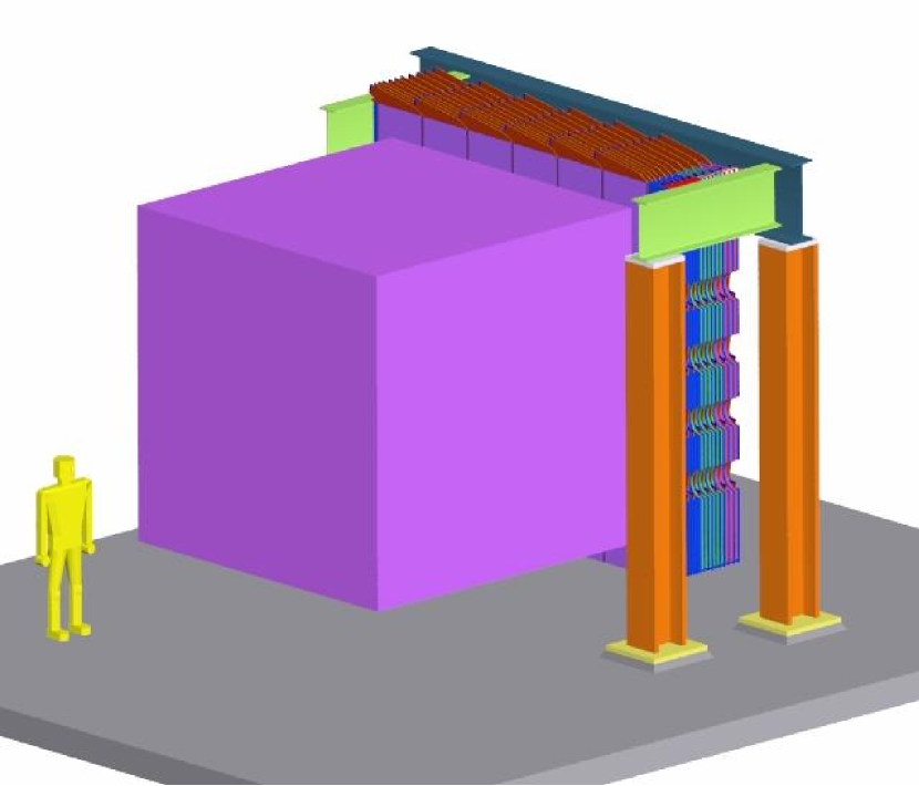
Figure 4.1: A schematic drawing of the FINeSSE detector. The cubic volume is the (3.5m)³ Vertex Detector. It is a (2.4m)³ signal region surrounded by a veto, filled with scintillator oil. The larger volume downstream is the Muon Rangestack.

4.1.1 The Vertex Detector

The FINeSSE Vertex Detector consists of a cube-shaped volume of liquid scintillator with dimensions $2.4\times 2.4\times 2.4$ m³. Light generated by ionizing particles traversing the scintillator is picked up by 1.5 mm diameter, WLS fibers, submerged throughout the sensitive volume. The fibers are mounted on a support frame, and are connected on one end to multi-anode photomultipliers, mounted to the outside of that frame. The fiber frame, photomultipliers, and associated electronics form a unit; this unit is immersed in the liquid scintillator, which is contained in a cubic tank, 3.5 m on a side. The volume between the fiber structure and the tank wall is used to monitor charged particles entering and exiting from the tracking volume (”veto shield”). The photomultiplier signals are processed in situ and transmitted by Ethernet to the outside of the tank, thus minimizing the number of cables that penetrate the tank wall. A schematic drawing of the tracking detector is shown in Fig. 4.2. Cables penetrate the tank wall above the oil level to prevent leaks.

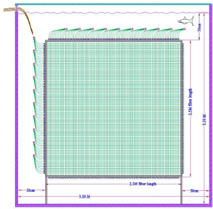
Figure 4.2: A schematic drawing of the Vertex Detector shown from the side.

Particle tracks can be reconstructed because the time of arrival of the light at the end of a fiber from a given source inside the detector is a known, continuous function of the distance between the source and the fiber. The detector will be calibrated using cosmic rays.

The arrangement of the WLS fibers is shown schematically in Fig. 4.3. There are three sets of fibers, running parallel to the axes of a Cartesian coordinate system. Except for a rotation in space and an offset, the three fiber sets are identical, consisting of fibers that intercept the wall at the vertices of a quadrate grid. The distance between grid points is 30 mm. Thus, the closest distance between any two fibers in the full assembly is 15 mm. The resulting arrangement is invariant with respect to a rotation by $90^{\circ}$ about any major axis. For the given dimensions, there are a total of $80\times 80\times 3=19200$ fibers.

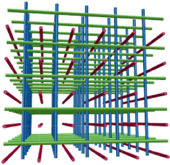
Figure 4.3: The geometrical arrangement of WLS fibers inside the Vertex Detector. The arrangement consists of three orthogonal sets of parallel fibers. The geometry is symmetric with respect to a rotation by 90^∘ about any of the three major axes.

Tracking Scheme

Consider a point source of light at some distance $d$ from a long, WLS fiber. A fixed fraction of the light that intercepts the fiber is wavelength-shifted and transported to the photo detector. Ideally, the exiting light is proportional to the diameter of the fiber and inversely proportional to $d$. In reality, this distance dependence is faster than $1/d$, because of light attenuation in the scintillator, and because the fraction of light captured by the fiber depends on the angle between the fiber and the incident ray.

The light collection efficiency versus distance to the fiber can be determined by Monte Carlo and test measurements. This dependence will be the same throughout the detector volume, with the possible exception of regions close to the wall, where reflected light may contribute.

The light from the source travels to all nearby fibers through a completely homogeneous medium. Since the sharing of light by nearby fibers can be used to localize the source, the position and angle of tracks can then be reconstructed. Fibers along a given direction are only sensitive to the projection of the track onto a plane perpendicular to that direction. Even if a second, orthogonal set of fibers is provided, it is still possible that a track may be parallel to one of two directions. This difficulty is avoided in the FINeSSE detector by having three orthogonal sets of fibers.

Light Generation and Transport

A comparative study of different scintillator fluids used in conjunction with WLS fibers is given in Ref. [55]. In general, an ionizing particle excites ultraviolet fluorescence ($\sim$ 350 nm) in the scintillator. This light is normally shifted to a longer wavelength ($\sim$ 430 nm), to avoid problems with absorption in the scintillator. The shifted light propagates isotropically. The light that intercepts a WLS fiber is shifted once more, to typically $\sim$ 500 nm to inject light into the acceptance cone of the fiber and to prevent re-absorption in the fiber. The WLS fiber consists of a polystyrene core (n=1.60), surrounded by cladding of a lesser index of refraction. The trapping efficiency of the fiber is significantly enhanced (to typically 6%) when two claddings are used. For a 1.5 mm diameter fiber, the first cladding is 45 $\mu$m thick acrylic (n=1.49), and the second is a layer of 15 $\mu$m thick fluor-acrylic (n=1.42). The data given here are for BCF-91A-MC fibers from Saint-Gobain [56]. Similar fibers are available from Kuraray [57]. The second cladding also provides protection against possible chemical interaction between the liquid scintillator and WLS fibers. Long-term tests of fibers in mineral-oil-based scintillation fluid, carried out in the context of MINOS R&D [58, 55], showed no discernible ill effects. Specifically, the BCF91A fibers used in these studies were not affected after having been suspended for six months, at temperatures up to 50^∘ C, in mineral-oil-based scintillator, BC517L, or in the high fluor concentration BC517H. Furthermore, single clad fibers suspended in B517L for more than two years also showed no aging or deterioration [55].

The attenuation length of the light propagating in the fiber is given as 3.5 m by the manufacturer, but a more complicated behavior is reported in the literature [55]. The attenuation length is the same whether the fiber is in liquid scintillator or in air [59]. Because of attenuation in the fiber, the light collected at one end depends on the point of origin along the fiber. This effect can be reduced by applying an aluminum reflective coating at the other end [60], or even by just painting it white with TiO₂ [55]. These coated fiber ends will be covered with a Teflon sleeve and will not be in contact with the mineral oil. Even in the case that they would, these coatings are inert and unlikely to interact with the scintillator oil.

We are currently investigating a number of options concerning the liquid scintillator. It is true that the present tracking scheme makes use of the sharing of light from a given source by a number of fibers. However, it is also true that only fibers in the vicinity of the track contribute significantly to the determination of the track parameters. As a result, low-attenuation length oil may be the best choice, which is an unusual but easily accommodated need. We are continuing R&D on the best choice of scintillator oil.

Advantages of the Proposed Design

Our design represents a novel approach to the task of tracking ionizing particles in a large-volume detector. It exploits the fact that the response of a fiber versus the distance to the light source inside the detector volume is a universal function, and the three-fold symmetry makes the tracking sensitivity nearly isotropic. These properties are particularly important for the physics goals of the present proposal. To our knowledge, there is no other scheme that offers these features.

We investigated an alternative detector design which consists of planes of bars of solid scintillator, oriented normal to the beam direction ($z$). Bars in even layers would run in the $x$ direction, those in the odd layers in the $y$ direction. Scintillating plastic bars are extruded polystyrene with $2$cm$\times 1$cm cross section. Each bar is co-extruded with a TiO₂ outer layer for reflectivity and a hole down the center for a WLS fiber. This design is very similar to the K2K scibar detector recently commissioned [61] and to that employed by the MINOS experiment [63].

Such a design for the Vertex Detector has a number of disadvantages for the FINeSSE physics goals. First, the tracking information would have to come from light sharing between several intercepted bars. The track resolution would therefore be limited by the bar dimension. Second, the amplitude information from a given bar reflects the overlap of the track with the bar cross section. Interpretation of this information is complicated and suffers from irregularities in stacking, caused by uneven extrusions and variations in the reflecting layer and in wrapping. Third, tracks that do not have a sufficiently large angle with respect to the stacking planes are lost. These disadvantages make reconstruction of low energy proton tracks and therefore low energy $\nu-p$ elastic events particularly difficult. Details of our studies of this design can be found in Appendix A.

Prototype Setup and Test Measurements

To demonstrate the viability of the proposed tracking scheme in the Vertex Detector, we have constructed and tested a prototype. The following contains a description of the prototype including construction issues and the results of beam tests.

The prototype Vertex Detector consists of a rectangular box made from anodized aluminum, $16\times 16\times 30$cm³ on the inside (Fig. 4.4), with a $6\times 5$ array of multi-clad, $1.5$mm diameter, WLS fibers (Bicron BCF-91A-MC, [56]). The fibers are spaced 20 mm apart, and penetrate the wall of the box. The fibers’ O-ring seals hold them in place, as will be done in the full-scale Vertex Detector (see Section 4.3). Light from the fibers is detected on one end by two 4$\times$4-anode photomultipliers (Hamamatsu H8711). The light-tight box is filled with liquid scintillator (Bicron BCS517H  [56]).

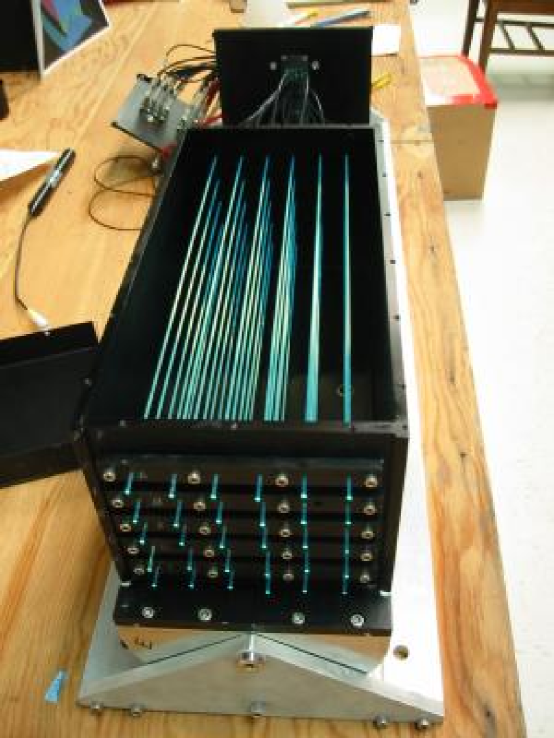
Figure 4.4: Photograph of the prototype detector with the mounted WLS fibers. The protruding fiber ends were covered with a light shield. The photomultipliers were mounted on the plate at the far end. The box could be pivoted to study beams that intercept the fiber matrix at an angle.

To test this prototype, the box was placed at the end of beam line I of the Radiation Effects Research Program (RERP) test station at IUCF [62]. A low-intensity, 200 MeV proton beam with a $6\times 6$ mm² profile (defined by two scintillators in coincidence) was aimed at the center of the box. Each passing proton produced a track with almost uniform energy deposition. The box could be moved vertically (henceforth called x-direction), or horizontally (y-direction) by remote control, enabling the beam position to be scanned perpendicular to or along the length of the fibers. The amplitude signals from all 30 fibers were digitized by conventional electronics and stored, event-by-event.

Light Yield Versus Track-to-Fiber Distance and Angle

With the box axis normal to the beam, a sequence of runs were taken, moving the beam from top to bottom in steps of 5 mm. For each fiber and each run, the centroid of the accumulated amplitude spectrum, corrected by its pedestal value, was determined. The centroid as a function of beam position is shown in Fig. 4.5. Before the centroid values were plotted, each fiber output was scaled by an individual gain factor such that all peaks lined up at an arbitrary centroid value of 100. The 30 fiber pedestals and gains thus determined were retained for the remainder of the test. This part of the test demonstrates that there is a universal law that governs the collected light as a function of the track-to-fiber distance.

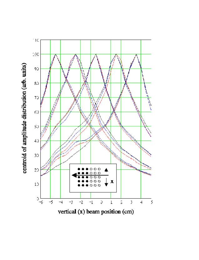
Figure 4.5: Normalized centroids of the light yields of 15 fibers as a function of the vertical beam position. The insert shows the position of the fibers plotted. The light yield is given in arbitrary units. To convert to units of observed photoelectrons, multiply by 0.17 (see text).

In order to study the angular dependence of incident light, the box was rotated around a vertical axis by an arbitrary angle ($\beta=27^{\circ}$), and the vertical scan, described in the previous section, was repeated. The result was virtually indistinguishable from Fig. 4.5, except for an overall scaling by $\frac{1}{cos\beta}$. This shows that the amplitude response of the detector is indeed sensitive to the projection of the tracks onto a plane orthogonal to the fiber direction.

Attenuation of Light in WLS Fibers

With a normal beam at constant height ($x=0.5$ cm), a scan along the fiber direction was carried out. For all fibers, we observed a light yield that slowly increased toward the end of the fiber that was coupled to the photomultiplier, with a sharp fall-off near both ends of the box. From the overall increase, we estimated a light attenuation length in the fiber of 150 to 200 cm. The fall-off at the ends is well explained by purely geometric arguments.

Absolute Light Yield

To absolutely calibrate the light yield, it is necessary to relate the photomultiplier amplitude to the number of collected photoelectrons (PEs). This can be done if the peaks that correspond to events with only one or two PEs are resolved. In the spectra obtained with the multi-anode photomultipliers this was not the case. We have therefore compared the tubes used in this test with a high-performance tube, using low-light pulses. We found that a track that intercepts the fiber (corresponding to 100 units in Fig. 4.5) yields an average of $17\pm 2$ PEs.

Reconstruction of the Track of a Single Event

In the following sections we describe an attempt to use a simple reconstruction algorithm to extract the angle and position of a track of a single event, and to determine the corresponding uncertainty. The track reconstruction algorithm used here is primitive but sufficient to prove the point. For instance, the simple algorithm does not take into account that the energy loss along the track through our test setup changes by about 40%. The track reconstruction algorithm used for the Monte Carlo sample for the entire FINeSSE detector, described in Chapter 5, accounts for these effects.

The observed dependence of the amplitude, $A$, on the fiber-to-track distance, $d$, (Fig. 4.5), is used to construct a function $A(d)$, chosen so it could be inverted analytically. Then, the amplitude data are converted to measured distances. In other words, for any given event $i$, the distances $d_{n,i}$ of that track from all fibers $(n=1-30)$ are known.

Fig. 4.6 shows the average distance of tracks from the top row, versus the average distance from the bottom row. Each event is represented by a point. The plotted events are comprised of 500 events from each of the runs of the vertical scan discussed above. As a result, the tracks to be analyzed more or less fill the space between the top and bottom rows.

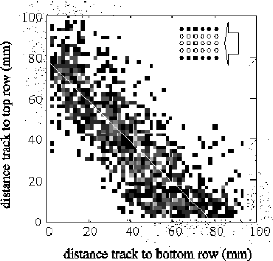
Figure 4.6: Distance to top row versus distance to bottom row, averaged over all six fibers in that row, for horizontal tracks that fill the space between the two rows.

Since the sum of the two distances equals the spacing between top and bottom row (80 mm), the events are expected to lie on a straight line. For the same events, Fig. 4.7 shows the average distance of tracks to the second row versus the average distance of tracks to the third row. For the tracks between the rows the sum of the distances is constant, as in Fig. 4.6 but for those outside the rows the difference must be constant. This can clearly be seen in the figures.

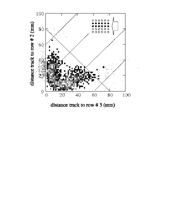
Figure 4.7: Distance to row 2 versus distance to row 3, averaged over all six fibers in that row, for horizontal tracks that fill the space between top and bottom row.

We parametrize a track by its position at the downstream face of the detector (the intercept with the $x$-axis) and its angle with respect to the $z$-axis. For a given event (track), the distances to all fibers are deduced from the measured amplitudes via the function $A(d)$, mentioned earlier. To reconstruct the track, one needs to find the straight line that is most consistent with these distances. This is accomplished by a regression algorithm minimizing the square of the difference between the calculated and the measured distance, weighted by the amount of light, summed over all fibers. In this way, one obtains the position $x$ and angle $\alpha$ for each individual track.

We have applied this procedure to 500 events of a run where the beam was normal to the fibers, and aimed halfway between rows 2 and 3. The expected position is therefore $x$=30 mm, and the expected angle is $\alpha$=0. In the reconstruction code it was possible to decide whether a given fiber should be allowed to contribute in the fitting procedure. The two panels in the top row of Fig. 4.8 show the reconstructed position and angle distributions when all fibers in the two rows on either side of the nominal beam position (a total of 24 fibers) are taken into account. The distributions represent a convolution of the intrinsic detector resolution and the phase space of the “beam,” which is defined by the trigger scintillators. In order to illustrate how this result depends on the number of participating fibers, we have repeated this analysis, taking into account only three fibers in each of the rows straddling the beam (a total of 6 fibers). The result is shown in the bottom row of Fig. 4.8.

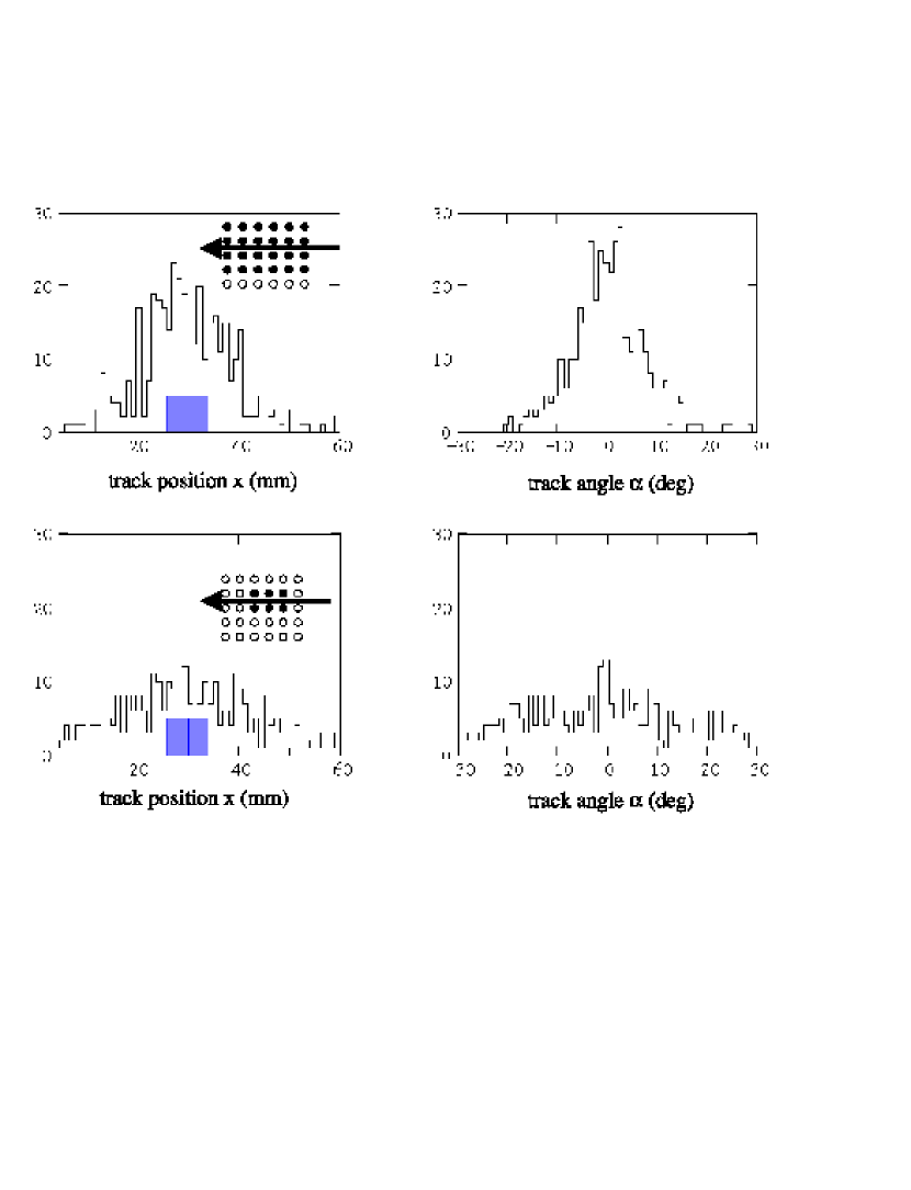
Figure 4.8: Reconstructed position and angle of tracks for two rows of fibers on either side of the beam (top plots) and for only three fibers on either side of the beam (bottom plots). The rectangular box in the left panels indicates the nominal beam position and width.

The measured track position and angle resolutions are dominated by statistical fluctuations in the number of PEs observed in the photomultiplier. This can be seen in the following way. Assuming a hypothetical track, and using the light-distance relationship $d(A)$ mentioned earlier, the signal amplitude (in arbitrary units) is calculated for all fibers. From the absolute yield calibration (100 amplitude units correspond to 17 PEs) we get the corresponding number of PEs. From a Poisson distribution with that mean, a random number is drawn to represent the “observed” number of electrons. This number is then converted back to amplitude units for all 30 fibers, and the resulting simulated event is reconstructed by the same algorithm used for the real events. As input, random tracks with $\alpha$ = 0 and 26.5 mm $<x<$ 33.5 mm (representing the beam width) were used. The simulated distributions for $x$ and $\alpha$ are shown in Fig. 4.9. Obviously, they are remarkably similar to the real distributions (Fig. 4.8), and since statistics is the only reason for smearing in the simulation, we conclude that this is also the case for the measured data.

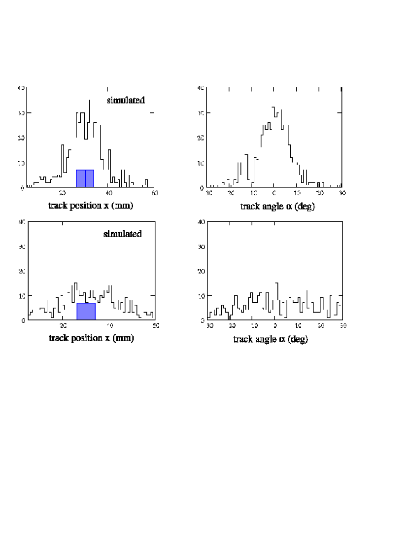
Figure 4.9: Simulated events, taking into account the Poisson statistics of the observed number of PEs (cf. Fig. 4.8).

Given the good agreement between real and simulated data, we can deduce the intrinsic detector resolution. We find that the position resolution achieved in our test is about 15 mm FWHM, and the angular resolution about 15^∘ FWHM. The difference between using 24 fibers and using only six fibers is not solely due to counting statistics. It is also affected by the fact that the length of the track, that is supported by distance information from the fibers, changes, thus relaxing the constraint on the track angles.

4.1.2 The Muon Rangestack

Downstream of the FINeSSE Vertex Detector is the Muon Rangestack. The Rangestack is designed to range out muons, in conjunction with the Vertex Detector, with energies up to 1.5 GeV, and to measure muon energy to 10%. These characteristics are needed to enable the reconstruction of charged current $\nu_{\mu}$ events, which are used in both the $\Delta s$ and the $\nu_{\mu}$ disappearance measurements. The Rangestack is located downstream of the Vertex Detector, because the muons from high energy CC $\nu_{\mu}$ events in the Vertex Detector tend to be produced at forward angles (See Section 5.2.2).

The iron absorber planes and tracking granularity in the Rangestack are designed to meet these requirements. The stack is comprised of $4\times 4~{}$m² planes of scintillator strips and iron absorber with an overall depth of 0.85 m (0.98 m including support structure) in the beam direction (referred to here as the z direction), and a weight of 100 t. Of the 0.85 m thickness, 0.24 m is scintillator and 0.61 m is iron. The design both meets the physics requirements and minimizes cost and space demands. The following sections describe the Rangestack’s design, construction, and readout.

Figure 4.10 shows isometric and orthographic views of the entire detector. The structural steel shown supporting the stack is a conceptual design. No PMT enclosures or clear fiber bundles surrounding the Rangestack are shown.

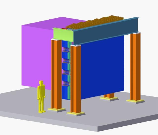
Figure 4.10: An isometric rendering of the Muon Rangestack in front of a box bounding the envelope of the Vertex Detector.

Advantages of Choosing a Rangestack Design

We have found that a Rangestack is the best choice to achieve our physics goals. The Rangestack is designed to range out muons, in conjunction with the Vertex Detector, with energies between 0.1 and 1.5 GeV. A stack of plastic scintillator bars interspersed with iron absorber is a relatively inexpensive and straightforward way to achieve these goals. This detector design has been well tested by the MINOS collaboration. They have shown that these plastic scintillator strips have excellent reflectivity, fast timing, simple design, long term stability, low maintenance and high reliability [63]. Furthermore, the expertise for construction and assembly of such a detector already exists at Fermilab.

A magnetic spectrometer was considered and rejected because it is very expensive compared to the Rangestack. Its obvious advantage – charge identification – is not necessary for the physics of the experiment.

Rangestack Design

The Rangestack consists of 21 pairs of a scintillating tracking plane and iron absorber. Each scintillating tracking plane is made up of 4.1 cm $\times$ 1 cm $\times$ 4 m extruded polystyrene scintillator strips. Each plane is oriented normal to the beam, with strips in the $x$ direction, in even numbered planes, and in the $y$ direction in odd numbered planes. The strips are arranged so that their depth in the $z$ direction is 1 cm. Each 4 m plane, then, contains 96 strips. The strips are packaged in groups of 16, surrounded by a 1 mm thick aluminum can for protection and light tightness. There are six cans of strips per $x$ or $y$ layer. Cans are identical between $x$ and $y$ layers, just rotated 90^∘ with respect to each other. The six cans in a layer are attached to a backing layer of 0.50 inch thick steel which serves to support the 4$\times$4 m² plane of scintillator and protect it during crane handling and shipment, and functions as part of the absorber layer between each $x$ and $y$ layer of scintillator. Figure 4.11 shows an assembled $x$ plane. Assembled $y$ planes are similar, with scintillator planes rotated by 90^∘.

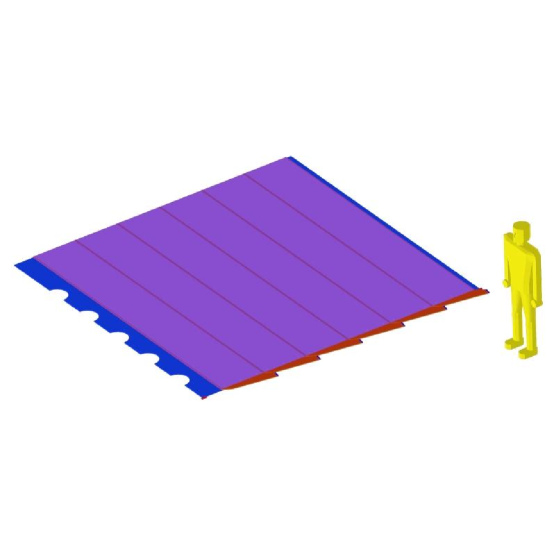
Figure 4.11: A completed $x$ layer with six cans of scintillator and a 0.50 inch thick steel backing. The assembly weighs 2.2 tons. Cans are attached to the steel backing by bolts at the ends of the can, and a strap (not shown) similar to the MINOS design which prevents the cans from bending away from the backing in the middle.

Scintillator strips in these planes are similar to those used in the MINOS experiment [63]. The scintillator is co-extruded with a TiO₂ outer layer for reflectivity. A groove down one side of the strip contains a glued-in-place WLS fiber. Light produced in the scintillator strips is absorbed by the WLS fiber and re-emitted at $\sim 500$ nm. Re-emitted light within the acceptance for total internal reflection is transmitted to the end of the fiber and detected by the phototubes, which are identical to those used in the Vertex Detector. The same type of WLS fiber will be used in the Rangestack and the Vertex Detector (see Section 4.1.1 for a description).

Interspersed with the active scintillator planes are iron absorber planes. In order to minimize the size of the Rangestack, the thickness of the iron in the absorber planes increases with increasing depth into the detector. This design is chosen to take advantage of the fact that once lower energy particles range out (leaving only higher energy particles), the iron absorber thickness can be increased while maintaining the same relative energy resolution. This is achieved easily by dividing the Rangestack into four sections with the thickness of the beam absorber increasing by 0.5 inches, or one iron plane, per section.

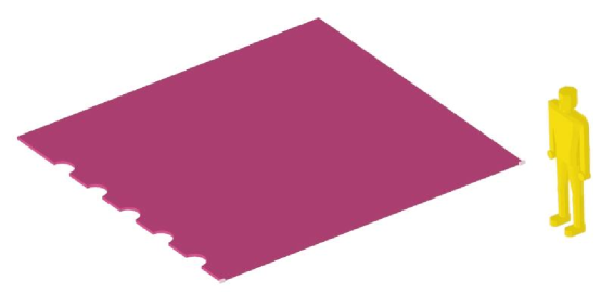
Figure 4.21: A typical filler module for section 4. Not shown on any of the module pictures are lifting lugs to place the modules in the stack. The ears that allow the plates to hang from the support structure are welded on tabs.

The upstream end of the range stack (section 1) has six layers, three $x$ and three $y$, with 0.50 inch total steel between layers. The backing plate for the scintillator planes provides this layer of absorber. Behind that is section 2, with six layers of $x$ and $y$ planes separated by a total of 1.00 inch of steel between modules. To make up the total thickness, there are 0.50 inch thick filler plates between scintillator modules. Section 3 has six layers of $x$ and $y$ scintillator planes separated by 1.50 inches of steel. Section 3 filler modules are 1.00 inch thick. Finally, section 4 has three absorber layers 2.00 inches thick, using 1.50 inch thick absorbers. An $x$ layer sits upstream of the first 2.00 inch thick absorber, followed by alternating layers of $y$, filler and $x$ layers. The stack ends with a $y$ layer. The final $x$ and $y$ layers in the stack are triple-thick to assure high efficiency for identifying stopped muons. Figure 4.21 shows a typical 1.50 inch thick filler module for section 4. The minimum thickness of 0.5 inches used in the first section of the Rangestack is set so as to ensure a 10% energy resolution for the lowest energy muons that enter the Rangestack.

Light Output and Readout in Active Rangestack Planes

Tracking planes in the Muon Rangestack must produce enough PEs at the readout PMTs to observe a Minimum Ionizing Particle (MIP) and therefore track muons. The scintillating strips, WLS fiber, and readout used in the Muon Rangestack are very similar to those used in the MINOS far detector. Light output from a Minimum Ionizing Particle (MIP) in the FINeSSE Muon Rangestack can be inferred from prototype testing results from MINOS.

As MINOS studies have shown, the efficiency for observing a muon crossing a strip is greater than 90% as long as at least 2.5 PEs are read out. In a prototype assembly of part of a scintillator plane for the MINOS far detector, a MIP passing through the center of a strip produces, on average, 6 PEs in total, with an average of 3 PEs read out on either side [63]. The design of the Muon Rangestack is such that there will be approximately twice this much light observed as a result of the differences between the MINOS strips and the FINeSSE Muon Rangestack strips. These differences in the design include the overall length of the strips, the WLS fiber size, and the fact that the readout takes place from one end only. The first two factors increase the light levels in the Rangestack by more than a factor of two as compared to the MINOS detector. The fact that readout occurs from only one end will decrease the light read out, but only slightly as reflective paint on the terminal end of the fiber will pipe light back toward the readout end.

WLS fibers are connected to clear fibers at the end of the scintillator strips as is done in the MINOS detector and as is shown here in the Muon Rangestack design. Clear fiber ribbon cable will then route the signals to the removable floor above the detector where they will be read out via the same system employed in the Vertex Detector as described in detail in Section 4.1.3.

4.1.3 Signal Readout: Phototubes and Electronics

We propose a common design of signal readout to be used for the Vertex Detector, its veto shield, and the Muon Rangestack. Requirements for the readout system include independent amplitude and timing measurements for each channel. The amplitude information is used in the track reconstruction and for $dE/dx$ measurement for the particle tracks; timing information is used to assemble the hits (rejecting spurious noise hits and background tracks), to correlate with the beam spills, and in the analysis of secondary events, such as muon decay and nuclear decay in the active volume following the capture of a neutron produced in the primary event. In the Vertex Detector the full scale signal range will extend to $>50$ PEs, with an amplitude resolution of $<0.1$ pe. The timing resolution is not crucial, but it needs to be $\sim$ 10 ns to reduce spurious hits and background tracks.

The readout must be sensitive both to the primary interaction events (which are in time with the beam spill) and to secondary events as described above. It is also useful that it be sensitive to cosmic ray muon tracks, for calibration purposes. For these reasons, the front end electronics must be self-triggering and have a relatively low deadtime after being hit. Deadtime of the proposed system is about $1-5\;\mu{\rm s}$, depending on signal amplitude (see discussion below). The deadtime applies independently to each channel – this is a matter of recovery of the front end electronics only, since there is zero deadtime associated with the data readout. A external global trigger will also be implemented, which can be used to force an event readout and/or a charge pulser event, for diagnostic purposes.

The readout system designed to meet these requirements combines multianode photomultiplier tubes (MAPMTs) and custom readout electronics in a 128-channel “readout module.” This includes two MAPMTs, front end electronics, HV bias circuits, charge-injection test pulsers, and data acquisition and control communications. The module is a sealed, conductively cooled unit suitable for submerged operation inside the oil tank (for the Vertex Detector application). In the Muon Rangestack the readout modules will be housed above the removable floor above the detector. The Vertex Detector requires 150 modules for readout of the active volume and six modules for the veto shield. The Muon Rangestack readout requires an additional 17 modules.

Multianode PMTs

Fibers from the Vertex Detector, veto, and Muon Rangestack are read out via Hamamatsu R7600-00-M64 MAPMTs. This multianode photomultiplier tube provides an $8\times 8$ array of optical readout in a 25.7 mm square by 20.1 mm deep metal package. We intend to operate the MAPMTs at a gain of $8\times 10^{5}$, which corresponds to a typical cathode supply voltage of $-875$ V. Channel-to-channel gain variation in the MAPMT is 5:1 maximum. As a result, if it is assumed that a channel in the middle of this ratio is set to the desired gain, the required full scale range of the front end electronics is $8\times 10^{5}\times\sqrt{5}\times 50q=14\;{\rm pC}$, and the required resolution is $(8\times 10^{5}/\sqrt{5})\times 0.1q=5.7\;{\rm fC}$, a dynamic range of 2500. The R7600-00-M64 MAPMT is similar to the sixteen anode R5900-00-M16 (see in Figure 4.13).

Front End Electronics

Continuously running commercial multichannel 10-bit pipeline A/D converter chips, such as the ST Microelectronics TSA1005-20IF, will form the heart of the FINeSSE front end electronics (FEE). One such converter will digitize signals from each anode of each MAPMT, at a rate of 20 Msamples/s. Since this sampling is, of course, significantly coarser than the MAPMT output pulse width, and significantly coarser than the desired time resolution of 10 ns, suitable analog signal processing before digitization, and digital signal processing after, will be employed.

The analog signal processing must shape the MAPMT output pulse so that it extends over several A/D converter samples (offering a chance to measure the amplitude), and so that it does something characteristic (such as have a peak, or better yet a zero-crossing) at a defined time after the MAPMT output pulse (offering a chance to measure the time of occurrence). In addition, the analog signal processing circuit must present a low and resistive impedance to the MAPMT anode, so that all the induced charge is swept quickly into the signal processing for that anode, and does not go into parasitic capacitances to ground or to other anodes. The simplest circuit which can achieve these things is an inverting op-amp with an RLC network in feedback. In response to a $\delta$-function current input, $I(t)=Q\delta(t-t_{0})$, a damped cosine wave is output, $V(t)=(Q/C)\cos(\omega(t-t_{0}))\exp(-\lambda(t-t_{0}))$ for $t\geq t_{0}$. The amplitude is proportional to the input charge, and the phase, or equivalently the time of the first zero crossing, is directly related to the time of occurrence of the input charge.

The required digital signal processing simply undoes the above. If $R$, $L$, and $C$ are known, then $\omega$ and $\lambda$ are known, and a simple linear fit of the measured data points to $V(t)=A\cos(\omega(t-t_{0}^{\prime}))\exp(-\lambda(t-t_{0}^{\prime}))+B\sin(\omega(t-t_{0}^{\prime}))\exp(-\lambda(t-t_{0}^{\prime}))$,where $t_{0}^{\prime}$ is the time of the first ADC sample found above threshold, determines the amplitude and the relative time $t_{0}-t_{0}^{\prime}$ of the input pulse. Of course, there will be manufacturing tolerances on the component values, and potentially a small drift with time or temperature. To calibrate these, a nonlinear fit involving $\omega$ and $\lambda$ as parameters is performed occasionally.

The number of raw A/D samples to be used, and the desired value of $\omega$ and $\lambda$ of the filter, needs to be carefully optimized. In particular, the response should decay to less than a few percent within $5\;\mu{\rm s}$. A following pulse which occurs within 5 $\mu$s can still be measured, provided that the amplitude of the waveform does not exceed the range of the A/D converter. The actual deadtime for a full scale amplitude pulse following another full-scale amplitude pulse may be as large as 5 $\mu$s, but for pulses of smaller amplitude, e.g., less than half-scale, the deadtime can be as small as 1 $\mu$s or even 800 ns. For pulses separated by less than that, it is still possible to discriminate that there is a second pulse, by applying a threshold to the $\chi^{2}$ of the fit, even if it is not possible to estimate the amplitudes and times separately. The low deadtime and double-pulse discrimination capability is important to detect muon decay events, both for particle identification and as a method of gain calibration.

An important difference from the conventional approach, where a discriminator and dedicated time-to-digital converter are used, should be noted. Conventionally, the discriminator is set to respond to the first, or at least the first few, PEs in the signal, and thus the measured hit time is insensitive to the later PEs. As a result, the measured hit time is more accurately related to the time of the charged particle passing in the detector. In the present approach, where a timing discriminator is not used, by contrast, the measured hit time depends on all the PEs in the signal. This will not yield as good a result; nevertheless, because the scintillator oil and wavelength shifting fiber both have short decay times (2 ns for the oil, 3 to 10 ns for the WLS fiber), we can achieve the required 10 ns timing accuracy.

The digital signal processing will be performed by a combination of field programmable gate arrays (FPGAs) and a microprocessor (also used for communication and control – see below). The FEE FPGAs, handling 8 or 16 channels each, will monitor the digitized data from each channel, apply the trigger threshold, capture the required number of data points after seeing the threshold crossed, and send them to the microprocessor. There the linear fit calculations are performed, and the amplitude and time thus determined are queued for transmission to the DAQ.

This front-end electronics design for FINeSSE is intended to take maximum advantage of low cost commercial electronics to provide a highly parallel measurement of pulse amplitude and timing with minimal deadtime. Although there are ASICs such as the VA-TA series from IDE, Inc. which have been applied to very high density readout electronics for MAPMTs, none of the presently available ASICs can match the low deadtime performance of the system described here when the hit patterns are non-sparse as in the FINeSSE Vertex Detector. Furthermore, FINeSSE does not strictly require such very high density electronics, since each MAPMT covers a 240 mm $\times$ 240 mm area on the detector, making almost that much area available for the readout electronics. In any case, with the large commercial market driving down the costs of pipeline ADCs and FPGAs, the proposed approach can be more cost effective.

An independent charge-injection test pulser will be included on each channel. This diagnostic feature will be useful in testing the front end electronics and the readout, and debugging the system during operation.

The Readout Module

The readout module is comprised of two Hamamatsu R7600-00-M64 MAPMTs described in Section 4.1.3, a high voltage bias generator, 128 channels of front-end electronics, a microprocessor, a data network interface, a system clock and trigger interface, and a power supply. (See the block diagram in Fig. 4.12.) The microprocessor handles control and housekeeping tasks, data transmission tasks, and also the fitting algorithm (described above) to calculate the hit time and amplitude based on the raw ADC samples captured in the FEE. Normally only the time and amplitude will be sent to the DAQ, although for calibration of the algorithm above, the raw samples will be sent on selected events.

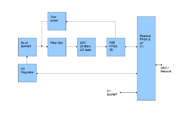
Figure 4.12: Block diagram of the readout module.

The module will perform zero suppression based on a programmable amplitude threshold. This threshold is independent of the trigger threshold used in the FEE to detect and capture an event. Note that both thresholds are applied digitally and can easily be set on a channel-by-channel basis, which can be helpful in dealing with any hot channels.

The module can also be programmed to suppress data not satisfying a pattern cut. For instance, a requirement of $\geq 2$ hits within a 20 ns window will almost completely suppress MAPMT dark pulses, even with the trigger threshold set very low, without adversely affecting real events. More complex cuts, such as requiring a track through the contiguous fibers of the module, can be imposed as well, although a cut requiring data from other modules would need to be imposed in the DAQ computer, since the event data will not be communicated directly between the modules. (Each module reads out an $8\times 16$ array of fibers on one face of the detector.) Note that the front-end electronics will process every hit seen on every channel; both the zero suppression and any other cuts that may be programmed into the readout module act on digitized data before transmitting it to DAQ, and the purpose is only to reduce the volume of unwanted data.

The output data from the readout module will be, for each hit, a 32-bit coarse timestamp from a counter, 8-bit fine time, and 12-bit amplitude. For data budgeting, we assume here that each of the latter will be embedded in a 16-bit word, which may include some extra “status bits.” (If data volume or data rates become an issue this could be revisited; also the 32-bit coarse timestamp could be compressed easily, since the relative time between subsequent transmitted hit data in general will not require 32-bit representation.) At 8 bytes per hit, the worst case event, where all channels of a module are hit, will generate 1.02 kbytes of data to be transmitted to the DAQ. An elasticity buffer of 16 kbytes or greater will be implemented in the module to allow for bursts in the incoming data and other network activity such as packet re-tries and control transactions.

Estimated power dissipation of the readout module is 20 W (156 mW/channel). The power input will be from a single 24 to 48 V DC supply. Each module will have an individual power cable from a fused power distribution panel outside the tank. In this way a module with a catastrophic power short can be easily isolated to allow the others to continue operation. High-reliability steering diodes will direct the input voltage to one of two independent fully isolated DC/DC converters in the readout module, based on polarity. The outputs of these supplies will be connected through further steering diodes. In this way we obtain the benefits of two almost fully independent power systems in each module, with no overhead for additional cables or connectors. Fully isolated DC/DC converters are required anyway, so that the modules can be powered from a common DC source and still have equal ground voltages, which simplifies the data network requirements (no AC coupling or wide common-mode transceivers are required). The internal circuitry of the module will work largely from a single $+2.5$ V supply (about 4.5 A), with an auxiliary $\pm 3.3$ V supply for some functions, and another auxiliary $-1050$ V supply for the MAPMT bias circuits. HV will be regulated to each MAPMT individually through a high-side pass transistor driven by an analog optoisolator. This will feed a conventional resistive voltage divider for the dynode string. A Cockcroft-Walton type of PMT bias circuit will be evaluated as an alternative, for reduced power, but reliability is likely to be greater using the resistive divider circuit.

The microprocessor and the data network interface are also potential single-point failures affecting an entire module. We will carefully evaluate a redundant system design around the microprocessor and its boot EEPROM in particular. We expect to implement a redundant network (pair of networks) for each of the five logical networks (described below); in particular an unpowered module shall be positively disconnected from the data (and clock) networks. Even when powered, it will be positively disconnected from the primary data network unless a watchdog timer is kept alive by properly functioning software. Download of new code shall be possible via either network, even if the old contents of the boot EEPROM are corrupted. (In particular the network disconnection watchdog may be defeated until a defined time after power-up.)

With proper attention to the above details, reliability of the modules can be assured to a degree which will allow them to be mounted in the inaccessible interior of the oil tank. The costs involved in this redundant design are significantly less than would be involved in transporting either the scintillation light out of the oil tank on optical fibers, or the anode signals from MAPMTs mounted in the oil tank to readout electronics outside. Remaining single-point failures, except in the MAPMTs or the divider resistor string, can affect at most eight channels.

The power-dissipating electronic components in the readout module will conduct heat through their leadframes or other thermal bonds into the extra thick (2 oz.) copper ground plane of the printed circuit boards. The printed circuit board ground planes are directly tied to the the outer aluminum case of the module, either by wedge-lock clamps or simply by screws and aluminum frames. Temperature rise between the module case and the printed circuit board ground planes will be about 5 - 10 K. Scintillation oil circulating in the Vertex Detector will cool the readout modules. The total heat load into the oil is $156\times 20\;{\rm W}=3.1\;{\rm kW}$, which can be removed by circulating the oil through an external water-cooled heat exchanger at at least 8 gal/min, assuming a 5 K temperature rise. The 17 readout modules of the Muon Rangestack will be cooled by fans mounted externally to their cases. All the modules will have internal temperature monitors and a hardware overtemperature interlock.

The readout module will be constructed as a black anodized aluminum box with an oil-tight gasketted lid. Attention will be paid to minimizing enclosed or recessed spaces in the outer surface of the box, the screws and other hardware, and the connectors and cables; furthermore the box will be purged with nitrogen internally after assembly. These measures should minimize the contamination of the scintillating oil with oxygen, which can degrade the light yield.

Network, Data Acquisition System, and Clock and Trigger Distribution

The 173 readout modules in the system buffer data internally, and communicate it, as needed, to the data acquisition computer system over a serial multidrop bus architecture. Although other implementations, in particular 10 Mbit/s Ethernet or CANbus, will be considered carefully at the design stage, at the time of this writing we assume a synchronous serial bus (separate data & clock lines) implemented with RS-422, running at 2 Mbit/s, using HDLC (High Level Data Link) protocol. For acceptable bus loading the readout modules will be arranged in five networks of up to 39 modules each (four used for the Vertex Detector and a fifth for the Muon Rangestack). The DAQ computer will be a Linux box with two DMA-capable PCI quad RS-422 communication controller boards installed. These are expected to be commercial off-the-shelf devices. Control and status communications will run over the same networks as the readout data.

With 10% overhead for protocol the worst case module, with 1.02 kbytes of data, will require 5.6 ms for data transfer. Furthermore, assuming that the networks are physically arranged to balance the data load, each will see typically up to 250 hits per spill, which is 2.0 kbytes of data. Since this is coming from 39 different nodes, assume a 100% overhead for protocol. (In actuality the data is buffered in the readout modules, so not every module will send a data packet on every spill, but for a reasonable worst-case estimate we ignore that here.) Then the complete data transfer on the network requires 20 ms (this includes the up to 5.6 ms for the worst case module). Since the spills are 66 ms apart, there is adequate spare capacity to accomplish this.

The overall data rate into the DAQ computer, 16.6 khits/s = 133 kbytes/s, will be quite manageable, for transfer over the PCI bus, online monitoring software, and local disk storage or TCP/IP network transmission.

The 32-bit coarse timestamp provided by the readout module rolls over in 429 seconds. Therefore the DAQ computer will augment this timestamp with further bits to provide an absolute time measurement without rollover.

A 10 MHz reference clock and global command word are distributed to the readout modules over separate, but similar, serial multidrop networks. The global command word is used to synchronize the timestamp counter of all modules, and to fire the global trigger and test pulser events as described above. The serial communications network clocks will also be derived from the same 10 MHz clock for convenience. The reference clock will be provided from an oscillator module which may either be a standard crystal oscillator or an absolute GPS-referenced timebase.

Heritage

Indiana University Cyclotron Facility personnel have significant recent experience designing and constructing a 9216 channel MAPMT readout system for the STAR Endcap Electromagnetic Calorimeter shower-maximum detector [64]. Figure 4.13 shows a picture of the R5900-00-M16 MAPMT together with the Cockcroft-Walton base and front-end electronics. The front-end electronics for STAR uses switched-reset gated integrators and 12-bit pipeline A/D converters to provide a 12-bit integrated amplitude measurement for every channel for every bunch crossing time (period of $\approx$ 103 ns) in the RHIC ring. Data is stored until an external trigger decision, and then all 9216 channels are read out in less than 20 $\mu$s. The readout is modular in groups of 192 channels (12 MAPMTs); the modules being enclosed in rugged, magnetically shielded, water-cooled steel boxes which bolt to the STAR magnet poletip. While in functional details the system proposed here differs considerably from the STAR readout, many aspects of the design (such as the pipeline A/D converter and FPGA circuits, the conductively-cooled printed circuit board designs, the choice of connectors and other components, and test and diagnostic procedures) will either carry over directly or be informed by the lessons learned in the STAR readout work.

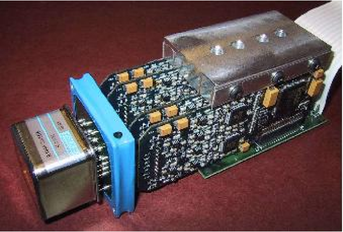
Figure 4.13: MAPMT (16-channel), Cockcroft-Walton base, and FEE assembly developed at IUCF for the STAR experiment at BNL.

4.1.4 Calibration

The FINeSSE calibration system must calibrate the response of the MAPMTs of the fiber network to light from charged particles in the scintillator. It must also calibrate the energy response of the tracking detector. The relative gains of the muon range stack scintillator strips must also be understood.

To calibrate the response of scintillating fibers and MAPMTs, FINeSSE will utilize cosmic ray muons and their Michel decay electrons. The energy distribution of Michel electrons is well defined and provides a “standard candle” for the calibration.

The veto fibers alone can be used to trigger on through-going muons. By using the veto and tracker sections, a cosmic Michel decay trigger can be set up. The cosmic muon events will put a known amount of light into the detector volume, with the geometry of the tracks constrained by the veto section, allowing accurate checks of light production by muons in the detector. The Michel events will provide enough low level light to calibrate the charge response of the fibers and photomultipliers. They will also provide a good sample for $\frac{dE}{dx}$ reconstruction calibration.

The muon range stack will also be calibrated using cosmic ray muons. The primary goal is to calibrate the relative gains and efficiencies of the scintillator strips. This should be easily achievable with the high rate of cosmic muons that FINeSSE will see. The calibration procedures using muons and Michels will be developed using Monte Carlo events.

4.2 Detector Location and Enclosure

The FINeSSE detector will be housed in a below ground enclosure 100 m along the line connecting the Booster neutrino production target and the MiniBooNE detector. Figures 4.14 and  4.15 show a side and top view of the detector within the enclosure. A detailed study, cost estimate, and schedule for this enclosure, performed by FESS, can be found in Appendix B.

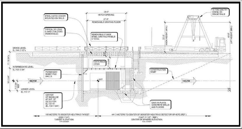
Figure 4.14: Side view of the 25 ft below grade detector enclosure to house the FINeSSE detector.

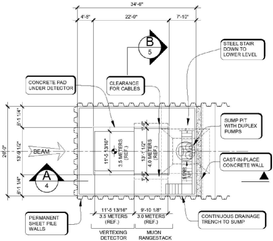
Figure 4.15: Top view of the detector enclosure.

The detector is installed using a gantry crane, above the enclosure, to move detector components from a truck, down through a removable hatch to the enclosure floor. The hatch can be rolled in and out of position on a daily basis to accommodate changes in weather and therefore in the installation schedule. Once installation is complete, shield blocks are installed above this to reduce cosmic ray rate in the detector.

The detector is accessible via a staircase with landings at a floor above the detector and at the bottom of the enclosure. The floor above the detector holds electronics racks and computing needed for readout, triggering and monitoring. Ethernet from both detector sections is fed through the removable floor to these racks.

Temperature control is minimal as per the requirements of the detector. Temperature of the Vertex Detector is controlled by a standard oil temperature control system like that used in the MiniBooNE experiment [65]. Temperature control of the electronics racks is done by enclosing them in a caboose and cooling or heating the caboose as necessary.

This detector enclosure is minimal, but it is practical and fulfills our needs. We have studied the feasibility of a below-ground enclosure in detail and in conjunction with FESS. A similar enclosure constructed of sheet piling with a removable roof housed experiments at PC4. A senior FINeSSE scientist examined this PC4 enclosure for toads, raccoons, and mice, and concluded this design will be sufficient.

4.3 Detector Fabrication and Installation

Detector components will be fabricated at Fermilab and FINeSSE collaborating universities. Components will be assembled at a staging area before installation in the detector enclosure. Lab E or the New Muon Lab at Fermilab would be a suitable place for this staging area. Because the enclosure is below ground, the goal is to minimize the actual construction at the site. Subdetectors are constructed in large “packages” with outer protection. What follows is a description of fabrication and assembly for the Vertex and Rangestack components of the detector.

4.3.1 Vertex Detector Assembly

The detector assembly is constructed as a unit, at the FINeSSE staging area on site. Once assembled, it is moved to the FINeSSE enclosure and craned into position. Engineering of the transport is underway. Finally, the scintillator tank is filled with scintillator oil. The Vertex Detector assembly is described below.

The main component of the detector is a cubic structure of six identical grid panels. Each of these is comprised of a stainless steel angle frame and an 80$\times$80 array of interlocking thin stainless steel ribs. These ribs are notched and positioned at an equal spacing of 3 cm, welded together at each intersection and to the frame around the perimeter. Each grid panel is constructed with the ribs centered with respect to the frame in one direction, and offset by 1.5 cm in the other. Mounting fixtures position the panels so that alignment may be made to assure that positions of the grid intersections are accurate and orthogonal throughout the cube. The offset directions of the panels are rotated so that any one direction of grid and the resulting fiber array is centered with respect to the other two directions.

The fibers are held in place by riders on the intersections of the grid (see Figs. 4.16 and 4.17). The riders are spring-loaded, providing a tension of 1 N per fiber. The deformation by the combined pull of 6400 fibers of a $2.5$m by $2.5$m grid plane, supported on the edges, is about $1$mm in the center.

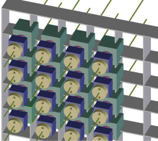
Figure 4.16: Supporting grid for the WLS fibers. Shown are the riders (slotted cubes) and the locking mechanism, which is pushed away from the rider by a spring.

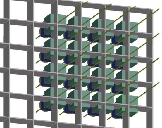
Figure 4.17: Same as Fig. 4.16, but seen from the inside of the fiber volume.

The fibers will be mounted in the completed support structure (after all six sides of the structure have been joined to form a cube). For mounting, an insertion tool is needed that can hand a fiber end to the opposite side of the cube, reaching through a partly occupied grid cell. It is conceivable to do this with a group of fibers simultaneously. Once the fibers are available at both sides, the riders are put in place. Once set up, we estimate that the mounting takes on the order of a minute per fiber. This amounts to about 10 weeks (assuming 8 hours/day and 5 days/week) for the fiber assembly.

The weight of the support structure is about 2 tons. This does not include the 330 MAPMTs with associated electronics, which are mounted on the outside of the fiber support structure. When routing the fibers from the riders to the tubes one must take into account that the minimum recommended bending radius for 1.5 mm diameter fiber is 12 cm. The section of fiber outside the support lattice and the tubes are encased in light-tight Teflon sleeves.

Once fiber stringing is complete, the electronics module support is put in place, the modules are mounted and PMTs plugged in, and each of the 300 ’cookies’ are locked to their PMT with spring loaded mountings. Cables suitable for submersion in scintillator oil are connected to the electronics modules.

The completed fiber structure will be lowered into a tank which will eventually contain the liquid scintillator. This outer tank provides a cubic volume, 3.5 m on its side. The fibers exit the top of the tank. Equipment to detect light from the veto shield, i.e., the volume outside the fiber cube is mounted along the walls of the tank.

The assembly is protectively enclosed and transported to the experimental location by a truck able to move 5 tons with a maximum tilt of 5^∘ and acceleration of 0.5 g. The onsite crane removes the detector from the truck and lowers it in place where fixturing assures its proper position. The hatch to the detector hall is then closed. The remaining veto area monitoring equipment is installed and cables from all electronics modules are routed to feedthrough panels. After all electrical connections are tested, the lid is put in place and the detector is filled with scintillator oil.

The system for circulation and temperature control of scintillator is then put into operation, as is the system for maintaining the nitrogen atmosphere in the tank above the scintillator. The liquid is circulated by feeding from the top back to outlets distributed around the bottom of the tank. The circulation is necessary to control the temperature of the liquid, and to de-oxygenize the liquid scintillator initially (resulting in a gain of about 25% in light yield). The tank has a gas-tight lid, in order to maintain an oxygen-free atmosphere above the liquid. The cables from the electronics readout modules in the liquid exit the tank through gas-tight ports above the liquid level.

Temperature of the submerged PMTs and electronics is controlled by a system which circulates and cools the oil. Additional PMTs and electronics monitor a veto region surrounding the six sides of the detector active volume. Electronic cables are routed to feedthrough panels along the upper surfaces of the walls of the tank above the oil level, where a clean nitrogen atmosphere is maintained during the operation of the system.

4.3.2 Muon Rangestack Assembly

For the Muon Rangestack, we must consider fabrication of the steel absorber and the scintillator hodoscopes. Fabrication of the pieces will occur at a Fermilab facility away from the detector site. Then the modules will be transported to the detector hall.

The steel will be procured by competitive bid from commercial machine shops and steel vendors. The absorber will have to be welded together from smaller readily available plate sizes, then cut to final size. No attempt has been made here to show the plate segmentation, as that will undoubtedly be determined by each steel vendor and the exact configuration of weld seams is irrelevant to the operation of the detector. Finished plates would be shipped to FNAL by truck. The route will have to be planned carefully, as will the fixturing on the truck, as these will be oversize loads. Calculation has shown that the plates can be rotated from a horizontal to a vertical position by pivoting them on the lower edge without exceeding the yield strength of the steel. However, once scintillator cans have been installed, a lifting/rotating fixture will probably be needed. Section 4 filler modules weigh 5.72 tons, and are the heaviest single pieces to lift. This puts a lower limit on the building crane in the assembly area at 6 tons, probably 10 tons when fixtures are included.

There are 2112 scintillator bars to be extruded, cut to length and staged. These could be extruded at Fermilab [66]. After cutting and finishing the ends, WLS fiber of the appropriate length will be laid in the groove and glued to the bar. The fiber gluing operation can be done after the bars are glued into the can bottoms. Large tables at least 4.6 m long will be used for curing the glue between the bars and fibers, and cans and bars. With staging areas, the floor space available should be at least $10\times 10$ m². Machines for mixing glue, applying it, and laying the fibers will be needed.

The MINOS TDR showed the aluminum cans which will hold the scintillator as made on-site from coils of 3003 aluminum sheet 0.040 inches thick [63]. A rolling machine was used to flatten the coils, and then to put corners along the edges used for crimping the lower and upper sheets together. We will have to examine the economics of this process, as having finished pieces delivered from a vendor may be more cost and time effective. The 4 m long pans are no problem for delivery by truck. 132 bottom cans and 132 top plates will be made.

The PVC spacers and fiber routing manifolds are very straightforward machined parts that can be fabricated at any machine shop equipped with CNC milling machines. PVC is stable after machining and relatively cheap.

Clear fiber bundles with their connectors must also be assembled, glued, and finished. Care must be taken to appropriately label fibers to assure that connections between scintillator cans and PMTs are correct.

Assembly of the can proceeds as follows. The set of scintillator strips are glued to an aluminum skin to hold them fixed, and then placed within a can. The WLS fibers are routed through grooves milled into a PVC plate at the end of the can. The plate forces the fibers into their recommended 12 cm bend radius and prevents them from being damaged during handling. The plate is glued into the can and light-sealed with a cover plate of PVC plastic. An optical connector is also attached to the grooved PVC plate. This connector joins the WLS fiber to clear fibers that go to the PMT enclosures. The construction technique follows Chapter 5 of the MINOS TDR [63], with the aluminum skins crimped at the edges to enclose the scintillator.

An exploded view of the fiber routing components is shown in Figure 4.19. Figure 4.18 shows a rendering of a can without the final light-tighting layer of aluminum over the strips. The PVC cover is also not shown. The schematics do not show the clear fiber bundles, the PMT enclosures, and the clear fiber.

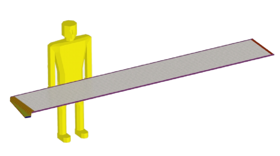
Figure 4.18: A can of scintillator strips with WLS fibers and enclosing PVC and aluminum sheet weighs just under 100 lbs and is approximately 4.3 m long including the PVC plates for protection of the fibers out to the optical coupling.

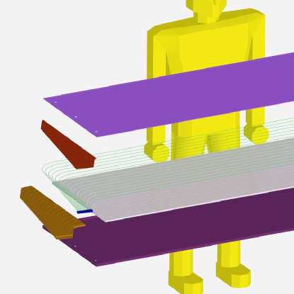
Figure 4.19: An exploded view of the end of the can that routes fibers to the optical coupling.

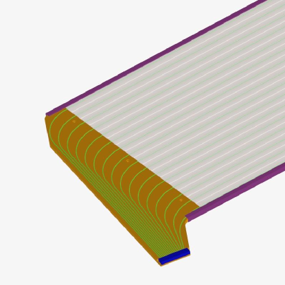
Figure 4.20: A close-up of the fiber routing plate at the end of the scintillator can. Not shown are the cover plates that light-tight the assembly.

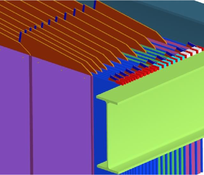
Figure 4.22: Close-up of the support rail showing the ”ears” on the steel plates that allow the plates to hang from the rails. The column and cross member at this corner were turned off to show more details.

Once scintillator cans are complete, their light tightness and other performance features may be tested. This is one of the big advantages of the 16-fold packaging of the scintillator. Cans are much easier units to handle for movement around the assembly area and for testing than full planes.

Finished cans will be attached to 0.50 inch protective steel backing plates at the assembly factory. Fixtures for vertical storage will be necessary. Finished scintillator planes weighing 2.2 tons and being about 15 feet square will be trucked to the detector installation site.

At the detector site, each module sits between two support rails upon which the Rangestack hangs, as indicated by Figure 4.22. The rails must be far enough apart to clear the ends of the scintillator can optical connectors. The protective steel backing, which is wider than the scintillator cans, is attached to each module. The steel backing is designed to protect the optical connectors during lowering into the stack. These plates are designed with scalloped edges to allow access to the clear fiber bundle, connector, and fastener exiting the side of the detector ($y$ view; Figure 4.23) once the module is in place.

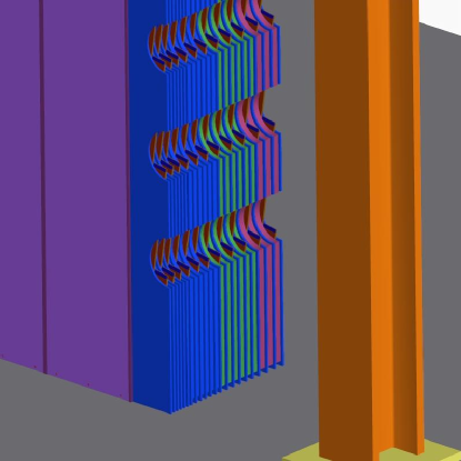
Figure 4.23: Close-up view of the changing thickness of the layers from section to section, and the scallops allowing access to the optical connectors on the $y$ planes. This face will probably also have structure to support PMT boxes and catwalks for maintenance access.

Because $4\times 4$ m² plates are larger than commercially available plate stock, this design assumes that a 4 m square plate will be welded together from smaller plates, and water jet or plasma cut to final shape. Figure 4.22 shows a closeup of the ears on the steel plates that support the scintillator and filler modules. Figure 4.23 shows a closeup of the side of the detector with the $y$ optical connectors and the scalloped steel edge.

Once all scintillator planes and absorber fillers are completed, they will be transported to the detector site. MI-12 or MI-8 will be used for temporary storage at the site. For installation, each module will be made vertical (if they are not already on the truck) and lowered into the detector pit to hang on the two support rails. The scintillator planes will require a simple beam lifting fixture to prevent excessive deflection during crane handling operations.

After installation of planes, the surrounding PMT boxes and support structure will be assembled. Clear fiber bundles will then be connected and testing with cosmic rays can begin. This can proceed with the building roof re-installed.

Chapter 5 Event Simulation, Reconstruction, and Analysis

The detector and physics events have been simulated and reconstructed to determine the feasibility, strategy, and sensitivity of the experiment for its two main physics goals: a measurement of $\Delta s$ and $\nu_{\mu}$ disappearance. In this chapter the general features of the neutrino interactions and tracks in the detector are described. Next, the detector simulation and reconstruction programs and strategies are explained. Backgrounds, both beam-related and beam-unrelated are then discussed. In the final part of the chapter, the methods, tools, and estimated sensitivity are reported for the $\Delta s$ and $\nu_{\mu}$ disappearance measurements.

5.1 Interactions in the Detector

The event rates expected in the FINeSSE detector are listed in Table 3.1. These events will need to be identified, counted, and measured in order to do the desired physics. The detector as described in Chapter 4 will have the characteristics needed to do that. The most important and most prevalent events that the detector will see are listed in Table 5.1, along with a description of how they will “look” in the FINeSSE detector.

event name	reaction	# tracks	description
CCQE	$\nu n\rightarrow\mu^{-}p$	2	$\mu$,p: two-body kinematics
NCp	$\nu p\rightarrow\nu p$	1	p: two-body kinematics
NCn	$\nu n\rightarrow\nu n$	0	n: extraneous visible tracks from np scattering
CC$\pi$	$\nu n\rightarrow\mu^{-}X\pi^{\pm,0}$	$>\approx 2$	Not two-body kinematics
NC$\pi$	$\nu p,n\rightarrow p,nX\pi^{\pm,0}$	$>\approx 1$	Not two-body kinematics

Table 5.1: Summary and description of event types that the FINeSSE detector will see. “# tracks” means typical number of charged particle tracks of significant energy.

The first three reactions are the most important for the main physics goals of FINeSSE. Examples of typical events of these reaction types as simulated with GEANT are shown in Figures 5.1-5.3. In these figures, charged hadrons are shown as solid lines, muons as wide dashed lines, neutrinos and neutrons as dot-dashed lines, and photons as dotted lines. The detector is shown from the side.

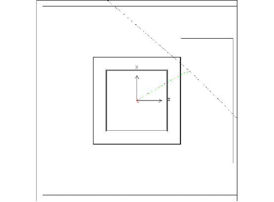
Figure 5.1: A typical $\nu n\rightarrow\mu^{-}p$ reaction in the FINeSSE detector. The event vertex is at the origin of the indicated coordinate system. In this event the $\mu^{-}$ leaves the Vertex Detector, stops in the range stack, and decays. The two neutrinos from the muon decay are seen exiting the apparatus. The short recoil proton track is just visible at the origin.

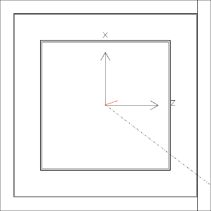
Figure 5.2: A typical $\nu p\rightarrow\nu p$ reaction expected in the FINeSSE detector, generated at the origin. The short proton track can be seen, as can the final state neutrino which exits the apparatus. In this view, only the Vertex Detector is shown.

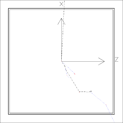
Figure 5.3: A typical $\nu n\rightarrow\nu n$ reaction expected in the FINeSSE detector. Several interactions of the final state neutron can be seen. The final state neutrino exits the apparatus. In this view, only the Vertex Detector is shown.

The individual particles within a particular event will be identified via their track length and energy loss density, “$dE/dx$”, as well as their decay patterns:

• $\mu^{\pm}$: Long tracks with low $dE/dx$. High-energy $\mu^{\pm}$ will exit the Vertex Detector and enter the veto and perhaps the range stack. For $\mu^{\pm}$ that stop in an active area, the decay (Michel) electron will be observed.

• $p$: Short tracks with high $dE/dx$. A 100 MeV proton travels approximately 10cm in liquid scintillator.

• $n$: Extraneous tracks from $\nu p$ scattering. Occasionally transfer enough energy in one collision so as to be misidentified as a $p$ track. Will thermalize and capture in the detector yielding a delayed 2.2 MeV $\gamma$.

• $\pi^{\pm}$: Longish tracks that look like $\mu^{\pm}$. For $\pi^{\pm}$ that decay in the active area of the detector, the subsequent $\mu^{\pm}$ and $e^{\pm}$ can be observed.

• $\pi^{0}$: 2 hit clusters from the $\pi^{0}$-decay $\gamma$ showers.

• $e^{\pm}$: 1 “fat” track from the $e^{\pm}$ shower.

Event Kinematics

The two-body kinematics of NC elastic ($\nu N\rightarrow\nu N$) and CCQE ($\nu n\rightarrow\mu^{-}p$) interactions are shown schematically with the use of the kinematic ellipses in Figure 5.4.

Figure 5.4: Kinematic ellipses for the NC elastic ($\nu p\rightarrow\nu N$) reaction. These are also valid for the CCQE ($\nu n\rightarrow\mu^{-}p$) reaction. The circles (ellipses) of increasing size indicate the CM (lab) momentum for the event at $E_{\nu}=$500, 1000, 1500 MeV. The longitudinal component (parallel to the beam) of the particle momentum is plotted on the x-axis, and the transverse component on the y-axis. In a particular event, the particle momentum vector is constrained to lie on the appropriate ellipse.

Due to the energy of the incident neutrino and the relatively low mass of the muon, the kinematics of the NCp and CCQE events are almost identical above $E_{\nu}\approx 300$ MeV. This simplifies the analysis and interpretation of the NC and CCQE event reconstruction. As can be seen in Figure 5.4, the final-state lepton may have any angle; the outgoing hadron has a maximum lab angle of 90^∘. The correlations can be seen in this figure as well. An event with a lower-energy high-angle lepton is paired with a low-angle high-energy hadron (and vice versa).

Plotting energy vs. angle (Fig. 5.5) reveals strong correlations between the two variables for such two-body reactions. The events of most interest for the $\Delta s$ analysis are low $Q^{2}$ events, where the proton has a low energy and a high angle. The lepton in these events will be in the forward direction at high energy. The events of most interest for the oscillation analysis are $\nu_{\mu}$ CC interactions with outgoing muons whose kinetic energy lies in the 0.1 to 1.5 GeV range. Many of these lower energy muons range out in the Vertex Detector and veto; the most energetic ones, at small angles, enter and range out in the Muon Rangestack.

The effects of Fermi momentum of the bound nucleons can be seen in Fig. 5.5, which compares the final-state protons produced in CCQE scattering from nucleons bound in carbon (Fig. 5.5b) to those from free nucleon scattering (Fig. 5.5c). Fermi momentum widens the angular distribution of the outgoing proton and suppresses the number of nucleons at low momentum (“Pauli blocking”). The effect of this additional Fermi energy ($\approx 25$MeV) on the energy of the outgoing proton is small and will have minimal impact on measuring the $Q^{2}$ of the reaction (via $Q^{2}=2m_{p}T_{p}$).

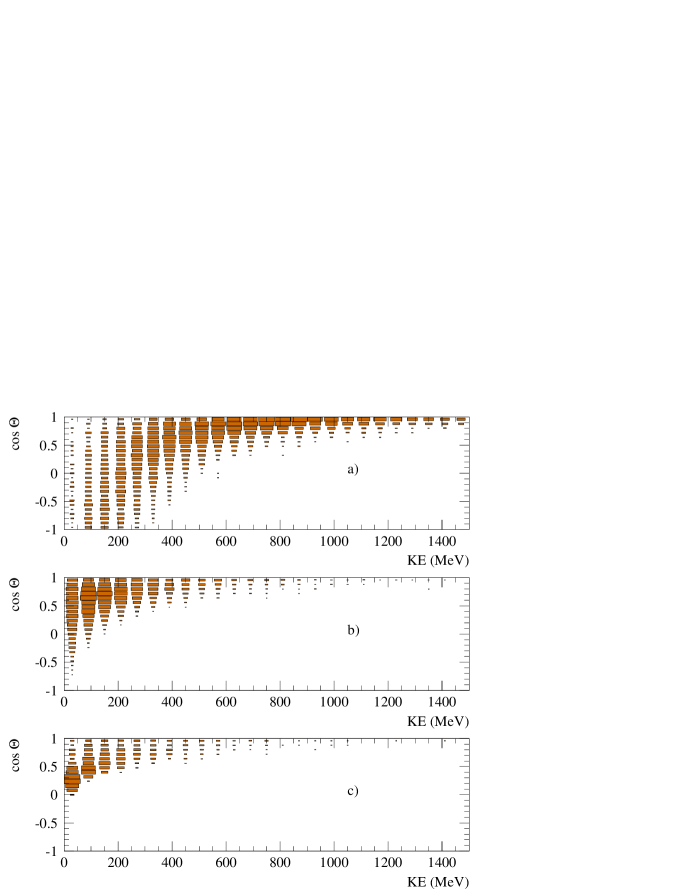
Figure 5.5: Kinetic energy vs. $\cos\theta$ for the (a) $\mu$, (b) proton in CCQE scattering from bound nucleons, and (c) proton in CCQE scattering from free nucleons. Protons in NCp reactions will show the same distribution as that in (b).

The correlations shown in Fig. 5.5 will be used to reduce backgrounds from NC and CC single pion reactions by requiring that the reconstructed tracks obey the illustrated kinematic constraints.

5.2 Simulation of the Detector

The full FINeSSE detector, including the Vertex and the Muon Rangestack subdetectors, has been simulated using the the GEANT [68] simulation package. A diagram of the apparatus as modeled by the program is shown in Fig. 5.6.

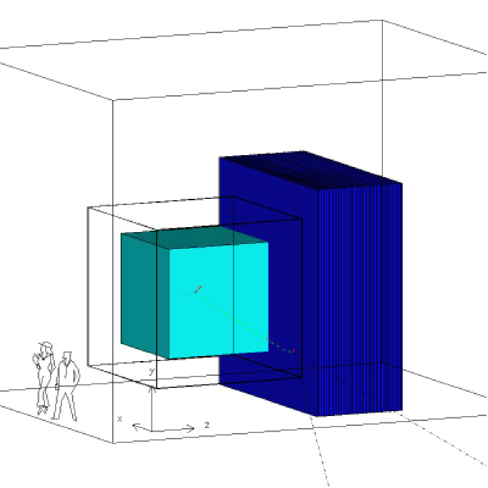
Figure 5.6: Diagram of the detector geometry as simulated by GEANT with a superimposed CCQE scattering event.

The Vertex Detector is simulated as an (2.4m)³ of liquid scintillator with a 80 $\times$ 80 grid of embedded 1.5 mm fibers with a 3.0 cm spacing in three orientations (XY, XZ, YZ; Fig. 4.3) for a total of 19,200 fibers. This inner volume containing the fibers is embedded in a larger volume of (3.5m)³ of ($\rho=0.85$ g/cm³) liquid scintillator. The fiber support structure and tank walls are also included in the simulation. The area outside of the fiber area in the scintillator tank (the “veto”) is also assumed to be active.

The Muon Rangestack, downstream of the Vertex Detector, is implemented with geometry as described in Section 4.1.2, which consists of alternating planes of scintillator and iron.

In the inner region, scintillation light and Čerenkov radiation from passing charged particles is simulated. Photons thus produced are tracked until they impinge upon a WLS fiber or the edge of the detector volume, or are absorbed. In the outer 50 cm (veto) region of the liquid scintillator and in the Muon Rangestack, individual photons are not tracked – only energy loss is recorded. However, this is not important in these regions as photostatistics are not crucial.

In the active region of liquid scintillator, it is estimated that 5000 scintillation photons are produced in the liquid scintillator for every 1 MeV of energy deposited by a charged particle [56]. The absorption and capture efficiency of photons intersecting a WLS fiber is estimated to be 5% [56]. These fibers have typical attenuation lengths of 2.5 m, and the quantum efficiency of the PMT is approximately 20%. As a result, approximately 10% of the photons emitted in the capture cone of the fiber will make it to the PMT and produce a photoelectron. Combining these two factors yields an overall efficiency of 0.5% that an optical scintillation photon that strikes a WLS fiber will be detected at the PMT. To aid the speed of the simulation, the photon detection efficiency and production was combined so that 25 ($5000\times 0.005$) photons are produced per MeV. An effective efficiency of 100% for the photons that hit a 1.5 mm WLS fiber was then assumed. In this way, the effects of photostatistics were properly simulated and the efficiency of the simulation was kept high. The attenuation length (5m) [56] of the scintillator is fairly large compared to the size of the detector and is not a significant effect. The saturation due to large localized energy deposits (“Birks’ ” Law) is also modeled. The production of Čerenkov photons is simulated but is negligible as the number of Čerenkov photons is only about 1% of that for scintillation.

Using these factors, the simulation predicts that a proton track track passing near a fiber will create on average 10 photoelectrons in the PMT. This is consistent with the prototype test results reported in Chapter 4 (factoring in the difference in fiber length). Employing this method of tracking individual optical photons in the Vertex Detector assures that the photo statistics (with fluctuations) are properly simulated.

The simulation program can track single-particle events to study the detector response for each particle type. Alternatively, it can accept event descriptions as generated by the NUANCE MC program as described in Chapter 3. The later class are events that were used to predict sensitivities as described below. The output of the detector simulation includes: a list of all the “hit” fibers in the Vertex Detector, a list of all the bars in the Muon Rangestack that recorded energy loss, and the total amount of energy and time of deposit in each area of the detector. These data are subsequently passed through the event reconstruction program.

Event Reconstruction

The simulated event data from the Vertex Detector are analyzed with a reconstruction program employing a Hough transform technique [69]. The Hough transform is a global track finding method that uses the hit fiber information from the XZ and YZ orientations. (The information from the XY orientation has not yet been used. This information can only improve the reconstruction.) The coordinates of each fiber (that recorded an amount of light over an adjustable threshold value) are used to calculate

$$R=X(Y)\sin\alpha+Z\cos\alpha~{},$$ (5.1)

where $\alpha$ is a track angle and $R$ is the perpendicular distance from the track to the origin. The track angle $\alpha$ is varied in a loop from $-90^{\circ}$ to $+90^{\circ}$, and the $R$ and $\alpha$ values for each hit used to make an entry (weighted by the amount of light in the hit) in a histogram.

The task of track finding then reduces to finding “peaks” in this histogram. Finding single tracks is quite easy with this method. For events with multiple tracks, alternate methods had to be developed and tuned to subtract the light from the first track before the algorithm was employed to find subsequent tracks. At present, the reconstruction program is limited to finding a maximum of two tracks in each of the two 2D-orientations (XZ,YZ).

The 2D-tracks were then combined to form 3D-tracks. The total energy and length of each track was also calculated, from which the $dE/dx$ of the track could be determined.

The simulated detector energy, angle, and position resolution for 50-500 MeV KE protons and muons are shown in Figure 5.7. These particle energies are representative of the tracks that will be contained in the Vertex Detector for physics events. These proton kinetic energies correspond to $Q^{2}$ values of 0.1-1.0 GeV² in NCp and CCQE reactions. A Gaussian fit to the energy and angle resolution yields $\Delta E=13(16)$ MeV and $\Delta\theta=100(80)$ mrad for protons (muons). The quantity $\Delta v$ plotted in Figure 5.7 is the distance from the calculated track origin from the true origin. The simulations of single particles predict a mean $\Delta v=9(10)$ MeV for protons (muons). The distribution is slightly wider for muons as they are longer tracks. These results indicate detector performance that will meet the physics goals of the experiment. The effect of detector resolution on the physics distributions will be shown in the following sections.

Comparison with IU Cyclotron Facility Prototype Tests

The results of these resolution studies are consistent with the prototype tests performed at the IUCF (described in Chapter 4), factoring in the differences in the two studies. For example, the prototype detector was much smaller (and so did not fully contain tracks); had only one fiber orientation; and used a slightly different fiber spacing. Nevertheless, the tracks reconstructed from the prototype test data yielded an angular resolution of approximately 6^∘ (15^∘ FWHM). The resolution quoted in Section 5.2 for protons is also 6^∘. Similarly, the amount of light detected in the IUCF tests was $17\pm 2$ photoelectrons for a 200 MeV passing adjacent to a fiber. These simulations, with light collection and detection efficiencies estimated from the individual detector properties, are in agreement with these results.

Figure 5.7: The energy (a,b), angle (c,d), and position (e,f) resolution of the Vertex Detector as simulated and reconstructed for a sample of 1000 single particle events. The plots on the left (a,c,e) are for 50-500 MeV KE protons, those on the right (b,d,f) for 50-500 MeV KE muons. Only tracks that were fully contained in the Vertex Detector were selected. This effectively limited the upper muon KE to $\approx 300$ MeV.

5.2.1 Events in the Vertex Detector

Several examples of the tracks obtained with the Hough transform reconstruction method from simulated data are shown in Figures 5.8 and 5.9. In these figures, the particle directions are indicated by the light-colored arrows. The reconstructed tracks and endpoints are indicated by dark lines and dots. As indicated, this method results in accurate reconstructed tracks for muons and protons down to kinetic energies of 100 MeV.

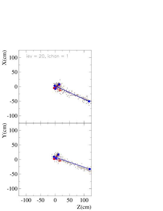
Figure 5.8: A XZ (top) and YZ (bottom) projection view of a CCQE event in the simulated Vertex Detector with the reconstructed muon (long line) and proton (short line) tracks superimposed. In this event, $T_{\mu}=820$ MeV and $T_{p}=150$ MeV.

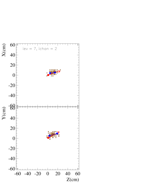
Figure 5.9: A XZ (top) and YZ (bottom) projection view of a NCp event in the simulated Vertex Detector with the reconstructed proton track superimposed. In this event, $T_{p}=100$ MeV.

5.2.2 Events in the Muon Rangestack

Events in the Muon Rangestack considered here, have reconstructed vertices in the Vertex Detector fiducial volume, exit the Vertex Detector, and enter the Rangestack. These higher energy muons tend to be emitted at small angles as indicated by Figure 5.5a, which shows the outgoing angle of the muon as a function of the muon energy. The energy distribution of these muons events that enter and stop in the Muon Rangestack is shown in figure 5.10, superimposed over the distribution for all muons. The distribution of hits as a function of transverse position in the range stack created by these higher energy muons is shown in Figure 5.11. Note that there are few hits near edges of the Rangestack. A muon is considered to have ranged out in this subdetector if its last hit is not at an edge of the detector, either in the last plane, or one of the edge strips of an earlier plane for higher angle muons. Most muons below 1.5 GeV range out within the Rangestack as indicated by hits deposited in each rangeout layer (Figure 5.12).

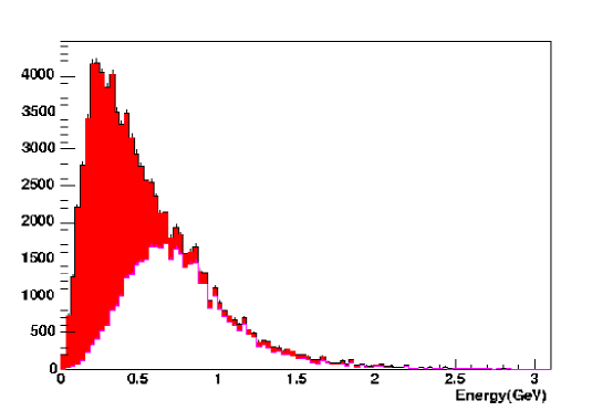
Figure 5.10: The energy distribution of muons from CCQE interactions within the Vertex Detector fiducial volume, that enter and range out in the Muon Rangestack(white) overlaid on the distribution of all muons(red).

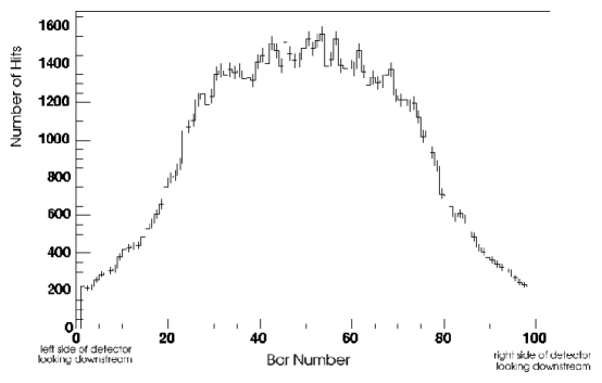
Figure 5.11: Number of hits in scintillator strips in the Muon Rangestack from CCQE muons that originate in the Vertex Detector fiducial volume. The “Bar Number” measures the hit coordinate transverse to the beam direction.

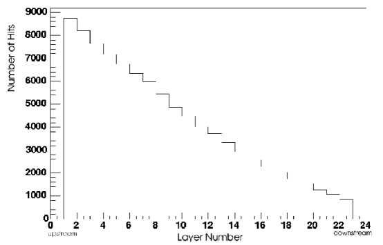
Figure 5.12: Number of hits in each scintillator layer in the Muon Rangestack from CCQE muons that originate in the Vertex Detector fiducial volume. The “Layer Number” measures the coordinate along the beam direction.

5.3 Backgrounds

We recognize two major classifications of backgrounds for FINeSSE: beam related and beam unrelated.

FINeSSE can expect to see background events from neutrino interactions in the detector through channels other than $\nu_{\mu}$ CC and NC events, as described in Section 3.2. Some of these will be misidentified as signal channel interactions. There will also be neutrino interactions in the dirt around the detector, sending charged particles and neutrons into the detector. These are the most important beam related backgrounds.

FINeSSE will also see a large flux of cosmic ray muons and neutrons. These events can be used for detector calibration, as described in Section 4.1.4, but they can also be misidentified as beam events and therefore represent a potential background. However, the small probability of an interaction in time with the short beam spill of the booster neutrino source (1.6 $\mu$s) reduces these backgrounds greatly. In addition, they can be accurately measured and subtracted.

5.3.1 Beam Related Backgrounds

The NC and CC measurements will have very different backgrounds, due to differences in their event topologies. The CC events have an outgoing muon and a recoil proton. These two particles emitted from the interaction vertex will usually provide a very clean signal. However, at low $Q^{2}$, where $\Delta s$ is measured, the recoil proton will have very little energy. In these cases, charged particles from other interactions with two final states could mimic this short, proton-like track. The NC events have only the recoil proton. Interactions producing only low energy short tracks can mimic this recoil proton. These will be the hardest events to identify.

Tables 3.1 and 5.3 list the expected event rates from the neutrino beam. FINeSSE expects to see 24,435 CCQE events and 9864 NC elastic events per $1\times 10^{20}$ POT, assuming 100% detection and reconstruction efficiencies. Using the present selection cuts, the expected event totals are 2990 CCQE events and 1604 NC elastic signal events per $1\times 10^{20}$ POT. Because the $\Delta s$ analysis will use a ratio to eliminate many systematic uncertainties, background events become a significant challenge to the measurement. Table 5.3 summarizes the contributions to the signal from beam related backgrounds that originate in the detector.

Neutrons from beam neutrino interactions in the material around the detector are an additional potential background. These events arise from neutrino NC and CC interactions in the material around the detector that create secondary particles that impinge on and interact in the detector. The majority of the events cannot be eliminated by taking advantage of the Booster neutrino beamline timing structure, as they will be in time with the beam. The majority of the particles that mimic a signal are neutrons that are produced in the surrounding dirt. They have a fairly large range and can travel into the central area of the detector without leaving a signal in the edge. Muons, can not do this and, therefore, are not a background.

Initial Monte Carlo studies, employing the cuts described in Section 5.3.4, indicate that the number of neutrons that interact in the dirt around FINeSSE and pass the particle ID cuts are insignificant compared to the signal.

An additional background to consider are neutrons directly produced by protons in the booster neutrino source beam dump. These neutrons will constitute a negligible background at the FINeSSE detector enclosure 50m downstream from the dump. There is no significant neutron flux from the beam dump after 25m downstream due to absorption in the earth. This was determined in shielding assessment studies for the Booster neutrino source [70].

5.3.2 Beam Unrelated Backgrounds

The main beam unrelated backgrounds stem from cosmic rays. After selection cuts, these are negligible in comparison with the NC elastic signal. The cosmic ray muon rate in the FINeSSE detector fiducial volume, beneath 1 m of concrete and 0.5 m of veto region scintillator, will be about 900 Hz. The muons are a potential background both for CC and for NC events. The relative rate of coincidences with the beam timing window is 0.0014. This can be reduced to $1.4\times 10^{-6}$ by factoring in a conservative veto efficiency of 0.999 for muons. At 0.5 m thick, the veto for the Vertex Detector will be more efficient than the 0.3 m thick MiniBooNE veto, which has an efficiency better than 1 in $10^{4}$ for through-going muons.

Unlike the beam related backgrounds, the number of background events considered here depends on the Booster performance. If we assume that the Booster delivers $4\times 10^{12}$ protons per pulse, then we expect to see 36 non-vetoed cosmic ray muon events per $1\times 10^{20}$ POT in coincidence with the beam. Event analysis will reduce this background down further; since there will be no recoil proton and the muons will all be headed downward. Therefore, cosmic ray muons will present a negligible background to CCQE or NC events.

Cosmic ray neutrons have also been considered as a background. Their average rate above 50 MeV during periods of normal solar activity at sea level and $\sim 40^{\circ}$ geomagnetic latitude is approximately $9\times 10^{-3}$sec^-1cm^-2 [71, 72]. They have a momentum spectrum that falls very steeply with energy. Fewer than 5% of these can traverse the concrete shielding and the veto region. We therefore expect a cosmic neutron rate of $<1$Hz in the FINeSSE Vertex Detector, for neutrons above 100 MeV. This rate will be reduced to a negligible level because of the small coincidence probability with the short beam spill.

5.3.3 Charged and Neutral Current Event Identification

Neutral-current elastic scattering events ($\nu p\rightarrow\nu p$) will be identified in the FINeSSE detector by looking for single proton tracks consistent with elastic scattering kinematics. A track is identified as a proton by a large $dE/dx$. Charged-current quasi-elastic scattering events ($\nu n\rightarrow\mu^{-}p$) will be identified by looking for events with two tracks each consistent with the expected $dE/dx$. In addition, other cuts are employed to reject backgrounds. The strategy will be to maintain a compromise between large efficiency for low-$Q^{2}$ events while keeping backgrounds as low as possible. The squared four-momentum transfer, $Q^{2}$, will be determined event by event, by measuring the energy of the proton in both NC and CC events. $Q^{2}$ is determined from the energy via $Q^{2}=2m_{p}T_{p}$.

5.3.4 Simulation Results

The GEANT simulation of the FINeSSE detector and reconstruction program as described above is used to estimate efficiencies and backgrounds for the NC/CC ratio measurement. It is also relied upon to determine the experimental error on a measurement of $G_{A}^{s}$.

Cuts

The experimental cuts employed for $\nu p\rightarrow\nu p$ (NCp) and $\nu n\rightarrow\mu^{-}p$ (CCQE) event identification are summarized in Table 5.2. A reasonable compromise of efficiency and background rejection could be obtained out to within 15 cm of the edge of the active Vertex Detector volume. This results in a fiducial volume of (2.2 m)³ = 10.6m³ or 68.4% of the total (2.4 m)³ “active” volume of the Vertex Detector. With $\rho=0.85$ g/cm³ liquid scintillator, a fiducial mass of 9.1 t is obtained.

cut #	NCp cuts	CCQE cuts
0	edge distance $<$ 15cm	edge distance $<$ 15cm
1	# 3d tracks = 1	# 3d tracks.eq.2
2	$dE/dx(p)>2.5$	$dE/dx(p)>2.5,dE/dx(\mu)<2.5$
3	$\theta(p)>0.5$	$\theta(p)+\theta(\mu)>1.5$
4	no “late” light in vertex det.	no “late” light in vertex det.
5	no veto or muon stack energy	low “remaining” energy

Table 5.2: Cuts used to identify “NCp” and “CCQE” events in the simulated sample.

Cuts 1 and 2 identify and separate NCp and CCQE based on the number and type of charged particle tracks in the event. Cut 2 accepts events with tracks of larger angle, a feature of the two-body kinematics of these events, and rejects background events which tend to have tracks at smaller angles. Cut 4 lowers background by eliminating pions that stop and decay in the Vertex Detector into muons (which decay “late”). This also has a slight effect on the efficiency for accepting CCQE events, but it is not large since most of the muons in CCQE scattering leave the Vertex Detector. Cut 5 lowers backgrounds for both channels. For NCp events, it further lowers the pion (charged and neutral) backgrounds by cutting those events where the pions leave little signal in the Vertex Detector. For CCQE, events cut 5 also reduced pion backgrounds as a cut on low “remaining” energy (energy not assigned to tracks after tracking is complete) reduces the number of events with extra energy (due to pions).

Efficiencies and Purities

A sample of 215k NUANCE-generated events were tracked through the detector with the GEANT simulation with vertices evenly distributed within the nominal volume of the Vertex Detector (2.4 m)³. These events are then reconstructed using the algorithms described above. The results are summarized in Table 5.3.

	reaction channel
NCp cuts	NCp	NCn	NC$\pi$	CCQE	CC$\pi$
raw events	21219	20487	19062	100102	54107
passed events	3929	1162	167	48	4
efficiency (%)	18.5	5.7	0.9	0.0	0.0
fid. eff. (%)	27.1	8.3	1.3	0.1	0.0
purity (%)	74.0	21.9	3.1	0.9	0.1
CCQE cuts	NCp	NCn	NC$\pi$	CCQE	CC$\pi$
raw events	21219	20487	19062	100102	54107
passed events	165	76	581	7323	1322
efficiency (%)	0.8	0.4	3.0	7.3	2.4
fid. eff. (%)	1.1	0.5	4.5	10.6	3.6
purity (%)	1.7	0.8	6.1	77.4	14.0

Table 5.3: Summary of events that passed the NCp and CCQE cuts along with efficiencies and purities: “efficiency” is the reconstruction efficiency throughout the (2.4 m)³ volume. “fid. eff.” is the reconstruction efficiency within the (2.2 m)³ fiducial volume. The simulation data set contained 215k events. To scale to the total expected FINeSSE event count, multiply these numbers by 2.45.

The efficiencies and $Q^{2}$ resolutions for the NCp and CCQE “signal” samples are shown in Figures 5.13 and 5.14. Note the large efficiency for reconstructing NCp, and reasonable efficiency for CCQE, in the $Q^{2}=0.2-0.4$ GeV² region. At low $Q^{2}$, proton tracks from NCp are short and difficult to reconstruct, causing a fall off in the efficiency. At high $Q^{2}$, final state particles tend not to be contained for both the NCp and CCQE samples, causing a fall of in the efficiency in these regions also. In addition to this, very forward events in the NCp sample are cut to remove backgrounds from pions. This further decreases the NCp efficiency at high $Q^{2}$.

Figure 5.13: (a) Efficiency for reconstructing true NCp events with the NCp cuts within the fiducial volume as a function of generated $Q^{2}$ and (b) the distribution of the difference between generated and reconstructed $Q^{2}$ for this sample. The $\sigma$ of this distribution is 0.053 GeV²

Figure 5.14: (a) Efficiency for reconstructing true CCQE events with the CCQE cuts within the fiducial volume as a function of generated $Q^{2}$ and (b) the distribution of the difference between generated and reconstructed $Q^{2}$ for this sample. The $\sigma$ of this distribution is 0.079 GeV²

5.3.5 Method to Extract $\Delta s$ from the Data

To extract $\Delta s$ (or $G_{A}^{s}$) from the data, the NC to CC ratio must be formed and compared to predictions obtained from Eq. 2.5. This ratio must be corrected for backgrounds and detector efficiency and may be written as:

$$R(NC/CC)=\frac{\epsilon_{\mathrm{CC}}}{\epsilon_{\mathrm{NC}}}\frac{(N_{\mathrm{NC}}-\sum_{i}\epsilon_{\mathrm{NC},i}N_{\mathrm{NC},i})}{(N_{\mathrm{CC}}-\sum_{j}\epsilon_{\mathrm{CC},j}N_{\mathrm{CC},j})}~{},$$ (5.2)

where $\epsilon_{\mathrm{NC}}$ ($\epsilon_{\mathrm{CC}}$) is the NC (CC) reconstruction efficiency, and $N_{\mathrm{NC}}$ ($N_{\mathrm{CC}}$) is the number of NC (CC) identified events in the detector. The quantities $\epsilon_{\mathrm{NC},i},\epsilon_{\mathrm{CC},i},N_{\mathrm{NC},i},$ and $N_{\mathrm{CC},i}$ are the background efficiencies and calculated number of background events for the NC and CC channels, respectively.

Each of the terms in Equation 5.2 will contribute to the total error on $R(NC/CC)$. The relationship between the error on $G_{A}^{s}$ ($\sigma(G_{A}^{s})$) and R is quantified in Eq. 2.13, so we can estimate the error on $G_{A}^{s}$ due to each of the terms in Eq. 5.2. These errors are discussed and quantified in the sections below, assuming that the measurement is performed in the $Q^{2}=0.2-0.4$ GeV² bin, and that an estimate of $\sigma(G_{A}^{s})$ is obtained. After this treatment, a fitting procedure that uses the entire range of $Q^{2}$ is used, to illustrate an improved method for extracting $G_{A}^{s}$.

Statistical Errors

The event sample of 215k NUANCE-generated events is 0.408 of the total number of neutrino-scattering events expected in the (2.4 m)³ active volume of the Vertex Detector with $6\times 10^{20}$ POT. So the number of events in Table 5.3 may be multiplied by $1/0.408=2.45$ to obtain the total number expected. Taking these scaled numbers, and considering the efficiencies for the NCp and CCQE cuts, yields 7341 (9936) accepted events in the NCp (CCQE) sample in the $Q^{2}=0.2-0.4$ GeV² bin. Statistical errors from these two sources will contribute 1.2% and 1.0% to the relative error on R(NC/CC).

Neutral Current Neutrino Neutron Scattering

One of the backgrounds in the numerator of Equation 5.2 is that due to the NC process $\nu n\rightarrow\nu n$ (labeled “NCn” in Table 5.3). This reaction will need to be treated separately, since it is the largest background to the NCp channel, and also since the rate depends upon $G_{A}^{s}$.

The dependence of cross section for $\nu n\rightarrow\nu n$ on $G_{A}^{s}$ is different than that for $\nu p\rightarrow\nu p$, due to the isospin factor $\tau_{z}$ (cf. Equation 2.9). This will “dilute” the experimental sensitivity. For this reason it is important to keep the efficiency of the $\nu n\rightarrow\nu n$ channel as low as possible. This is a difficult task as neutrons in a liquid scintillator detector often undergo charge-exchange reactions which create energetic protons. These reactions can be indistinguishable from the $\nu p\rightarrow\nu p$ reaction. Neutrons, though, often create two or more protons of lower energy and these topologies will not be misidentified as $\nu p\rightarrow\nu p$.

As can be seen from Table 5.3, the reconstruction efficiency for the NCn background is 8.3% and comprises 21.9% of the NCp sample. It is non-negligible. It would be desirable to improve the detector and reconstruction to lower this background. It is likely that this is possible by observing the delayed light due to neutron capture. The detector as currently designed would have the ability to observe this delayed light, and this would improve the neutron background rejection considerably. This technique, however, has yet to be investigated fully, and any potential gains are not assumed in this analysis.

The effect of NCn events in the NCp sample dilutes the sensitivity of the measured NC to CC ratio to $G_{A}^{s}$ by a factor $(1-2\epsilon_{\mathrm{NCn}}/\epsilon_{\mathrm{NCp}})$. The impact of this on the analysis can be determined using the ratio of efficiencies, $\epsilon_{\mathrm{NCn}}/\epsilon_{\mathrm{NCp}}$ = 0.19, in the $Q^{2}=0.2-0.4$ GeV² bin. Applying this efficiency factor, the sensitivity of R(NC/CC) is reduced from 1.2 to 0.75. This is a fairly substantial reduction but not large enough to prevent a measurement. The uncertainty in $G_{A}^{s}$ becomes:

$$\sigma(G_{A}^{s})=1.3\Delta R/R.$$ (5.3)

A 5% relative measurement of the NC/CC ratio at $Q^{2}=0.25$ GeV² would enable an extraction of $G_{A}^{s}$ with an error of 0.07.

Scattering from Free Protons

The FINeSSE neutrino scattering target is mineral-oil-based liquid scintillator (mainly CH₂). The hydrogen will provide two additional free protons for $\nu p\rightarrow\nu p$ scattering. This entails a correction to the measured NC to CC ratio. The measured ratio (after background subtraction) will be:

$$\frac{N_{\mathrm{NC}}}{N_{\mathrm{CC}}}=\frac{N_{\mathrm{NC}}^{\mathrm{C}}+N_{\mathrm{NC}}^{\mathrm{free}}}{N_{\mathrm{CC}}}~{},$$ (5.4)

where $N_{\mathrm{NC}}^{\mathrm{C}}$ and $N_{\mathrm{NC}}^{\mathrm{free}}$ are the number of events from $\nu p\rightarrow\nu p$ on bound (in carbon) and free protons. This can be written:

$$\frac{N_{\mathrm{NC}}}{N_{\mathrm{CC}}}=\frac{N_{\mathrm{NC}}^{\mathrm{C}}}{N_{\mathrm{CC}}}\times(1+\mathcal{F})~{},$$ (5.5)

where:

$$\mathcal{F}=\frac{N_{\mathrm{NC}}^{\mathrm{free}}}{N_{\mathrm{NC}}^{\mathrm{C}}}.$$ (5.6)

Naively, one would expect $\mathcal{F}$ to be equal to the free proton to bound ratio in the target. This is $\approx 0.34$ [73] for mineral-oil-based liquid scintillator. In actuality, $\mathcal{F}$ will be slightly larger than these numbers, as the the cross section per nucleon is slightly suppressed (by $\approx 10\%$) for bound nucleons. In addition, the value used for $\mathcal{F}$ will depend upon the $Q^{2}$ region accepted for the analysis. So for the purposes of a conservative estimate here, $\mathcal{F}=0.34*1.10=0.38$ will be used.

The desired corrected ratio (that on pure carbon) can then be written:

$$R(NC/CC)=\frac{N_{\mathrm{NC}}^{\mathrm{C}}}{N_{\mathrm{CC}}}=\frac{1}{(1+\mathcal{F})}\frac{N_{\mathrm{NC}}}{N_{\mathrm{CC}}}~{};{\mathrm{and}}$$ (5.7)

$$\frac{\Delta R}{R}=\frac{\mathcal{F}}{1+\mathcal{F}}\frac{\Delta\mathcal{F}}{\mathcal{F}}=0.27\frac{\Delta\mathcal{F}}{\mathcal{F}}~{}.$$ (5.8)

The number of bound and free protons in the target will be known, so the relative uncertainty on $\mathcal{F}$ will be dominated by the uncertainty in the ratio of the bound to free NC cross sections. An estimate of this relative uncertainty is 5%. This will add a systematic uncertainty in the NC to CC ratio of $\approx 1.4\%$.

Systematic Error in Efficiencies

The flux and target density is same for both NC and CC reactions and does not enter as an additional source of uncertainty in a measurement of the ratio, R(NC/CC). However the reconstruction efficiencies will not be the same for both reactions, and the systematic error in the $\frac{\epsilon_{\mathrm{CC}}}{\epsilon_{\mathrm{NC}}}$ term of Eq. 5.2 must be considered.

At a given $Q^{2}$, the proton in the NC and CC reactions has the same kinematics. Because of this, some of the systematic error is highly correlated and the dominant uncertainty is in the efficiency to detect the muon in the CC reaction. This is a well-understood process and it should be possible to determine it with high accuracy. For these reasons, a relative error of 3% is estimated for $\frac{\epsilon_{\mathrm{CC}}}{\epsilon_{\mathrm{NC}}}$ and will contribute at this level to the relative error on R(NC/CC).

Systematic Error in Backgrounds

The background subtraction in both the numerator and denominator of Equation 5.2 also contributes systematic error to R(NC/CC). This error has a contribution from both the absolute rate of the background and the efficiency to be reconstructed as a NCp or CCQE event. The relative error on R(NC/CC) due to these uncertainties is diluted to the reasonably small background subtraction. This dilution factor is equal to the ratio of background to (true) signal for NCp and CCQE events. From the numbers in Table 5.3 this dilution factor is 0.35 for NC events and 0.29 for CC events.

It is estimated that the relative error on the product of efficiency times background can be kept at or below 10% for both NC and CC reactions. This will be possible by means of detailed simulations and studies of the detector, and having developed a good model for the background processes. These backgrounds have been measured in other neutrino experiments, and likewise, will be measured in FINeSSE. In addition, relevant electron scattering data exist.

The relative error of 10% on the background contributions contributes 3.5% (2.9%) via NC (CC) backgrounds to the relative error on R(NC/CC).

Systematic Error Due to $Q^{2}$ Reconstruction

A large error in the $Q^{2}$ reconstruction of events will distort the overall distribution and add to the error in R(NC/CC). For example, if low-$Q^{2}$ ($<0.2$ GeV²) CCQE events (of which there are many; see Figure 2.3) are reconstructed in the $Q^{2}=0.2-0.4$ GeV² bin, a larger error will result in R(NC/CC) that is not quantified in the errors considered above.

From examination of Figures 5.13 and 5.14, it can be seen that the $Q^{2}$ resolution of this detector is quite good for both NCp and NCn events. Also, there is no evidence of a large skew in these distributions. The $Q^{2}$ resolution is smaller than the bin width and will contribute a negligible error to R(NC/CC).

This hypothesis is further checked in the fitting procedure described below as the reconstructed $Q^{2}$ is used to bin the data.

Nuclear Model Uncertainties

The majority of protons and neutrons participating in $\nu p\rightarrow\nu p$ and $\nu n\rightarrow\mu^{-}p$ interactions are not free, but are bound within a carbon nucleus. Any nuclear effects that are not symmetric between protons and neutrons can lead to a misinterpretation of the data, when analyzed using a free nucleon model. For this reason, a model with a realistic treatment of nuclear effects will be employed for the final analysis.

The sensitivity of the NC and CC cross sections to the specific nuclear model employed has been investigated by several different groups [27, 32, 33]. The effects on the absolute cross sections can be quite dramatic. However, the distortion in the ratio R(NC/CC) has been shown to be small. It has been estimated to introduce an error on 0.005 in $G_{A}^{s}$ [34].

This will be an area of continuing work. Results up to now, however, indicate that R(NC/CC) is insensitive to the details of the nuclear model employed for the calculations.

Form Factor Uncertainties

The (non-strange) form factors in Eq. 2.5 have been measured in a variety of experiments at many different $Q^{2}$ values. This is not true for the strange form factors. Information on the strange-axial form factor $G_{A}^{s}$ is almost completely non-existent. Accumulating more information on this form factor is one of the main goals of this experiment. The strange vector form factors influence the NC to CC ratio only weakly and they will be precisely measured by the upcoming G0 experiment [16] to take place a Jefferson Lab in the near future.

In addition, the contribution from these unknown form factors is minimized by performing these measurements at low-$Q^{2}$. The sensitivity of the final result to these other form factors is small as will be shown in the results from the fitting procedure below.

Summary of Errors on R(NC/CC)

The experimental systematic errors discussed in the proceeding sections are summarized in Table 5.4. These contributions, added in quadrature, yields a relative error on the ratio, R(NC/CC), of 5.8%. This, combined with Equation 5.3, yields a total error on $G_{A}^{s}$ of 0.075.

quantity,		relative error,	contribution to
$Q$	prefactor	$\Delta Q/Q$	$\Delta R/R$
$N_{\mathrm{NC}}$	1	1.2%	1.2%
$N_{\mathrm{CC}}$	1	1.0%	1.0%
$\mathcal{F}=\frac{N_{\mathrm{NC}}^{\mathrm{free}}}{N_{\mathrm{NC}}^{\mathrm{C}}}$	0.27	5%	1.4%
$\frac{\epsilon_{\mathrm{CC}}}{\epsilon_{\mathrm{NC}}}$	1	3%	3.0%
$\sum_{i}\epsilon_{\mathrm{NC},i}N_{\mathrm{NC},i}$	0.35	10%	3.5%
$\sum_{i}\epsilon_{\mathrm{CC},i}N_{\mathrm{CC},i}$	0.29	10%	2.9%
Total experimental error			5.8%

Table 5.4: Estimated experimental errors on a measurement of R(NC/CC) at $Q^{2}=0.2-0.4$ GeV² with FINeSSE. The prefactor relates the relative error on the quantity to the relative error on R(NC/CC). The details are explained in the text.

This is a conservative estimate. This error will be reduced considerably by reducing the $\nu n\rightarrow\nu n$ background (via detection of photons from neutron capture), which both contributes to the error in R(NC/CC) and lowers the sensitivity of $G_{A}^{s}$ to R(NC/CC).

5.3.6 A Fit Procedure to Extract $\Delta s$ from R(NC/CC)

In the error analysis explained above, only one $Q^{2}$ bin was considered. This yielded a conservative estimate for the error on $G_{A}^{s}$. As can be seen in Figures 5.13 and 5.14, high reconstruction efficiency is obtained from $Q^{2}=0.2$ to 0.8 GeV², and a measurement of R(NC/CC) may be made in this range. This larger $Q^{2}$ range will accept more events and will allow for the systematic study of the behavior of R(NC/CC) and, consequently, the form factors as a function of $Q^{2}$.

To utilize the entire data set, a fit procedure was developed to extract $G_{A}^{s}$, to determine the effects of systematic errors, and to investigate the dependence of the extracted $G_{A}^{s}$ on the other form factors. In this procedure, a corrected NC to CC ratio is formed using Equation 5.2 for each $Q^{2}$ bin of width 0.1 GeV² using the simulated data. The backgrounds are subtracted and efficiency corrections are applied. The predicted ratio is then calculated using the free nucleon cross section (Eq. 2.5), correcting for the NC scattering from free protons and the estimated contribution from $\nu n\rightarrow\nu n$. This prediction is calculated for a range of $G_{A}^{s}$ values. The dependence on the other form factors ($F_{1}^{s}$, $F_{2}^{2}$) and the axial mass $M_{A}$ is also studied.

The sensitivity of the data to $G_{A}^{s}$ is determined by calculating:

$$\chi^{2}=\sum_{i}\frac{(R_{\mathrm{meas}}-R_{\mathrm{pred}})^{2}}{\sigma(R)^{2}}~{},$$ (5.9)

where the sum runs over $Q^{2}$ bins. The $1\sigma$ error on $G_{A}^{s}$ is determined by the $G_{A}^{s}$ value where the $\chi^{2}$ value changes by 1.

This procedure yields an error on $G_{A}^{s}$ of 0.039. This is considerably smaller than the error quoted above due to the fact that this fit procedure uses more of the data through a range in $Q^{2}$.

The sensitivity of R(NC/CC) to other form factors is also studied with this method. Figure 5.15 shows how a measurement of R(NC/CC) depends on other form factors. An uncertainty in the axial vector mass, $M_{A}$, which parameterizes the $Q^{2}$ evolution of the $G_{1}$ form factor, effectively adds a small additional uncertainty to the extracted value of $G_{A}^{s}$. The current world average of $M_{A}$ as measured in neutrino scattering is $1.026\pm 0.021$ GeV [28]. This uncertainty will add approximately 0.015 to the uncertainty in $G_{A}^{s}$. The sensitivity of $G_{A}^{s}$ on $F_{2}^{s}$ is weaker, but this form factor is not well known directly. Linear combinations of this form factor with $F_{1}^{s}$ have been measured [13]. A conservative estimate on the uncertainty on $F_{2}^{s}$ is $\pm 0.1$. An uncertainty of this size in $F_{2}^{s}$ will contribute an uncertainty of $\pm 0.02$ to $G_{A}^{s}$. Combining these yields a $\pm 0.025$ uncertainty on $G_{A}^{s}$.

Figure 5.15: $\chi^{2}$ contours corresponding to $1\sigma$ (solid), $2\sigma$ (dashed), and $3\sigma$ (dotted) resulting from the fit procedure described in the text. In (a) $G_{A}^{s}$ and $M_{A}$, the axial vector mass, are varied, in (b) $G_{A}^{s}$ and $F_{2}^{s}$ are varied.

Based on the studies described above, FINeSSE will be capable of a measurement of $G_{A}^{s}$ with small errors. An uncertainty of approximately 0.04 results from considering statistical and systematic experimental errors. Uncertainties in the form factors adds an additional contribution of 0.025. This level of accuracy is unprecedented in $\nu$ scattering will allow for stringent tests with theory.

5.4 Details of $\nu_{\mu}$ Disappearance Sensitivity Studies

The method for determining the $\nu_{\mu}$ disappearance sensitivity compares the energy distribution of events in the near (FINeSSE) and far (MiniBooNE) detector. In this section we justify the choice of the experimental setup and the estimates of the systematic errors. We studied various configurations for FINeSSE+MiniBooNE running in order to identify the optimal experimental set-up. Here, we reduce the comparisons to two representative positions of the near detector (100 m and 200 m) and the two possible lengths of the decay region (25 m and 50 m). The event rates assumed in these studies are indicated in Table 5.5.

Events for $6\times 10^{20}$ POT
Location	25 m Absorber	50 m Absorber
100 m (9 t)	103,000	195,000
200 m (40 t)	97,000	162,000
550 m (650 t)	205,000	323,000

Table 5.5: Estimated event sample for $5\times 10^{20}$ POT with detectors located at various distances with fiducial volumes as given. Rates are given for a 25 m and 50 m absorber.

5.4.1 Tools and Assumptions for This Study

Determination of the $\nu_{\mu}$ disappearance sensitivity requires tools from both FINeSSE and MiniBooNE. Assumptions related to the flux in both detector have been described in Chapter 3. As discussed there, the NUANCE Monte Carlo was used to simulate events in both detectors [54]. The following standard MiniBooNE detector cuts were used: tank hits $>$ 100, veto hits $<$ 6, and reconstructed fiducial radius $<$ 500 cm.[4].

FINeSSE and MiniBooNE are assumed to have the same reconstruction efficiency. This is conservative because the finely segmented FINeSSE detector will have much better resolution on the reconstructed neutrino energy in quasi-elastic (QE) events. Energy resolution for muons ranging out in the Muon Rangestack will also be known to 10% (see Section 4.1.2). FINeSSE will also have much higher purity for the QE sample due to its excellent low energy reconstruction. For events to be counted in the FINeSSE data sample for this analysis, outgoing muons from $\nu_{\mu}$ CC interactions must be contained entirely in the Vertex Detector, in the Vertex Detector plus the veto, or in these plus the Muon Rangestack. Contributions from these three contained samples, as a function of energy, are shown in Figure 5.16. Wiggles in this distribution, seen clearly in Figure 5.17, are due to contributions from one distribution turning off as another turns on. Folding this acceptance into overall number of interactions expected yield the event rates summarized in Table 5.5.

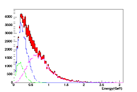
Figure 5.16: True kinetic energy distribution for all muons from CCQE interactions in the Vertex Detector fiducial volume shown in red. Overlaid in white is the sample of those with a contained muon. Also shown are contributions corresponding to muons stopping in the Vertex Detector (green), the Vertex Detector veto (blue), and the Muon Rangestack (purple).

Figure 5.17: Acceptance versus true kinetic energy for muons from the CCQE event sample.

5.4.2 The Motivation for 25 m Absorber Running: Parallax

Figure 5.18: Left, solid: Angular acceptance of the FINeSSE detector with the 50 m absorber in radians; Right, solid: Acceptance with the 25 m absorber in radians. Dashed (both plots): acceptance of the MiniBooNE detector in radians.

Figure 5.19: Left: Ratio of the $\nu_{\mu}$ flux in the FINeSSE to the MiniBooNE detector using the 50 m absorber; right: Ratio when 25m absorber is installed

The main physics driver for the FINeSSE+MiniBooNE standard configuration was reduction of “parallax” in the near detector. In this section, we describe the cause of parallax, why it is a significant issue for disappearance experiments, and how we have mitigated the effect with our design.

In an ideal world, there are two reasons why disappearance experiments based on near/far detector comparisons would be performed with point-source beams. First, the $L$ of each detector is well determined. Second, the near and far detector have the same energy and angular acceptance for the neutrinos. Unfortunately, the only true point sources come from beams created by stopped pion and muon decay (for example at LANL or SNS). These neutrinos are so low in energy that a muon cannot be produced in CC interactions. Hence $\nu_{\mu}$ disappearance searches are impossible.

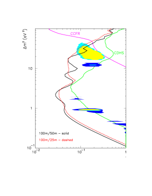
Figure 5.20: Comparison of the parameter space covered by FINeSSE+MiniBooNE with the 25 m absorber (red) and the 50 m absorber (black). The unwanted “wiggles” in the 50 m absorber allowed region are caused by the variations in the ratio of fluxes at FINeSSE and MiniBooNE.

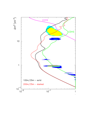
Figure 5.21: Comparison of the parameter space covered by FINeSSE+MiniBooNE for a detector at 100 m (black) from the target versus 200 m (red) from the target. Sensitivity to high $\Delta m^{2}$ is lost at 200 m because neutrinos will oscillate before reaching the FINeSSE detector.

To produce a higher energy neutrino beam, an extended decay path is necessary. In this case, the modification of $L$ for the decay length must be taken into account. Also, the angular acceptance of the detector will vary depending on the point along the line of the decay. For a detector which is relatively far from the beamline, such as is the case with MiniBooNE, these corrections are negligible. But for a near detector, this “parallax” can be a large effect.

Because there is a strong correlation between energy and angle of the neutrinos, differences in angular acceptance between the near and far detectors is a major concern. These differences translate directly into differences in the energy distribution of events. When taking a near/far ratio, the result are “wiggles,” which are not related to oscillations. As long as those wiggles do not mimic an oscillation signal, this is not a major problem. But with realistic detector efficiencies and smearing, these variations can severely limit sensitivity. Therefore, a top priority of any near/far experiment must be to mitigate parallax.

An obvious solution is to move the near detector sufficiently far from the line that the effect of parallax dies away. However, for a short-baseline disappearance experiment, this reduces the reach in $\Delta m^{2}$ because some neutrinos have oscillated prior to reaching the near detector, thereby reducing the apparent flux.

For the FINeSSE+MiniBooNE running, we propose a configuration in which the 25 m absorber is installed in the beamline. Figure 3.1 shows a schematic of the beam design, including the position of the enclosure for the 25 m absorber. This absorber is presently hanging above the beamline. It can be lowered (and subsequently raised) on chains. The process takes approximately one week.

Installing the 25 m absorber allows the near detector to be placed 100 m from the target, which would minimize the problem of “parallax.” Based on the JAM flux, 70% of the pions decay before 25 m, but the average energy of the neutrinos from those decays is lower. As a result, the event rate with the 25 m absorber installed is approximately 50% of the event rate using the 50 m decay path. However, the loss in rate is more than compensated by the improved systematics.

Figure 5.18 shows the angular acceptance for the 100 m detector with a 50 m (left) and 25 m (right) decay length. The 25 m decay length has a much narrower angular acceptance. The dashed line indicates the acceptance of MiniBooNE for the two absorber lengths. Introducing the 25 m absorber results in good agreement.

As discussed above, the difference in angular acceptance translates into a difference in the flux spectrum at FINeSSE and at MiniBooNE. Figure 5.19(left) shows the ratio of the FINeSSE to MiniBooNE $\nu_{\mu}$ fluxes for the 50 m absorber, while Figure 5.19(right) shows the same ratio for 25 m. The 25 m option is clearly substantially better. While some wiggles remain, these are not resolved as a false oscillation signal (see discussion of systematic studies below). Figure 5.20 shows the parameter space covered by FINeSSE with the 25 m absorber configuration (black) compared to the 50 m configuration (red). The 25 m absorber design maintains the better reach.

An alternative method for handling the parallax would be to move the detector to 200 m. This has the undesirable impact of reducing the event rate by more than a factor of four, which limits the other analyses. Also, it reduces the sensitivity to the low $\Delta m^{2}$ allowed regions of 3+1 models, because the neutrinos would have oscillated before reaching the near detector. A comparison of the sensitivity for 100 m and 200 m is shown in Figure 5.21. At 200 m, sensitivity to the high $\Delta m^{2}$ island is lost. Therefore, this is not an ideal solution.

5.4.3 Systematics Errors and Studies

Systematic errors from the following sources have been included in the analysis:

$\delta_{eff}$:

The relative error in the total rates between the near and far detector. This is limited mainly by understanding of the fiducial volume of both detectors. The understanding of the efficiency of each detector, and the uncertainty in the knowledge of $L$ for the 100 m detector, also enter here. We estimate this from Monte Carlo studies of the detectors. In our studies, we explore realistic (5%) and optimistic levels (2%) for this systematic.

$\delta_{norm}$:

The correlated overall rate normalization of near and far detector. This is limited by knowledge of the number of protons on target, and of secondary meson production per proton on target. Since this is not very important for a two detector measurement, we have used a conservative estimate of 20% uncertainty for these studies.

$\delta_{shape}$:

The systematic error associated with the near/far energy difference. This is the systematic associated with parallax. It was estimated by varying the beam secondary production within the allowed errors. The variation in rate of high angle neutrinos in the near detector then translates into this systematic. The studies of the variations were done “blind,” with one person inserting variation and another performing the analysis to identify and minimize the effect by changing cuts. Six studies were performed and the range of variation was up to 20%.

However, we believe that this error can be substantially reduced by data from the HARP experiment[52] and the LMC detector in the beamline. HARP is an experiment studying production of secondary mesons by 8 GeV protons on replicas of the MiniBooNE beryllium target. HARP results will easily observe or eliminate the wildest variations used in the above study. The Little Muon Counter (LMC) spectrometer also will provide an in situ test of excess wide-angle production. The LMC is located just beyond the 25 m absorber; it consists of a long pipe at 7^∘ degrees, followed by a muon spectrometer. If there is an anomalously high rate of high angle secondary production, it will be observed in the LMC during the MiniBooNE 50 m running. Assuming HARP and LMC limit the variations, a systematic of 10% is obtainable.

$\delta_{E~{}scale}$:

The relative energy scale error between the near and far detectors. This will be set using the energy distribution of Michel electrons from muon decays as a standard candle, along with the $\pi^{0}$ mass and cosmic ray muon tracks. We believe that a 5% relative error can be straightforwardly achieved. We have also looked at the improvement if a 1% relative calibration were to be obtained; this, however, would be very difficult.

In order to cross-compare the sensitivity for various combinations of the systematic errors, we use the 90% CL limit on $\sin^{2}2\theta$ for a null disappearance signal at $\Delta m^{2}$ of 1 eV². Table 5.6 shows the results. The top section of the table applies to 100 m running with the 50 m absorber; the middle section shows the expectation for the standard configuration of 25 m running. For comparison, the bottom section shows the sensitivity if all systematic errors are assumed to be negligible.

	protons	$\delta_{eff}$	$\delta_{norm}$	$\delta_{shape}$	$\delta_{escale}$	$\sin^{2}2\theta$
	on target					(90%CL@1eV2)
100 m+50 m	$1\times 10^{20}$	0.05	0.20	0.20	0.05	0.1040
	$2.5\times 10^{20}$	0.05		0.20		0.0821
	$2.5\times 10^{20}$	0.02		0.10		0.0505
	$5\times 10^{20}$	0.05		0.20		0.0648
	$5\times 10^{21}$	0.05		0.20		0.0234
100 m+25 m	$2.5\times 10^{20}$	0.05	0.20	0.20	0.05	0.0791
	$2.5\times 10^{20}$	0.02		0.20	0.05	0.0490
	$2.5\times 10^{20}$	0.05		0.10	0.05	0.0628
	$2.5\times 10^{20}$	0.05		0.20	0.01	0.0791
	$2.5\times 10^{20}$	0.02		0.10	0.05	0.0467
	$2.5\times 10^{20}$	0.15		0.20	0.05	0.0900
	$5\times 10^{20}$	0.02		0.10	0.05	0.0418
Rate Only	$2.5\times 10^{20}$	0.02	0.20	–	0.05	0.0650
(100 m+25 m)	$2.5\times 10^{20}$	0.05		–		0.1595
Shape Only	$2.5\times 10^{20}$	0.02	0.20	0.10	0.05	0.0459
(100m+25m)	$2.5\times 10^{20}$	0.05		0.20		0.0825
200 m+25 m	$2.5\times 10^{20}$	0.05	0.20	0.20	0.05	0.0702
	$2.5\times 10^{20}$	0.02		0.10		0.0524
Rate Only	$2.5\times 10^{20}$	0.02	0.20	–	0.05	0.0776
(200 m+25 m)	$2.5\times 10^{20}$	0.05		–		0.1898
Stat.Only	$2.5\times 10^{20}$	0.0	0.0	0.0	0.0	0.0067
other $\Delta$m2						(90%CL@20eV2)
100 m+25 m	$2.5\times 10^{20}$	0.02	0.20	0.10	0.05	0.0650
200 m+25 m	$2.5\times 10^{20}$	0.02	0.20	0.10	0.05	0.1386

Table 5.6: Comparisons of various experimental setups and assumed systematic uncertainties.

Results for a range of protons on target are shown. From the table, one sees that statistics are important, and that in any configuration the results improve with further running. Henceforth we will consider only $6\times 10^{20}$ POT, the full FINeSSE run.

From the table, one can see that either the 50 m or 25 m running conditions allow for a disappearance search; the 25 m configuration, however, is optimal. Installing the 25 m absorber gives a 10% better limit then the 50 m counterpart. Assuming the 25 m absorber, the most important systematic becomes $\delta_{eff}$ and not $\delta_{shape}$, showing that the absorber is “doing its job” in reducing the parallax.

For the bottom line, we assume the following: $6\times 10^{20}$ POT, $\delta_{eff}=2\%$, $\delta_{norm}=20\%$, $\delta_{shape}=10\%$, and $\delta_{scale}=5\%$. These are the assumptions for the sensitivity shown in Figure 2.8.

5.4.4 Method for Determining the Sensitivity

To obtain the sensitivity, we use a standard method applicable to near/far detector experiments [74]. A $\chi^{2}$ is formed from Monte Carlo estimates of the number of events in the near and far detectors without and with oscillations for a given $\Delta m^{2}$ and $\sin^{2}2\theta$.

$$\chi^{2} =\sum\limits_{i}\frac{\left(\left(N_{i}^{far}-N_{i}^{osc\_far}\right)\left(1+k_{norm}\right)-\left(\frac{N_{i}^{far}}{N_{i}^{near}}\right)\left(N_{i}^{near}-N_{i}^{osc\_near}+k_{shape}\Delta N_{i}^{shape}\right)\right)^{2}}{\left(N_{i}^{far}+\left(\frac{N_{i}^{far}}{N_{i}^{near}}\right)^{2}N_{i}^{near}\right)}$$

$$+\frac{\left(\left(N_{tot}^{far}-N_{tot}^{osc\_far}\right)\left(1+k_{norm}\right)\left(1+k_{eff}\right)-N_{tot}^{far}\right)^{2}}{N_{tot}^{far}}$$

$$+\frac{\left(\left(N_{tot}^{near}-N_{tot}^{osc\_near}\right)\left(1+k_{norm}\right)-N_{tot}^{near}\right)^{2}}{N_{tot}^{near}}$$

$$+\left(\frac{k_{eff}}{\delta_{eff}}\right)^{2}+\left(\frac{k_{norm}}{\delta_{norm}}\right)^{2}+\left(\frac{k_{shape}}{\delta_{shape}}\right)^{2}+\left(\frac{k_{{}_{Escale}}}{\delta_{Escale}}\right)^{2}$$

The terms involve the events in the far detector binned in visible energy, without and with oscillations, $N_{i}^{far}$ and $N_{i}^{osc\_far}$; and the events in the near detector binned in visible energy shifted by $k_{{}_{Escale}}$, with and without oscillations, $N_{i}^{near}-N_{i}^{osc\_near}$. (The terms with a $tot$ subscript are the same but summed over all bins.) The oscillation event estimate correctly integrates over the length of the decay pipe since this is an important effect for the near detector. The first term in the expression is for the energy dependent shape analysis, and the second two terms provide the sensitivity to a total event counting technique.

Statistical errors are included along with systematic uncertainties through the additional parameters, $k_{j}$. The $k_{j}$ are systematic error fit parameters and the $\delta_{j}$ are the systematic errors associated with each of the uncertainties. The final $(k/\delta)^{2}$ terms constrain the systematic parameters by their assumed uncertainties. The systematic uncertainties, which are described in detail in the following section, include: $k_{norm}$, the overall normalization error common to both detectors; $k_{eff},$ the relative normalization between the two detectors; $k_{shape}$, a parameterization ($\Delta N_{i}^{shape}$) of a possible energy shape difference between the two detectors; and $k_{{}_{Escale}}$, the uncertainty in the energy scale between the two detectors. The energy scale error is included by introducing the fit parameter, $k_{Escale}$, that scales the energy for the near detector binning by $E^{\prime}=\left(1+k_{{}_{Escale}}\right)E$.

To find the sensitivity of a given experimental setup to oscillations, the above $\chi^{2}$ at a fixed $\Delta m^{2}$ is minimized with respect to $\sin^{2}2\theta$ and all of the $k$ parameters. For the results shown in this proposal, the fit uses 50 MeV reconstructed visible energy bins from 0.0 to 1.5 GeV. Table 5.7 lists the assumed systematic errors for the the sensitivity shown in Figure 2.8.

Source	$k$ Parameter	$\delta$ Values
Overall Normalization	$k_{norm}$	0.20
Relative Normalization	$k_{eff}$	0.02
Shape Uncertainty	$k_{shape}$	0.10
Relative Energy Scale	$k_{Escale}$	0.05

Table 5.7: Systematic uncertainties used in the energy dependent sensitivity fits.

5.4.5 Coordination with MiniBooNE

This analysis requires that the MiniBooNE and FINeSSE collaborations agree on the beamline configuration and on sharing data. After discussions, the collaborations have agreed to a Memorandum of Understanding, which is designed to prevent conflicts and to allow the two experiments to work together. In short, conflicts regarding the beam configuration will be resolved by program planning; conflicts regarding data-sharing will be resolved by a committee consisting of the co-spokespersons of MiniBooNE and FINeSSE.

We expect this inter-group collaboration to proceed smoothly for three reasons. First and foremost, both the FINeSSE and MiniBooNE collaborations regard the $\nu_{\mu}$ disappearance search as a high priority. Second, configuring the beam with the 25 m absorber may have significant advantages for the Phase II physics of MiniBooNE [75]. Thus the MiniBooNE collaboration is expected to be supportive of this configuration. However, if there is strong pressure in favor of 50 m running, the $\nu_{\mu}$ disappearance search will still be interesting, if not optimal, as discussed above. Third, there is substantial overlap in membership between the two collaborations. Thus it will be possible for this bi-group analysis to be performed by members of both groups.

Chapter 6 Additional Physics

While the physics foundations of FINeSSE are $\Delta s$ and $\nu_{\mu}$ disappearance studies, there is also a wide range of other interesting physics topics which FINeSSE can address. For FINeSSE’s initial run, these include a significant contribution to cross section measurements and an exploration of neutrino magnetic moments. Potential future runs of FINeSSE could also permit a measurement of $\Delta s$ using antineutrinos, and substantial improvement on a $\nu_{\mu}\rightarrow\nu_{e}$ oscillation signal, should one be observed in MiniBooNE. We explore these capabilities in this chapter.

6.1 Cross Section Measurements

Currently, oscillation experiments rely on modeling of neutrino interactions in a regime that is poorly constrained by experimental data. Although accelerator-based neutrino beams have existed since the 1970s, our primary knowledge of neutrino interactions at low energy comes almost entirely from bubble chamber measurements made decades ago at ANL, BNL, CERN, and FNAL, all of which were limited both by low statistics and by large neutrino flux systematics. In addition to (or perhaps because of) these large uncertainties (typically $10-30\%$) the experimental results often conflict and are difficult to interpret, mainly because of nuclear corrections and exclusive final state ambiguities.

Improved knowledge of low energy neutrino cross sections will become increasingly important as experiments move from discovery to precision measurements of oscillation parameters. Consider the following examples. Present atmospheric constraints on $\Delta m_{23}^{2}$ and $\theta_{23}$ are already limited by flux and cross section systematics. Current uncertainties on neutral current (NC) $\pi^{0}$ production cross sections currently restrict the ability to discriminate between $\mbox{$\nu_{\mu}$}\rightarrow\nu_{\tau}$ and $\mbox{$\nu_{\mu}$}\rightarrow\nu_{s}$ transitions in studies of enriched NC samples in the atmospheric neutrino data. Furthermore, $\mbox{$\nu_{\mu}$}\rightarrow\mbox{$\nu_{e}$}$ appearance searches are limited by the statistical and systematic errors related to background subtraction, again, most notably those associated with NC $\pi^{0}$ interactions where the final state is mis-identified as an electron. Both the kinematics and rate of NC $\pi^{0}$ production are less precisely known than most other reaction channels, because of the need to model resonant and coherent contributions in addition to potential feed-down from inelastic channels. More precise cross section measurements are not only important for ensuring the success of oscillation measurements. Resonant cross sections are particularly relevant for $p\rightarrow\nu K^{+}$ proton decay searches, because poorly measured associated strange particle production reactions such as $\mbox{$\nu_{\mu}$}\,n\rightarrow\mu^{-}\,K^{+}\,\Lambda$ and $\mbox{$\nu_{\mu}$}\,p\rightarrow\mbox{$\nu_{\mu}$}\,K^{+}\Lambda$ present significant backgrounds and hence large resultant systematics. As a result, while present neutrino experiments could clearly benefit from improved knowledge of low energy neutrino cross sections, such advancement will become more crucial for the success of future neutrino experiments.

6.1.1 Present Understanding of Quasi-Elastic and Single Pion Cross Sections

Figure 6.1 shows the contributing neutrino cross sections in the region of interest for atmospheric and terrestrial based neutrino oscillation experiments.

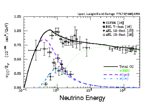
Figure 6.1: Charged current neutrino cross section contributions as a function of neutrino energy (in GeV): quasi-elastic (dashed), resonant single pion (dot-dash), and deep inelastic scattering (dotted) processes. Figure extracted from [76].

At energies near $\sim 1$ GeV, neutrino interactions are predominantly quasi-elastic (QE) and resonant single pion production; each are known to the $10-20\%$ level from light target ($H_{2}$, $D_{2}$) neutrino data. Although deep inelastic scattering (DIS) processes have been measured with impressive precision ($<2\%$) at high energies, it is challenging both to measure and to model neutrino interactions at low energies, where there is substantial overlap between various poorly-understood contributing processes.

Furthermore, because modern neutrino oscillation detectors consist of heavy nuclei ($C$, $O$, $Ar$, $Fe$, $Pb$), the complex target adds additional complications. In this case, one must deal with the effects of Pauli blocking, Fermi motion of the target nucleons, and final state interactions (i.e. careful accounting for the fact that the outgoing hadron may reinteract before exiting the nucleus). Final state effects (nuclear reinteractions, $\pi$ absorption, and charge exchange) often dominate; they can vary depending on the neutrino process, and certainly have not been disentangled experimentally. Nuclear effects significantly impact both the rate and kinematics of the neutrino reaction, as well as the observed final state event composition and multiplicity (see, for example, Section 3.2). Although nuclear effects have been studied extensively using muon and electron beams, no comparable effort has been made using neutrinos. Neutrino cross sections have been measured on nuclear targets in the past, but these experiments suffered from low statistics and typically published only free nucleon cross sections. By making dedicated, high statistics measurements of neutrino interaction cross sections on a scintillator-based target, FINeSSE could greatly improve the current experimental situation.

Several efforts are already underway to more precisely measure neutrino interactions on nuclei at low energy. Measurements of NC $\pi^{0}$/QE and inelastic/QE event ratios have been performed in the K2K water Čerenkov and scintillator-based fine grain near detectors, respectively [77]. These measurements exhibit $\sim 10\%$ accuracy based on samples of roughly 5,000-10,000 events [78]. Although MiniBooNE can additionally offer improved cross section constraints with increased statistics over the K2K near detector ensemble, such Čerenkov-based detection methods are inherently limited in their capabilities. The ability to disentangle the various channels (QE, resonant, coherent, DIS, etc.) in a nuclear environment necessitates use of a fine-grained detector such as that being proposed for FINeSSE.

6.1.2 Prospects for Measuring Cross Sections at FINeSSE

The following subsections outline prospects for several exclusive neutrino cross section measurements at FINeSSE. This includes improved constraints on NC $\pi^{0}$ production and strange particle production.

Neutral Current $\pi^{0}$ Production

The dominant backgrounds to $\mbox{$\nu_{\mu}$}\rightarrow\mbox{$\nu_{e}$}$ appearance searches result from two principal sources: the intrinsic $\nu_{e}$ component in the beam and NC $\pi^{0}$ production where the final state is misclassified as an electron. Experiments primarily rely on Monte Carlo simulations to estimate their $\pi^{0}$ backgrounds. Such simulations must model several mechanisms for producing a single $\pi^{0}$: resonance production, coherent single pion production, and deep inelastic scattering in which additional hadrons are absorbed in the nuclear medium before being detected. The dominant means of single pion production at low energy arises through this first production mechanism: excitation of baryon resonances ($\Delta,N$) that decay as:

$$\mbox{$\nu_{\mu}$}\,N\rightarrow l\, N^{*}$$

$$N^{*} \rightarrow\pi\,N^{\prime}~{}.$$

As a result, there are seven such resonant neutrino reaction channels: three charged current and four neutral current:

$$\mbox{$\nu_{\mu}$}\,p \rightarrow \mu^{-}\,p\,\pi^{+}$$

$$\mbox{$\nu_{\mu}$}\,n \rightarrow \mu^{-}\,n\,\pi^{+}$$

$$\mbox{$\nu_{\mu}$}\,n \rightarrow \mu^{-}\,p\,\pi^{0}$$

$$\mbox{$\nu_{\mu}$}\,p \rightarrow \mbox{$\nu_{\mu}$}\,n\,\pi^{+}$$

$$\mbox{$\nu_{\mu}$}\,p \rightarrow \mbox{$\nu_{\mu}$}\,p\,\pi^{0}$$

$$\mbox{$\nu_{\mu}$}\,n \rightarrow \mbox{$\nu_{\mu}$}\,n\,\pi^{0}$$

$$\mbox{$\nu_{\mu}$}\,n \rightarrow \mbox{$\nu_{\mu}$}\,p\,\pi^{-}$$

Traditionally, Monte Carlo simulations covering the low energy region have used theoretical calculations by Rein and Sehgal [79] to predict the rate and kinematics of neutrino resonance production. Such models are tuned to reproduce neutrino single pion data, but remain poorly constrained, because of the limited availability and large uncertainties in existing experimental data. As an example, Figure 6.2 shows the experimental constraints on single $\pi^{0}$ production from charged current (CC) neutrino data. Note that all of the data at low energy were collected from light targets.

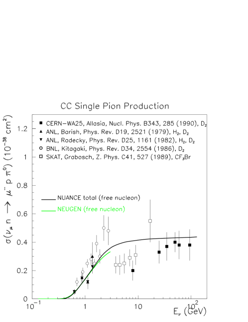
Figure 6.2: Measurements of the CC resonant single $\pi^{0}$ cross section, $\sigma(\mbox{$\nu_{\mu}$}\,n\rightarrow\mu^{-}\,p\,\pi^{0})$. Also shown are the Rein and Sehgal-based predictions from two publicly available Monte Carlo generators [80].

By contrast, Figure 6.3 shows the only available experimental measurement of an absolute resonant NC $\pi^{0}$ cross section. These NC data result from a recent reanalysis of Gargamelle bubble chamber data at 2 GeV [81]. Because the NC cross sections are less well known, experiments typically in practice assign large $25-30\%$ uncertainties to NC resonant production processes.

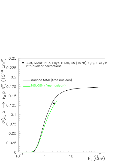
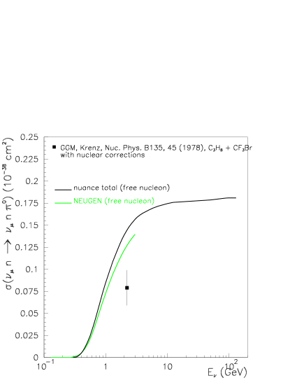
Figure 6.3: NC resonant single $\pi^{0}$ cross sections, $\sigma(\mbox{$\nu_{\mu}$}\,p\rightarrow\mbox{$\nu_{\mu}$}\,p\,\pi^{0})$ (left) and $\sigma(\mbox{$\nu_{\mu}$}\,n\rightarrow\mbox{$\nu_{\mu}$}\,n\,\pi^{0})$ (right). Also shown are the Monte Carlo predictions from [80].

The data are even more sparse for the other contributing production mechanism, coherent single pion production. In coherent interactions, neutrinos scatter off the entire nucleus rather than its individual constituents. Because of the negligible energy transfer to the target nucleus ($A$), such processes distinctly provide a single forward scattered pion. Like in the resonant case, both NC and CC processes are possible:

$$\mbox{$\nu_{\mu}$}\,A \rightarrow \mbox{$\nu_{\mu}$}A\,\pi^{0}$$

$$\mbox{$\nu_{\mu}$}\,A \rightarrow \mu^{-}A\,\pi^{+}$$

Almost all current Monte Carlo simulations implement Rein and Sehgal’s calculation [85] of coherent pion production cross sections and kinematics. While such predictions have been constrained by numerous experimental measurements at high energy [82], the lowest energy data available is at 2 GeV on an aluminum spark chamber target [83]. Figure 6.4 shows the low energy Aachen measurement compared to several model calculations.

Figure 6.4: Experimental measurement of the NC coherent $\pi^{0}$ production cross section at low energy compared to current model predictions [84],[85].

The most recent calculations [84] yield a factor of two to six less coherent pion production at these energies than the earlier Rein and Sehgal based predictions [85]. Because of the lack of low energy experimental data and the existence of several conflicting theoretical predictions, oscillation experiments typically assign a $100\%$ uncertainty to coherent processes. This large uncertainty is especially important because coherent production may comprise up to $20\%$ of the overall NC $\pi^{0}$ rate. The ability to further constrain NC $\pi^{0}$ production at low energies would thus be of great use in achieving increased sensitivity to $\mbox{$\nu_{\mu}$}\rightarrow\mbox{$\nu_{e}$}$ oscillations, and in placing more stringent limits on the oscillation of standard neutrinos to sterile states.

In two years of running, FINeSSE will collect a total sample of $\sim 20,000$ NC $\pi^{0}$ resonant events and over 5,000 NC coherent $\pi^{0}$ interactions. In addition, FINeSSE’s superior energy resolution and event reconstruction capabilities will greatly enhance the ability to select $\pi^{0}$ interactions. Figures 6.5 and 6.7 show simulated NC resonant $\pi^{0}$ events in the FINeSSE detector. A $\mbox{$\nu_{\mu}$}\,p\rightarrow\mbox{$\nu_{\mu}$}\,p\,\pi^{0}$ interaction (Figure 6.5) can be distinguished by the presence of three separated energy deposits corresponding to the final state proton and the two photons emitted from $\pi^{0}\rightarrow\gamma\,\gamma$. A charged current $\pi^{0}$ event, $\mbox{$\nu_{\mu}$}\,n\rightarrow\mu^{-}\,p\,\pi^{0}$, (Figure 6.6) is additionally accompanied by a final state muon track. In contrast, a $\mbox{$\nu_{\mu}$}\,n\rightarrow\mbox{$\nu_{\mu}$}\,n\,\pi^{0}$ interaction (Figure 6.7) can only be produced by scattering from carbon, and will contain only two clusters of hits corresponding to the two photons from the $\pi^{0}$ decay. NC coherent $\pi^{0}$ events (Figure 6.8) are similar in signature to the former class of events; however, in this case, the energies and angles of the two final state photons can be used to determine if the $\pi^{0}$ angular distribution is more forward peaked as one expects for coherent scattering.

     

Figure 6.5: Hit-level simulations of NC $\pi^{0}$ interactions in the FINeSSE detector, $\mbox{$\nu_{\mu}$}\,p\rightarrow\mbox{$\nu_{\mu}$}\,p\,\pi^{0}$. The three hit clusters correspond to the final state proton and two photons from $\pi^{0}\rightarrow\gamma\,\gamma$.

       

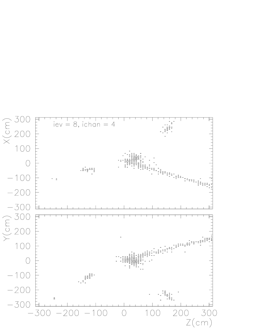
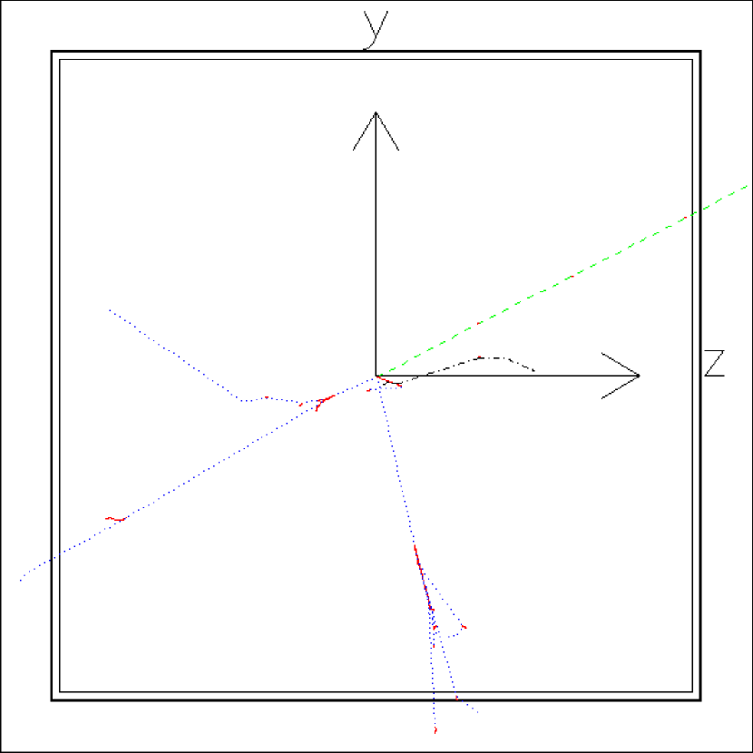
Figure 6.6: A $\mbox{$\nu_{\mu}$}\,n\rightarrow\mu^{-}\,p\,\pi^{0}$ CC $\pi^{0}$ interaction in the FINeSSE detector. The right hand figure shows the true GEANT particle trajectories in the YZ plane. In this case, a muon is produced in addition to the three hit clusters from the proton and two photons.

     

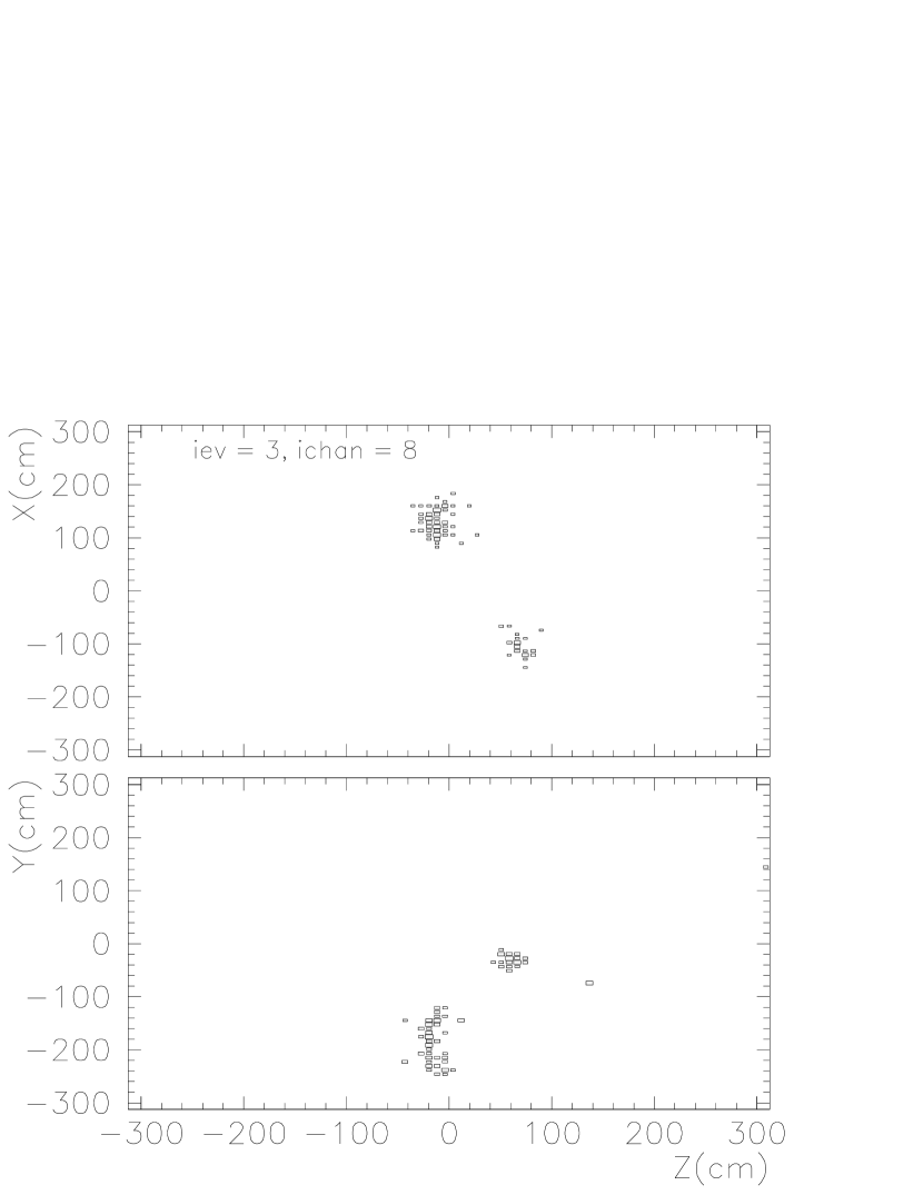
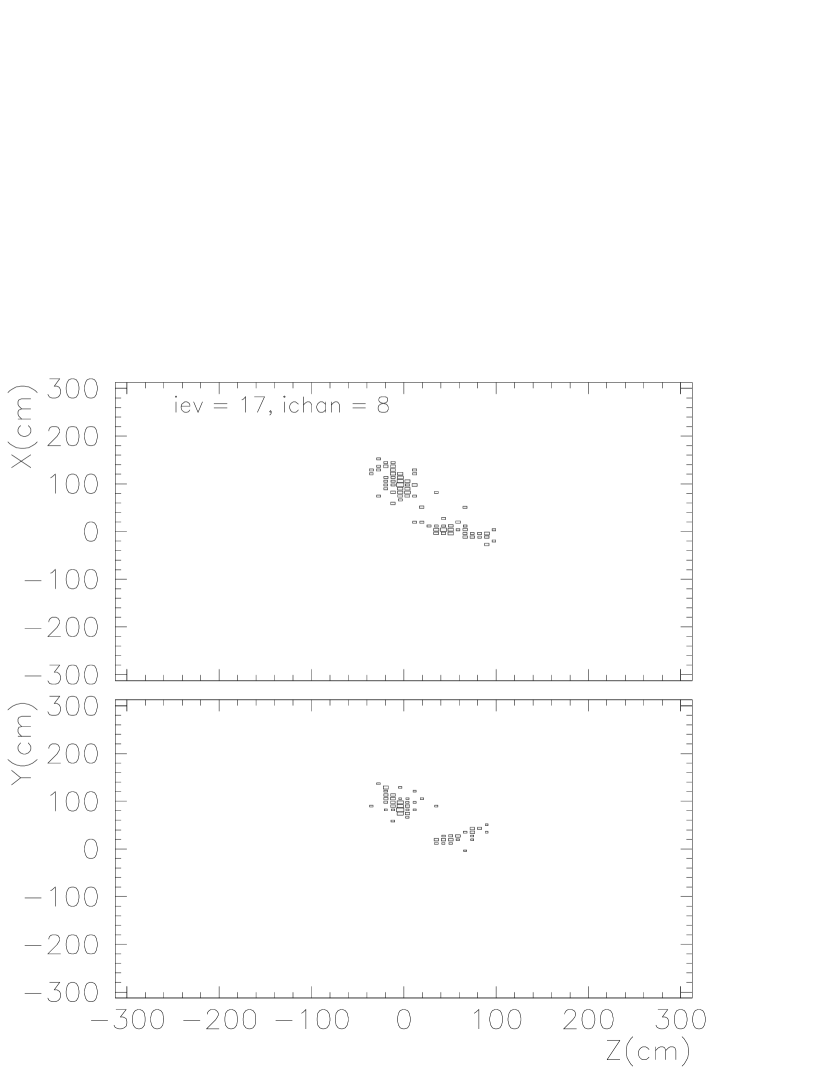
Figure 6.7: Two NC $\pi^{0}$ interactions in the FINeSSE detector, $\mbox{$\nu_{\mu}$}\,n\rightarrow\mbox{$\nu_{\mu}$}\,n\,\pi^{0}$. The separated hit clusters correspond to the two photons emitted from the $\pi^{0}$ decay.

       

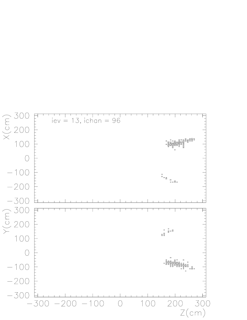
Figure 6.8: A NC coherent $\pi^{0}$ interaction in the FINeSSE detector, $\mbox{$\nu_{\mu}$}\,^{12}C\rightarrow\mbox{$\nu_{\mu}$}\,^{12}C\,\pi^{0}$. The figure on the right shows the true GEANT particle trajectories in the XZ plane for the same event. As can be seen, the hit clusters correspond to the two photons from the $\pi^{0}$ decay.

While such events leave distinct signatures in the FINeSSE detector, determining the efficiency and accuracy with which FINeSSE can measure $\pi^{0}$ rates and kinematics will require development of a cluster algorithm and tracker designed to located gaps in energy deposits. While not yet optimized, preliminary studies have demonstrated that $\pi^{0}$ efficiencies and purities can be obtained that surpass those achieved with either the MiniBooNE or K2K Čerenkov–based detectors. Given that the largest sources of error arise from nuclear uncertainties, by measuring $\pi^{0}$ production on carbon, FINeSSE should therefore be able to reduce the currently assigned NC $\pi^{0}$ production uncertainty (Section 6.1.2) by as much as a factor of two.

In its ability to isolate $\pi^{0}$ interactions, FINeSSE has an especially important role to play given that there is currently no NC $\pi^{0}$ data on nuclear targets below 2 GeV, and only low energy CC $\pi^{0}$ data measured on deuterium targets. FINeSSE is well-positioned to be the first neutrino experiment to measure NC $\pi^{0}$ (and CC $\pi^{0}$) production on carbon at these energies ($<E_{\nu}>\sim 700$ MeV), thus providing an important constraint to oscillation experiments such as MiniBooNE, as well as to other accelerator- and atmospheric-based $\nu_{e}$ appearance experiments employing heavy nuclear targets. Such efforts at FINeSSE are also complementary to slightly higher energy ($<E_{\nu}>\sim 1.3$ GeV) scintillator-based analyses currently being planned after upgrades to the K2K near detector site [86].

Strange Particle Production

Proton decay modes containing a final state kaon, $p\rightarrow\nu K^{+}$, have large branching ratios in many SUSY GUT models. Because there is a non-zero probability that an atmospheric neutrino interaction can mimic a proton decay signature,

$$\mbox{$\nu_{\mu}$}\,n\rightarrow\mu^{-}\,K^{+}\,\Lambda$$

$$\mbox{$\nu_{\mu}$}\,p\rightarrow\mbox{$\nu_{\mu}$}\,K^{+}\,\Lambda,$$

it is important to reliably estimate this background. Present uncertainties on this background process are as large as $100\%$ [87] both because neutrino strange particle production rates have been measured in only a few experiments, and because there are not many predictive theoretical models [88]. Figure 6.9 shows the only two experiments which have published cross sections on the dominant associated production channel, $\mbox{$\nu_{\mu}$}n\rightarrow\mu^{-}K^{+}\Lambda$. Both measurements were made on a deuterium target and based on less than 30 events combined.

Figure 6.9: Experimental measurements of the $\mbox{$\nu_{\mu}$}n\rightarrow\mu^{-}K^{+}\Lambda$ cross section. Also shown are the predictions from two publicly available Monte Carlo generators [80].

Based on NUANCE Monte Carlo predictions, approximately 90 such interactions are expected at FINeSSE in two years of running. The ability to identify and isolate neutrino production of strange particles at FINeSSE would be of even larger importance to proton decay searches, not only because of potentially large event samples, but also because these interactions will be taking place at energies near threshold and on a nuclear target, both of which are particularly relevant for present and future proton decay studies. Identifying such events at FINeSSE will certainly be challenging. Although the event signature is complex, it is potentially very distinctive. Roughly $64\%$ of the time, a typical CC kaon event will contain two oppositely charged muons, one from the primary neutrino interaction and the other from $K$ decay, $K^{+}\rightarrow\mu^{+}\mbox{$\nu_{\mu}$}$ (Figure 6.10). In addition, since most of the kaons will stop and decay at rest, the $\mu^{+}$ is monoenergetic with a momentum of $\sim 240$ MeV, and will appear roughly 12 ns after the initial interaction.

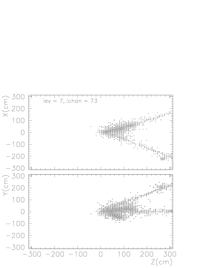
Figure 6.10: Example of a $\mbox{$\nu_{\mu}$}\,n\rightarrow\mu^{-}\,K^{+}\,\Lambda$ event in the FINeSSE detector. In this event, the associated strange particles decayed yielding a hadronic shower and second muon: $\Lambda\rightarrow p\,\pi^{-}$ (BR=$63\%$) and $K^{+}\rightarrow\mu^{+}\mbox{$\nu_{\mu}$}$ (BR=$64\%$).

Further studies must assess FINeSSE’s multi-track reconstruction capabilities and DIS backgrounds before any stringent limits on strange particle production can be set. However, such a possibility should be seriously explored as FINeSSE could potentially be the first experiment to measure this reaction both near threshold and on a nuclear target.

6.2 Neutrino Electron Scattering: Neutrino Magnetic Moment

In the Standard Model, massive, charged particles have intrinsic magnetic moments by virtue of their spin. If we introduce neutrino mass into the theory, an effective neutrino magnetic moment can arise. How neutrino mass fits into the Standard Model, be it via a standard Dirac mechanism, SUSY, or something else, affects the size and origin of this magnetic moment. Thus, we can use a neutrino magnetic moment measurement to tell us about how neutrinos fit into the larger theory.

In the minimally extended Standard Model, massive Dirac neutrinos of mass $m_{\nu}$ can have a neutrino magnetic moment of:

$$\mu_{\nu}=\frac{3eG_{F}}{8\sqrt{2}\pi^{2}}m_{\nu}\sim 3\times 10^{-19}\mu_{B}\left(\frac{m_{\nu}}{1{\rm eV}}\right)~{},$$ (6.1)

arising from one loop radiative corrections in diagrams with W-boson exchange as in Figure 6.11.

We can place neutrinos with non-zero magnetic moments in the context of a larger theory such as SUSY and Extra Dimensions. These extensions to the Standard Model such as the super symmetric left-right model predict larger neutrino magnetic moments of the size [89]

Figure 6.11: One loop radiative correction diagram with a massive neutrino.

$$\mu_{\nu_{e}}\cong 5\times 10^{-15}-10^{-16}\mu_{B}$$ (6.2)

$$\mu_{\nu_{\mu}}\cong 1\times 10^{-12}-10^{-13}\mu_{B}$$ (6.3)

$$\mu_{\nu_{\tau}}\cong 2\times 10^{-12}\mu_{B}.$$ (6.4)

Theories involving Extra Dimensions produce an effective neutrino magnetic moment as large as $10^{-11}\mu_{B}$  [90].

A non-zero neutrino magnetic moment would also have important implications in cosmology in the development of stellar models. Astrophysical limits such as plasmon, or photon wave packets, decay rates from horizontal branch stars and neutrino energy loss rate from supernovae allow a neutrino magnetic moment as large as $10^{-11}\mu_{B}$ [91, 92, 93].

The most straightforward way to look for a non-zero neutrino magnetic moment is via an excess in $\nu-e$ scattering:

$$\mbox{$\nu_{\mu}$}\,e^{-}\rightarrow\mbox{$\nu_{\mu}$}\,e^{-}~{}.$$

A non-zero neutrino magnetic moment will give rise to an electromagnetic contribution to this process in addition to the Standard Model Z exchange. This electromagnetic contribution to the cross section for neutrino-electron elastic scattering is of the form:

$$\sigma_{EM}=f^{2}\pi r_{0}^{2}\left[\frac{T_{e}^{\rm min}}{E_{\nu}}-ln\left(\frac{T_{e}^{\rm min}}{E_{\nu}}\right)-1\right]~{},$$ (6.5)

where $r_{0}$ is the classical electron radius, $T_{e}^{\rm min}$ is the minimum kinetic energy of the recoil electron, $E_{\nu}$ is the neutrino energy, and $f$ is the neutrino magnetic moment in units of Bohr magnetons.

At low $y=T_{e}/E_{\nu}$, the electromagnetic contribution to the neutrino-electron cross section increases rapidly, while the Standard Model contribution increases only gradually. The resulting shape dependence in the differential cross section can be used to look for a signal in a high statistics experiment like FINeSSE. The differential cross section contributions for weak and electromagnetic components of the neutrino-electron elastic scattering cross section are given by:

$$\frac{d\sigma^{weak}}{dT_{e}}=\frac{2m_{e}G_{F}^{2}}{\pi}\left[g_{L}^{2}+g_{R}^{2}\left(1-\frac{T_{e}}{E_{\nu}}\right)^{2}-g_{R}g_{L}\frac{m_{e}}{E_{\nu}}\frac{T_{e}}{E_{\nu}}\right]~{},~{}{\mathrm{and}}$$ (6.6)

$$\frac{d\sigma^{EM}}{dT_{e}}=\frac{\pi\alpha^{2}\mu_{\nu}^{2}}{m_{e}^{2}}\left(\frac{1}{T_{e}}-\frac{1}{E_{\nu}}\right)~{},$$ (6.7)

where $T_{e}$ is the electron recoil energy and $E_{\nu}$ is the neutrino energy.

Present limits set on neutrino magnetic moments are many orders of magnitude away from the Standard Model prediction including massive Dirac neutrinos. They are, however, only one to two orders of magnitude away from predictions from certain beyond-the-Standard-Model theories and astrophysical limits. The most stringent limits set by experiments for neutrino magnetic moments for each neutrino flavor are listed in Table 6.1. The experimental limit for the muon-neutrino magnetic moment coming from the LSND experiment is an upper limit of $\mu_{\nu_{\mu}}<6.8\times 10^{-10}\mu_{B}$ [94] set by measuring the total neutrino-electron elastic scattering cross section. An improved limit by about a factor of two, on the muon neutrino magnetic moment is expected from MiniBooNE  [99].

$\nu$ Flavor	Limit Set($\mu_{B}$)	Experimental Data	Process	Reference
$\nu_{e}$	$1.5\times 10^{-10}$	Super Kamiokande	shape of differential cross section	[95]
$\overline{\nu_{e}}$	$1.8\times 10^{-10}$	combination of $\overline{\nu_{e}}$ reactor experiments	excess in total cross section	[96, 97]
$\nu_{\mu}$	$6.8\times 10^{-10}$	LSND	excess in total cross section	[94]
$\nu_{\tau}$	$5.4\times 10^{-7}$	DONUT	excess in total cross section	[98]

Table 6.1: Limits set on neutrino magnetic moments.

Number of events and, more importantly, low energy threshold for electron recoil, determine how sensitive an experiment is to a non-zero neutrino magnetic moment. FINeSSE expects a number of $\nu-e$ scattering events (86 events) comparable to the number MiniBooNE will see (101 events). FINeSSE can improve upon MiniBooNE’s expected measurement in identifying events at low electron recoil energy, where the differential cross section is most sensitive to a non-zero neutrino magnetic moment. Figure 6.12 shows a typical $\nu-e$ interaction in FINeSSE’s Vertex Detector. These events are very forward and have a very distinctive shower shape. The granularity of the Vertex Detector as compared to the MiniBooNE detector may allow FINeSSE to clearly identify these lowest energy events via a shower shape analysis. This would provide better sensitivity to non-zero muon neutrino magnetic moment than any previous experiment.

       

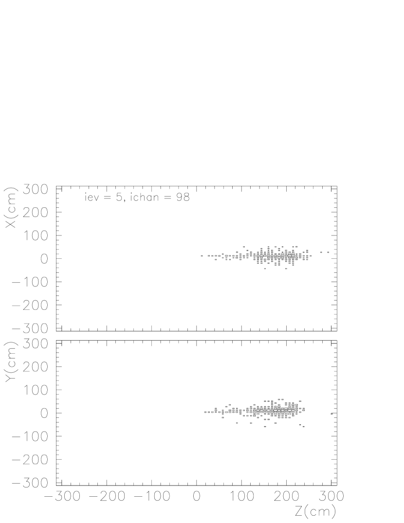
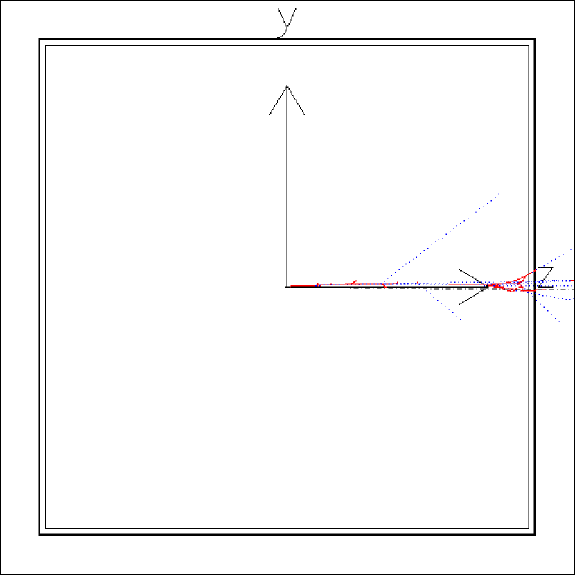
Figure 6.12: A $\mbox{$\nu_{\mu}$}\,e^{-}\rightarrow\mbox{$\nu_{\mu}$}\,e^{-}$ elastic scattering interaction in the FINeSSE detector. The figure on the right shows the true electron shower in GEANT for the same event. Such events characteristically contain a single forward scattered electron.

6.3 Antineutrino Running and $\Delta s$

If the opportunity arises to run FINeSSE with an antineutrino beam, there are some features of $\bar{\nu}p\rightarrow\bar{\nu}p$ scattering that would make this channel exciting to investigate. The ratio in the antineutrino channel is actually slightly more sensitive to $\Delta s$ than for neutrinos. This can be seen in Figure 6.13a-b, where the relative change in the ratio with the same change in $\Delta s$ is larger for antineutrinos than for neutrinos. In addition, the change in the ratio as a function of $Q^{2}$ is different for antineutrinos. This would allow a simultaneous extraction of $\Delta s$ and $M_{A}$, since (see Figure 6.13) the ratio has a much different behavior in $Q^{2}$ for different values of $M_{A}$ in $\bar{\nu}p\rightarrow\bar{\nu}p$.

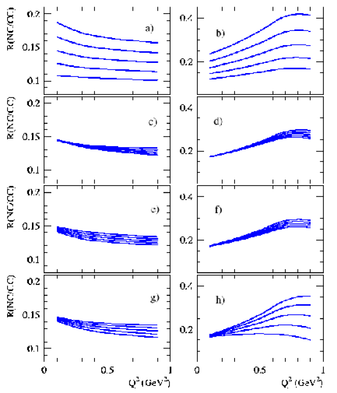
Figure 6.13: The ratio of NC to CC scattering for neutrinos (left column of plots) and antineutrinos (right column) as a function of $Q^{2}$. In each of the 4 rows one of the form factors is varied. In a-b) $-0.2<\Delta s<+0.2$, c-d) $-0.2<F_{1}^{s}<+0.2$, e-f) $0.95<M_{A}<1.15$ GeV/c².

6.4 Long-term Running of FINeSSE+MiniBooNE

If MiniBooNE sees a signal and it is confirmed by both phase II MiniBooNE and FINeSSE+MiniBooNE cross checks, Fermilab is likely to continue the 8 GeV program. The natural next step is the installation of BooNE, the multi-detector experiment planned as the upgrade to MiniBooNE. Given that BooNE is in the planning stages, it is unclear when this program would begin. However, it is safe to say that it is unlikely that BooNE can be fully constructed and running before 2010. During this construction period, it would make sense to continue running FINeSSE+MiniBooNE.

In this section, we consider what can be achieved if FINeSSE+MiniBooNE receives $3\times 10^{21}$ protons on target before the BooNE detector system is inaugurated. This is based on the premise that upgrades to the Booster can allow the 8 GeV line to return to the level of $1\times 10^{21}$ protons/year near the end of the decade. To be clear, we are not requesting approval for this scenario from the PAC. We are simply using this to illustrate the long-term value of the FINeSSE detector.

In this case, the statistics limited measurements described in the previous section can be greatly improved. We believe we can reasonably achieve the systematic errors listed in Table 6.2.

NC $\pi^{0}$:	0.03
Radiative $\Delta$ Decay:	0.06
$\nu_{e}$ from $\mu$:	0.04
$\nu_{e}$ from $K^{+}$:	0.04
$\nu_{e}$ from $K^{0}$:	0.06

Table 6.2: Systematic errors for the (hypothetical) scenario of $3\times 10^{21}$ POT.

At this point MiniBooNE will have acquired $4\times 10^{21}$ protons on target (25% with the 50 m absorber and 75% with the 25 m absorber). The capability of such a measurement is shown in Figure 6.14. The colored regions show the LSND allowed range. The solid ellipses indicates the 1$\sigma$ measurement capability for the oscillation parameters at two possible true $\Delta m^{2}$ values. For comparison, the capability from MiniBooNE phase I running is indicated by the dashed ellipses.

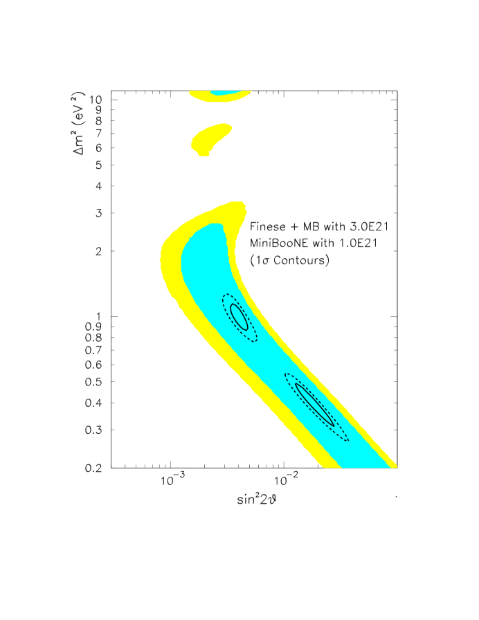
Figure 6.14: The solid ellipse shows the 1$\sigma$ measurement capability for two sets of oscillation parameters for FINeSSE+MiniBooNE for $3\times 10^{21}$ POT. The dashed ellipse shows the MiniBooNE Phase I capability. The colored segments indicate the LSND-allowed regions.

Chapter 7 Overview of Cost and Schedule

The FINeSSE detector cost is estimated to be $2.25 M ($2.8 M with contingency). These estimates do not include EDIA or indirect costs. Funding for the detector will come from the university funding agencies. EDIA and indirect costs will be added as appropriate when the funding structure is in place, and will account for differences in each university’s accounting practices.

The FINeSSE enclosure cost is estimated to be $800K ($1.6 M including contractor O&H, EDIA, management reserve, and indirect costs) as determined through a Preliminary Design Report written by the Fermilab Facilities Engineering Section (FESS). See Appendix B which contains this report.

The dimensions of the enclosure were chosen to comfortably contain the detector and provide adequate working room around the detector. There is also adequate room for detector installation. The FINeSSE schedule incorporates detector and enclosure design, construction, and installation over the next two years, with data taking scheduled to begin in mid-2006.

The following sections provide breakdown of detector costs, enclosure costs, construction and installation schedule, and an overview of the FINeSSE schedule from now until the beginning of the FINeSSE physics run.

7.1 Detector and Enclosure Costs

The FINeSSE detector is comprised of two subdetectors (cf. Chapter 4): the Vertex Detector, followed downstream by the Muon Rangestack. Table 7.1 lists preliminary costing of the components of these detectors, as well as total costs.

The cost of the detector is driven mainly by PMT and electronics costs that combined total $900,000. The vertex detector tank that holds the scintillator, fiber, and PMTs is about $265,000. The remaining costs are for fiber, scintillator, and oil. The cost driver for the Rangestack detector is the iron planes, costing $327,000. Most of this cost comes from fabrication. An additional cost of about $100,000 is set aside for rigging and installation of the detector.

Contingency is applied to the total detector costs. EDIA and indirect costs are not included, as it is expected that the majority of these costs will come through university groups, where EDIA and indirect costs are treated differently by each university. These costs will be included once the funding profile by universities is established.

The detector enclosure design went through a series of studies within FESS. To meet the requirements of detector construction and operation, several enclosure options were studied. They are summarized in the Alternate Comparison Matrix given in Appendix B. The options ranged in cost from $1.48M to $2.54M. The study compared the use of a gantry crane to a bridge crane, a hatch cover to a pre-engineered building, and a sheet pile pit to a secant pile pit. The chosen option includes a sheet pile pit, a hatch cover, and a gantry crane for about $1.6M. If a mobile crane were used, rather than a gantry crane, the construction cost could be reduced to $1.48M, but this would be offset by the operational costs of crane rental during the detector installation phase. There will be no need for crane coverage once the detector is installed and operating. A cross-sectional view of the enclosure is shown in Figure 4 of the Appendix, and the plan view is given in Figure 3.

7.2 Schedule

The FINeSSE schedule allows for 2.5 years for enclosure and detector construction and installation, with the start of the physics run beginning in mid-2006. The FINeSSE schedule for enclosure construction calls for construction of the building to commence in mid to late 2004. Total time to construct this enclosure is about six months, as described in detail in Appendix B, keeping FINeSSE on schedule for detector installation beginning in mid-2005. Detector construction and installation is expected to take 1.5 years.

FINeSSE is on an aggressive but achievable schedule for a number of reasons. First, FINeSSE physics is important and timely and should be pursued as quickly as possible. Second, there is an existing, running neutrino beamline which should be utilized as much as possible. Finally, the FINeSSE physics run is timed to coincide with the end of MiniBooNE antineutrino running and fits well with the MiniBooNE schedule. The FINeSSE schedule, up to the start of our physics run in mid-2006, is shown in Figure 7.1.

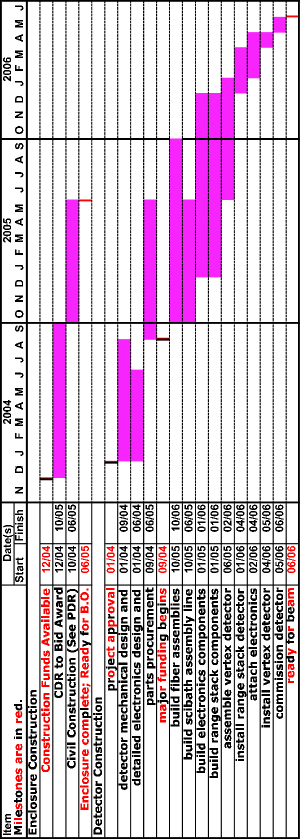
Figure 7.1: The FINeSSE schedule, showing the milestones from winter 2004 until beam can be taken in 2006. Milestones are shown in red.

Chapter 8 Conclusions

We propose to construct and operate a novel neutrino detector to run in the Booster neutrino beamline, 100 m from the Booster neutrino production target. The physics motivation for this experiment is twofold.

First, we will measure the strange spin of the proton $\Delta s$ using a theoretically robust method, an intense, low energy neutrino beam, and a novel detection technique. Second, FINeSSE will look for $\nu_{\mu}$ disappearance, in conjunction with MiniBooNE, at high $\Delta m^{2}$ in an astrophysically interesting region.

FINeSSE will achieve these physics goals using a two-part detector to measure both short, low energy proton tracks and longer, muon tracks. Low energy proton tracks will be well measured in a, liquid scintillator “bubble chamber”. Downstream of this Vertex Detector is a Muon Rangestack designed to range out higher energy muons that are not contained in the Vertex Detector.

FINeSSE requires 6$\times 10^{20}$ POT total to reach its physics goals. In the NuMI era, these protons can be delivered over a two year period.

Appendix A Vertex Detector Design Studies

In determining the best detector design to address the FINeSSE physics goals, a number of options were considered. In addition to the “Scibath” design described in Chapter  4, we studied a design called “Scistack”, much like the K2K Scibar detector [61]. We found this detector was not optimal for identifying low energy proton tracks from $\nu-p$ elastic scatters, crucial for the $\Delta s$ analysis. By contrast, the Scibath option did not have these limitations. This appendix describes these Scistack studies including building and testing of a prototype detector, Monte Carlo studies, and conclusions.

A.1 Scistack design, Feasibility and Cost

The Scistack detector is a 2.5 $m^{3}$ volume of scintillating plastic bars. The 2 cm $\times$1 cm extruded polystyrene bars are co-extruded with a TiO₂ outer layer for reflectivity, and a hole down the center for a WLS fiber. Bars are organized in planes normal to the beam direction with bars in even-numbered planes oriented in the x direction and bars in odd number planes oriented in the y direction. This design has a total of 31250 bars and associated readout channels. Readout is identical to the Scibath design with light piped out via WLS fibers, and recorded and digitized as described in Section 4.1.3.

The cost of a Scistack detector is comparable to the Scibath detector. Plastic and liquid scintillator as well as WLS fiber are comparable in both detectors. A cost driver for both detectors is channel cost. The number of channels in this design is larger by a factor of 1.5. This is offset by employing channel multiplexing which decreases the channel cost by a factor of eight. However, channel multiplexing can be accommodated only with 16 anode MAPMTs (as opposed to the Scibath 64 anode MAPMTs) due to physical size of each anode, driving the cost per channel back up. Cost of WLS fiber also increases in Scistack as there are 1.5 more channels; this, however, is not a significant cost overall. Folding in all cost differences, costs for the two detectors are comparable.

A.2 Prototype testing

A small prototype of the Scistack detector was designed, constructed, and tested during the summer of 2003. The prototype design, shown in Figure A.1 consists of a ten by three stack of 2 cm $\times$ 1 cm scintillator bars, with a WLS fiber inserted down the center of each. The fiber is attached to 16 anode MaPMTs and read out through the same electronics used for the Scibath prototype tests, described in Chapter 4. The Scistack prototype was exposed to the IUCF proton beam, as was Scibath (again, see Chapter 4). Scistack performed as expected. Light output increased as the proton beam moved, normal to the bars, and closer to the readout. Tracks were easily seen, as expected, as the proton beam traversed the stack both with the stack oriented normal to the beam and at an angle with respect to the beam. This detector employs known technology; there were no surprises.

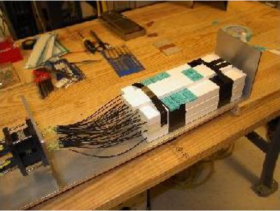
Figure A.1: Photograph of the Scistack prototype. Scintillator bars are stacked in a 10 x 3 array. WLS fiber, polished on both ends, routed through each bar, is read out on one end by Hamamatsu 16 anode MaPMTs. The entire prototype is housed in a light tight aluminum box with connections for Lemo and high voltage. The box is built on a rotatable stand to facilitate testing in the IUCF beam.

A.3 Monte Carlo Studies

While the detection techniques proved acceptable experimentally, Scistack Monte Carlo work revealed a feature in the detector geometry which makes this detector unsuitable for FINeSSE’s $\Delta s$ measurement.

The design goal of the FINeSSE Vertex Detector is to be able to cleanly identify and measure low energy protons from $\nu-p$ elastic scatters. Scistack Monte Carlo work shows that these very events, most important to the $\Delta s$ analysis, are frequently not reconstructible in Scistack due to limitations in tracking in this detector. Specifically, low $Q^{2}$ events tend to be directed at high angles with respect to the beam direction. The Scistack detector reconstructs these events with less success, since bars are oriented normal to the beam direction, and therefore in the same direction as these low $Q^{2}$ events. The Monte Carlo and these studies are described below.

A.3.1 Scistack Monte Carlo

The GEANT-based Monte Carlo for the Scistack option is designed to be identical to the Scibath option except for the configuration of the central detector. This includes the output ntuple which has the same format, with appropriate changes in the meaning of the variables, to minimize differences in the reconstruction program.

The central detector for Scistack consists of 250 layers, each 1 cm thick, along the beam axis ($z$). Each layer has 125 scintillator bars, 2 cm in the transverse direction, with the bars in alternating layers aligned along the $x$ and $y$ axes. Each 1 cm by 2 cm by 2.5 m bar has a 1.5 mm OD wavelength shifting optical fiber along its axis, to capture and transmit photons from the scintillator to the PMTs. The outer 0.5 mm of each bar is a TiO₂ wrapper which optically isolates the bars. The highly reflective inner surface of the wrapper increases the light capture in the fibers by approximately a factor of two. The scintillator has an attenuation length of 5.0 m.

After allowing for fiber capture and transmission efficiencies, assumed to be the same as Scibath, each photon entering a fiber has its layer and bar number recorded in the output ntuple. The actual capture efficiency as well as the number of photons generated per MeV of energy loss would be higher in Scistack than in Scibath. But the number of photons detected is so large that this is not an important factor in the current studies.

The resulting ntuple is reconstructed by the same Hough transform method used for Scibath, and the results are used to determine the angular and energy resolution of Scistack as well as its particle identification capabilities. The Monte Carlo samples generated for these studies include single electrons, muons, nucleons, pions, and kaons with kinetic energies between 0 and 500 MeV, generated isotropically in direction. We also ran a large sample of neutrino interactions generated using NUANCE. Each sample was run with vertices near the center of the detector, and again with vertices spread uniformly throughout the detector. The results are discussed in the following section.

A.3.2 $\nu-p$ Sample in Scistack

Neutrino-proton elastic scatters at low energies produce short-track, low energy protons. Samples of protons generated and reconstructed as described above were studied to determine if the Scistack detector was suitable for this measurement. Figure A.2 shows the number of tracks reconstructed as a function of true kinetic energy for this sample. As is indicated, tracks below 150 MeV tend not to be reconstructible. These tracks tend to be at high angle and therefore traversed few bars. Figure A.3 show reconstructed tracks as a function of true kinetic energy and angle for both Scitrack and Scibath.

The neutrino interaction sample generated with NUANCE was used to understand the Scistack efficiency as compared to Scibath. Similar cuts as were applied to the reconstructed Scibath events to extract a NCp sample, were applied to the Scistack sample. The inability to reconstruct the proton events described above, translated into a more than 30% decrease in $\nu-p$ statistics in the 0.2$<Q^{2}<$0.4 bin, the crucial energy bin for the $\Delta s$ analysis.

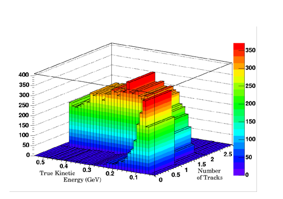
Figure A.2: Number of tracks reconstructed versus true kinetic energy for protons generated within Scitrack. Events with kinetic energy below 0.15 GeV are not usually reconstructible (have no tracks).

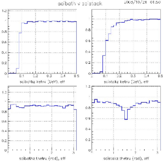
Figure A.3: Reconstructible events versus true angle and energy in Scistack versus Scibath. Upper left corresponds to true kinetic energy of Scibath event; upper right to true kinetic energy of Scistack protons. Bottom left and right are true angle for Scibath and Scistack respectively.

A.4 Conclusions

While the Scistack detector technology is proven experimentally, it is not suitable for FINeSSE’s $\Delta s$ measurements. Scibath, by contrast, has the ability to reconstruct even low $Q^{2}$ events, crucial for this analysis.

Appendix B FESS Project Definition Report
The FINeSSE Detector

Bibliography

- [1]
- [2] J. Ashman et al. [European Muon Collaboration], Phys. Lett. B 206, 364 (1988).
- [3] G. M. Fuller and B. S. Meyer, Neutrino Capture and Supernova Nucleosynthesis, Astrophys. J453, 792 (1995).
- [4] A. A. Aguilar-Arevalo et al., “The MiniBooNE Run Plan”, October 2003.
- [5] ”Report to the Fermilab Director by the Proton Committee”, October, 2003. http://www.fnal.gov/orgs/fermilab_users_org/docs_03_04/ProtonReport.pdf.
- [6] B. W. Filippone and X. D. Ji, Adv. Nucl. Phys. 26, 1 (2001) [arXiv:hep-ph/0101224].
- [7] S. J. Brodsky et al., Phys. Lett. B206, 309 (1988).
- [8] S. D. Bass, hep-ph/0311174; S. D. Bass and A. W. Thomas, hep-ph/9310306.
- [9] S. L. Adler, Phys. Rev. 177, 2426 (1969); J. S. Bell and R. Jackiw, Nuovo Cimento 60A, 47 (1969).
- [10] S.-L. Zhu et al., Phys. Rev. D66 034021 (2002).
- [11] A. O. Bazarko et al., Z. Phys. C65, 189 (1995), hep-ex/9406007; M. Goncharov et al., Phys. Rev. D 64, 112006 (2001), hep-ex/0102049.
- [12] R. D. McKeown and M. J. Ramsey-Musolf, hep-ph/0203011; R. Hasty et al., Science 290, 2117 (2000); T. M. Ito et al., nucl-ex/0310001.
- [13] K. A. Anoil et al., Phys. Lett. B509, 211 (2001).
- [14] JLab experiments E99-115 and E00-114.
- [15] http://www.kph.uni-mainz.de/A4/Welcome.html.
- [16] http://www.npl.uiuc.edu/exp/G0/.
- [17] S. Pate, hep-ex/0310052.
- [18] D. Adams et al., Phys. Rev. D56, 5330 (1997).
- [19] M. Glück et al., Phys. Rev. D63 094005 (2001).
- [20] A. Airapetian et al., hep-ex/0307064 v2.
- [21] L. A. Ahrens et al., Phys. Rev. D35, 785 (1987).
- [22] G. Garvey et al., Phys. Rev. C48, 761 (1993).
- [23] W. M. Alberico et al., Nucl. Phys. A651, 277 (1999).
- [24] J.R. Ellis, A. Ferstl and K.A. Olive, “Theoretical aspects of dark matter detection,” hep-ph/0106148..
- [25] K. A. Olive, arXiv:hep-ph/0308035.
- [26] See, for example: V. A. Bednyakov, arXiv:hep-ph/0310041.
- [27] G. Garvey et al., Phys. Lett. B289, 249 (1992); Phys. Rev. C48, 1919 (1993).
- [28] V. Bernard et al., J. Phys. G: Nucl. Part. Phys. 28 R1 (2002), hep-ph/107088 .
- [29] R. M. Barnett, Phys. Rev. D14, 2990 (1976).
- [30] C. J. Horowitz et al., Phys. Rev. C 48, 3078 (1993).
- [31] H. Kim et al., Phys. Rev. C 51, 2739 (1995).
- [32] M. B. Barbaro et al., Phys. Rev. C54, 1954 (1996).
- [33] W. M Alberico et al., hep-ph/0311053.
- [34] C. Maieron and W. M Alberico, internal memo (2003).
- [35] B. I. S. van der Ventel and J. Piekarewicz, hep-ph/0310047 (2003).
- [36] A. Aguilar et al., Phys. Rev. D64, 112007 (2001).
- [37] B. Armbruster et al., Phys. Rev. D65, 112001 (2002).
- [38] B. Achkar et al., Nucl. Phys. B434, 503 (1995).
- [39] E. D. Church, K. Eitel, G. B Mills, and M. Steidl, Phys. Rev. D66, 013001 (2002).
- [40] For discussion see: S. Hannestad, JCAP 0305:004 (2003), astro-ph/0303076; V. Barger et al., Phys. Lett. B566, 8 (2003), hep-ph/0305075; K. Abazajian, Astropart. Phys. 19, 303 (2003), astro-ph/0205238.
- [41] Representative examples: B. H. J. McKellar et al., hep-ph/0106121; R. N. Mohapatra, Phys. Rev. D64, 091301 (2001), hep-ph/0107264; A. Ioannisian and J. W. F. Valle, Phys. Rev. D63, 073002 (2001); E. Ma, G. Rajasekaran, and U. Sarkar, Phys. Lett. B495, 363 (2000), hep-ph/0006340; Z. Berezhiani and R. Mohapatra, Phys. Rev. D52, 6607 (1995).
- [42] M. Sorel, J. Conrad, and M. Shaevitz, hep-ph/0305255.
- [43] R. D. Hoffman, S. E. Woosley, and Y.-Z. Qian, Astrophys. J482, 951 (1996); G. C. McLaughlin and G. M. Fuller, Astrophys. J472, 440 (1996); B. S. Meyer and J. S. Brown, Astrophys. J. Suppl, 112 199 (1997).
- [44] For a nice explanation of the -process, see M. Patel and G. M. Fuller, hep-ph/0003034.
- [45] S. Rosswog et al., Astron. Astrophys. 341, 499 (1999).
- [46] G. C. McLaughlin et al., Phys. Rev. C59 2873 (1999).
- [47] L. Wolfenstein, Phys. Rev. D17, 2369 (1978); D20, 2634 (1979); S. P. Mikheyev and A. Yu. Smirnov, Yad. Fiz. 42, 1441 (1985) [Sov. J. Nucl. Phys. 42, 913 (1986)]; Nuovo Cimento 9C, 17 (1986).
- [48] A. Choi, private communication.
- [49] http://wwwasd.web.cern.ch/wwwasd/geant4/G4UsersDocuments/Overview/html; M. Sorel, “The GEANT4-based beam Monte Carlo for MiniBooNE”, MiniBooNE technical note, October 2003.
- [50] J. R. Sanford and C. L. Wang, BNL AGS internal reports # BNL11299, BNL11479 (1967); J. Monroe, “A Sanford–Wang Global Fit to Pion Production Data in the Momentum and Production Angle Range of Interest for the MiniBooNE experiment”, MiniBooNE memorandum, September 2003.
- [51] I. Chemakin et al., Phys. Rev. C65, 024904 (2002), nucl-ex/0108007.
- [52] HARP collaboration, Status Report to SPSC, CERN-SPSC/2003-027, August 2003.
- [53] M. Sorel, “Error on the MiniBooNE neutrino flux arising from finite HARP statistics”, MiniBooNE memorandum, August 2002.
- [54] D. Casper, Nucl. Phys. Proc. Suppl. 112, 161 (2002).
- [55] P. Border et al., Nucl. Instr. Meth. A463, 194 (2001).
- [56] Saint-Gobain Crystals and Detectors, Newbury, OH 44065-9677.
- [57] Kuraray Co., Ltd. New York, NY 10166.
- [58] Keith Ruddick, U. Minnesota, private communication.
- [59] M. Doucet, J. P. Fabre, G. Gregoire, J. Panman and P. Zuchelli, Nucl. Instr. Meth. A453, 545 (2000).
- [60] B. Chaudhury, NuMI-L-306, Fermilab.
- [61] Y. Hayato, “K2K Near Detector Upgrade”, NuInt02 workshop proceedings, to appear in Nucl. Proc. Suppl. (2004).
- [62] http://www.iucf.indiana.edu/RERP.
- [63] MINOS collaboration, “The MINOS Technical Design Report”, NuMI-L-337.
- [64] C.E. Allgower et al., Nucl. Instrum. Meth. A 499, 740 (2003).
- [65] I. Stancu et al. [MiniBooNE collaboration], “The Miniboone Detector Technical Design Report,” FERMILAB-TM-2207.
- [66] Alan Bross, private communication.
- [67] Project Definition Report, “FINeSSE Detector”, FESS/Engineering Project No. 6-7-59.
- [68] R. Brun, R. Hagelberg, M. Hansroul and J. C. Lassalle, “Geant: Simulation Program For Particle Physics Experiments. User Guide And Reference Manual,” CERN-DD-78-2-REV.
- [69] P. V. C. Hough, “Machine Analysis of Bubble Chamber Pictures”, International Conference on High Energy Accelerators and Instrumentation, CERN, (1959).
- [70] P. Kasper, J. Link, P. Martin. “MiniBooNE Target Station Shielding Assessment”. http://www-boone.fnal.gov/safety_docs/SAD/shielding_phIII.doc.
- [71] H. Moraal et al., Prepared for 27th International Cosmic Ray Conference (ICRC 2001), Hamburg, Germany, 7-15 Aug 2001.
- [72] J. M. Clem Prepared for 26th International Cosmic Ray Conference (ICRC 99), Salt Lake City, Utah, 17-25 Aug 1999.
- [73] http://www.eljentechnology.com/ej-321.htm
- [74] Minikata et al., hep-ph/0211111.
- [75] MiniBooNE Expression of Interest, turned into the PAC for the Dec. 12, 2003 Meeting.
- [76] P. Lipari, Nucl. Phys. Proc. Suppl. 112, 274 (2002).
- [77] A. Suzuki et al., Nucl. Instr. Meth. A453, 165 (2000); T. Ishii et al., Nucl. Instr. Meth. A482, 244 (2002).
- [78] T. Ishida, Nucl. Proc. Suppl. 112, 132 (2002); C. Mauger, Nucl. Phys. Proc. Suppl. 112, 146 (2002); C. W. Walter, Nucl. Phys. Proc. Suppl. 112, 140 (2002).
- [79] D. Rein and L. M. Sehgal, Annals Phys 133, 79 (1981).
- [80] D. Casper, Nucl. Phys. Proc. Suppl. 112, 161 (2002); H. Gallagher, Nucl. Proc. Suppl. 112, 188 (2002).
- [81] E. Hawker, “Single Pion Production in Low Energy Neutrino-Carbon Interactions”, NuInt02 workshop proceedings, to appear in Nucl. Proc. Suppl. (2004).
- [82] P. Vilain et al., Phys. Lett. 313B, 267 (1993).
- [83] H. Faissner et al., Phys. Lett. 125B, 230 (1983).
- [84] E. A. Paschos and A. V. Kartavtsev, hep-ph/0309148; J. Marteau et al., hep-ph/9906449.
- [85] D. Rein and L. M. Sehgal, Nucl. Phys. B223, 29 (1983).
- [86] Y. Hayato, “K2K Near Detector Upgrade”, NuInt02 workshop proceedings, to appear in Nucl. Proc. Suppl. (2004).
- [87] W. A. Mann et al., Phys. Rev. D34, 2545 (1986).
- [88] R. E. Shrock, Phys. Rev. D12, 2049 (1975); A. A. Amer, Phys. Rev. D18, 2290 (1978).
- [89] M. Frank, “Neutrino magnetic moments in the left-right supersymmetric model,” Phys. Rev. D 60, 093005 (1999).
- [90] G. C. McLaughlin and J. N. Ng, “Astrophysical implications of the induced neutrino magnetic moment from large extra dimensions,” Phys. Lett. B 470, 157 (1999) [hep-ph/9909558].
- [91] M. Fukugita and S. Yazaki, “Reexamination of astrophysical and cosmological constraints on the magnetic moment of neutrinos,” Phys. Rev. D 36, 3817 (1987).
- [92] J. M. Lattimer and J. Cooperstein, “Limits on the neutrino magnetic moment from supernova 1987A,” Phys. Rev. Lett. 61, 23 (1988).
- [93] R. Barbieri and R. N. Mohapatra, “Limit on the magnetic moment of the neutrino from supernova 1987A observations,” Phys. Rev. Lett. 61, 27 (1988).
- [94] L. B. Auerbach et al. [LSND Collaboration], “Measurement of electron-neutrino electron elastic scattering,” Phys. Rev. D 63, 112001 (2001) [hep-ex/0101039].
- [95] J. F. Beacom and P. Vogel, “Neutrino magnetic moments, flavor mixing, and the superKamiokande solar data,” Phys. Rev. Lett. 83, 5222 (1999) [hep-ph/9907383].
- [96] A. I. Derbin, A. V. Chernyi, L. A. Popeko, V. N. Muratova, G. A. Shishkina and S. I. Bakhlanov, “Experiment on anti-neutrino scattering by electrons at a reactor of the Rovno nuclear power plant,” JETP Lett. 57, 768 (1993) [Pisma Zh. Eksp. Teor. Fiz. 57, 755 (1993)].
- [97] A. V. Derbin, “Restriction on the magnetic dipole moment of reactor neutrinos,” Phys. Atom. Nucl. 57, 222 (1994) [Yad. Fiz. 57, 236 (1994)].
- [98] R. Schwienhorst et al. [DONUT Collaboration], “A new upper limit for the tau-neutrino magnetic moment,” Phys. Lett. B 513, 23 (2001) [hep-ex/0102026].
- [99] J. Beacom and B. T. Fleming, in preparation.