Data from decays in DELPHI have been searched for
with the
decaying to
and ,
or . These events are used to
measure the CKM matrix element and the form factor slope, :
corresponding to a branching fraction:
.
Combining these and previous DELPHI measurements gives:
and
.
Using , yields:
The -quark semileptonic branching fraction into a emitted
from higher mass charmed excited states has also been measured to be:
.
(Accepted by Eur. Phys. J.)
J.Abdallah,
P.Abreu,
W.Adam,
P.Adzic,
T.Albrecht,
T.Alderweireld,
R.Alemany-Fernandez,
T.Allmendinger,
P.P.Allport,
U.Amaldi,
N.Amapane,
S.Amato,
E.Anashkin,
A.Andreazza,
S.Andringa,
N.Anjos,
P.Antilogus,
W-D.Apel,
Y.Arnoud,
S.Ask,
B.Asman,
J.E.Augustin,
A.Augustinus,
P.Baillon,
A.Ballestrero,
P.Bambade,
R.Barbier,
D.Bardin,
G.Barker,
A.Baroncelli,
M.Battaglia,
M.Baubillier,
K-H.Becks,
M.Begalli,
A.Behrmann,
E.Ben-Haim,
N.Benekos,
A.Benvenuti,
C.Berat,
M.Berggren,
L.Berntzon,
D.Bertrand,
M.Besancon,
N.Besson,
D.Bloch,
M.Blom,
M.Bluj,
M.Bonesini,
M.Boonekamp,
P.S.L.Booth,
G.Borisov,
O.Botner,
B.Bouquet,
T.J.V.Bowcock,
I.Boyko,
M.Bracko,
R.Brenner,
E.Brodet,
P.Bruckman,
J.M.Brunet,
L.Bugge,
P.Buschmann,
M.Calvi,
T.Camporesi,
V.Canale,
F.Carena,
N.Castro,
F.Cavallo,
M.Chapkin,
Ph.Charpentier,
P.Checchia,
R.Chierici,
P.Chliapnikov,
J.Chudoba,
S.U.Chung,
K.Cieslik,
P.Collins,
R.Contri,
G.Cosme,
F.Cossutti,
M.J.Costa,
D.Crennell,
J.Cuevas,
J.D’Hondt,
J.Dalmau,
T.da Silva,
W.Da Silva,
G.Della Ricca,
A.De Angelis,
W.De Boer,
C.De Clercq,
B.De Lotto,
N.De Maria,
A.De Min,
L.de Paula,
L.Di Ciaccio,
A.Di Simone,
K.Doroba,
J.Drees,
M.Dris,
G.Eigen,
T.Ekelof,
M.Ellert,
M.Elsing,
M.C.Espirito Santo,
G.Fanourakis,
D.Fassouliotis,
M.Feindt,
J.Fernandez,
A.Ferrer,
F.Ferro,
U.Flagmeyer,
H.Foeth,
E.Fokitis,
F.Fulda-Quenzer,
J.Fuster,
M.Gandelman,
C.Garcia,
Ph.Gavillet,
E.Gazis,
R.Gokieli,
B.Golob,
G.Gomez-Ceballos,
P.Goncalves,
E.Graziani,
G.Grosdidier,
K.Grzelak,
J.Guy,
C.Haag,
A.Hallgren,
K.Hamacher,
K.Hamilton,
S.Haug,
F.Hauler,
V.Hedberg,
M.Hennecke,
H.Herr,
J.Hoffman,
S-O.Holmgren,
P.J.Holt,
M.A.Houlden,
K.Hultqvist,
J.N.Jackson,
G.Jarlskog,
P.Jarry,
D.Jeans,
E.K.Johansson,
P.D.Johansson,
P.Jonsson,
C.Joram,
L.Jungermann,
F.Kapusta,
S.Katsanevas,
E.Katsoufis,
G.Kernel,
B.P.Kersevan,
U.Kerzel,
A.Kiiskinen,
B.T.King,
N.J.Kjaer,
P.Kluit,
P.Kokkinias,
C.Kourkoumelis,
O.Kouznetsov,
Z.Krumstein,
M.Kucharczyk,
J.Lamsa,
G.Leder,
F.Ledroit,
L.Leinonen,
R.Leitner,
J.Lemonne,
V.Lepeltier,
T.Lesiak,
W.Liebig,
D.Liko,
A.Lipniacka,
J.H.Lopes,
J.M.Lopez,
D.Loukas,
P.Lutz,
L.Lyons,
J.MacNaughton,
A.Malek,
S.Maltezos,
F.Mandl,
J.Marco,
R.Marco,
B.Marechal,
M.Margoni,
J-C.Marin,
C.Mariotti,
A.Markou,
C.Martinez-Rivero,
J.Masik,
N.Mastroyiannopoulos,
F.Matorras,
C.Matteuzzi,
F.Mazzucato,
M.Mazzucato,
R.Mc Nulty,
C.Meroni,
E.Migliore,
W.Mitaroff,
U.Mjoernmark,
T.Moa,
M.Moch,
K.Moenig,
R.Monge,
J.Montenegro,
D.Moraes,
S.Moreno,
P.Morettini,
U.Mueller,
K.Muenich,
M.Mulders,
L.Mundim,
W.Murray,
B.Muryn,
G.Myatt,
T.Myklebust,
M.Nassiakou,
F.Navarria,
K.Nawrocki,
R.Nicolaidou,
M.Nikolenko,
A.Oblakowska-Mucha,
V.Obraztsov,
A.Olshevski,
A.Onofre,
R.Orava,
K.Osterberg,
A.Ouraou,
A.Oyanguren,
M.Paganoni,
S.Paiano,
J.P.Palacios,
H.Palka,
Th.D.Papadopoulou,
L.Pape,
C.Parkes,
F.Parodi,
U.Parzefall,
A.Passeri,
O.Passon,
L.Peralta,
V.Perepelitsa,
A.Perrotta,
A.Petrolini,
J.Piedra,
L.Pieri,
F.Pierre,
M.Pimenta,
E.Piotto,
T.Podobnik,
V.Poireau,
M.E.Pol,
G.Polok,
P.Poropat,
V.Pozdniakov,
N.Pukhaeva,
A.Pullia,
J.Rames,
L.Ramler,
A.Read,
P.Rebecchi,
J.Rehn,
D.Reid,
R.Reinhardt,
P.Renton,
F.Richard,
J.Ridky,
M.Rivero,
D.Rodriguez,
A.Romero,
P.Ronchese,
P.Roudeau,
T.Rovelli,
V.Ruhlmann-Kleider,
D.Ryabtchikov,
A.Sadovsky,
L.Salmi,
J.Salt,
A.Savoy-Navarro,
U.Schwickerath,
A.Segar,
R.Sekulin,
M.Siebel,
A.Sisakian,
G.Smadja,
O.Smirnova,
A.Sokolov,
A.Sopczak,
R.Sosnowski,
T.Spassov,
M.Stanitzki,
A.Stocchi,
J.Strauss,
B.Stugu,
M.Szczekowski,
M.Szeptycka,
T.Szumlak,
T.Tabarelli,
A.C.Taffard,
F.Tegenfeldt,
J.Timmermans,
L.Tkatchev,
M.Tobin,
S.Todorovova,
B.Tome,
A.Tonazzo,
P.Tortosa,
P.Travnicek,
D.Treille,
G.Tristram,
M.Trochimczuk,
C.Troncon,
M-L.Turluer,
I.A.Tyapkin,
P.Tyapkin,
S.Tzamarias,
V.Uvarov,
G.Valenti,
P.Van Dam,
J.Van Eldik,
A.Van Lysebetten,
N.van Remortel,
I.Van Vulpen,
G.Vegni,
F.Veloso,
W.Venus,
P.Verdier,
V.Verzi,
D.Vilanova,
L.Vitale,
V.Vrba,
H.Wahlen,
A.J.Washbrook,
C.Weiser,
D.Wicke,
J.Wickens,
G.Wilkinson,
M.Winter,
M.Witek,
O.Yushchenko,
A.Zalewska,
P.Zalewski,
D.Zavrtanik,
V.Zhuravlov,
N.I.Zimin,
A.Zintchenko,
M.Zupan11footnotetext: Department of Physics and Astronomy, Iowa State
University, Ames IA 50011-3160, USA
22footnotetext: Physics Department, Universiteit Antwerpen,
Universiteitsplein 1, B-2610 Antwerpen, Belgium
and IIHE, ULB-VUB,
Pleinlaan 2, B-1050 Brussels, Belgium
and Faculté des Sciences,
Univ. de l’Etat Mons, Av. Maistriau 19, B-7000 Mons, Belgium
33footnotetext: Physics Laboratory, University of Athens, Solonos Str.
104, GR-10680 Athens, Greece
44footnotetext: Department of Physics, University of Bergen,
Allégaten 55, NO-5007 Bergen, Norway
55footnotetext: Dipartimento di Fisica, Università di Bologna and INFN,
Via Irnerio 46, IT-40126 Bologna, Italy
66footnotetext: Centro Brasileiro de Pesquisas Físicas, rua Xavier Sigaud 150,
BR-22290 Rio de Janeiro, Brazil
and Depto. de Física, Pont. Univ. Católica,
C.P. 38071 BR-22453 Rio de Janeiro, Brazil
and Inst. de Física, Univ. Estadual do Rio de Janeiro,
rua São Francisco Xavier 524, Rio de Janeiro, Brazil
77footnotetext: Collège de France, Lab. de Physique Corpusculaire, IN2P3-CNRS,
FR-75231 Paris Cedex 05, France
88footnotetext: CERN, CH-1211 Geneva 23, Switzerland
99footnotetext: Institut de Recherches Subatomiques, IN2P3 - CNRS/ULP - BP20,
FR-67037 Strasbourg Cedex, France
1010footnotetext: Now at DESY-Zeuthen, Platanenallee 6, D-15735 Zeuthen, Germany
1111footnotetext: Institute of Nuclear Physics, N.C.S.R. Demokritos,
P.O. Box 60228, GR-15310 Athens, Greece
1212footnotetext: FZU, Inst. of Phys. of the C.A.S. High Energy Physics Division,
Na Slovance 2, CZ-180 40, Praha 8, Czech Republic
1313footnotetext: Dipartimento di Fisica, Università di Genova and INFN,
Via Dodecaneso 33, IT-16146 Genova, Italy
1414footnotetext: Institut des Sciences Nucléaires, IN2P3-CNRS, Université
de Grenoble 1, FR-38026 Grenoble Cedex, France
1515footnotetext: Helsinki Institute of Physics, P.O. Box 64,
FIN-00014 University of Helsinki, Finland
1616footnotetext: Joint Institute for Nuclear Research, Dubna, Head Post
Office, P.O. Box 79, RU-101 000 Moscow, Russian Federation
1717footnotetext: Institut für Experimentelle Kernphysik,
Universität Karlsruhe, Postfach 6980, DE-76128 Karlsruhe,
Germany
1818footnotetext: Institute of Nuclear Physics,Ul. Kawiory 26a,
PL-30055 Krakow, Poland
1919footnotetext: Faculty of Physics and Nuclear Techniques, University of Mining
and Metallurgy, PL-30055 Krakow, Poland
2020footnotetext: Université de Paris-Sud, Lab. de l’Accélérateur
Linéaire, IN2P3-CNRS, Bât. 200, FR-91405 Orsay Cedex, France
2121footnotetext: School of Physics and Chemistry, University of Lancaster,
Lancaster LA1 4YB, UK
2222footnotetext: LIP, IST, FCUL - Av. Elias Garcia, 14-,
PT-1000 Lisboa Codex, Portugal
2323footnotetext: Department of Physics, University of Liverpool, P.O.
Box 147, Liverpool L69 3BX, UK
2424footnotetext: Dept. of Physics and Astronomy, Kelvin Building,
University of Glasgow, Glasgow G12 8QQ
2525footnotetext: LPNHE, IN2P3-CNRS, Univ. Paris VI et VII, Tour 33 (RdC),
4 place Jussieu, FR-75252 Paris Cedex 05, France
2626footnotetext: Department of Physics, University of Lund,
Sölvegatan 14, SE-223 63 Lund, Sweden
2727footnotetext: Université Claude Bernard de Lyon, IPNL, IN2P3-CNRS,
FR-69622 Villeurbanne Cedex, France
2828footnotetext: Dipartimento di Fisica, Università di Milano and INFN-MILANO,
Via Celoria 16, IT-20133 Milan, Italy
2929footnotetext: Dipartimento di Fisica, Univ. di Milano-Bicocca and
INFN-MILANO, Piazza della Scienza 2, IT-20126 Milan, Italy
3030footnotetext: IPNP of MFF, Charles Univ., Areal MFF,
V Holesovickach 2, CZ-180 00, Praha 8, Czech Republic
3131footnotetext: NIKHEF, Postbus 41882, NL-1009 DB
Amsterdam, The Netherlands
3232footnotetext: National Technical University, Physics Department,
Zografou Campus, GR-15773 Athens, Greece
3333footnotetext: Physics Department, University of Oslo, Blindern,
NO-0316 Oslo, Norway
3434footnotetext: Dpto. Fisica, Univ. Oviedo, Avda. Calvo Sotelo
s/n, ES-33007 Oviedo, Spain
3535footnotetext: Department of Physics, University of Oxford,
Keble Road, Oxford OX1 3RH, UK
3636footnotetext: Dipartimento di Fisica, Università di Padova and
INFN, Via Marzolo 8, IT-35131 Padua, Italy
3737footnotetext: Rutherford Appleton Laboratory, Chilton, Didcot
OX11 OQX, UK
3838footnotetext: Dipartimento di Fisica, Università di Roma II and
INFN, Tor Vergata, IT-00173 Rome, Italy
3939footnotetext: Dipartimento di Fisica, Università di Roma III and
INFN, Via della Vasca Navale 84, IT-00146 Rome, Italy
4040footnotetext: DAPNIA/Service de Physique des Particules,
CEA-Saclay, FR-91191 Gif-sur-Yvette Cedex, France
4141footnotetext: Instituto de Fisica de Cantabria (CSIC-UC), Avda.
los Castros s/n, ES-39006 Santander, Spain
4242footnotetext: Inst. for High Energy Physics, Serpukov
P.O. Box 35, Protvino, (Moscow Region), Russian Federation
4343footnotetext: J. Stefan Institute, Jamova 39, SI-1000 Ljubljana, Slovenia
and Laboratory for Astroparticle Physics,
Nova Gorica Polytechnic, Kostanjeviska 16a, SI-5000 Nova Gorica, Slovenia,
and Department of Physics, University of Ljubljana,
SI-1000 Ljubljana, Slovenia
4444footnotetext: Fysikum, Stockholm University,
Box 6730, SE-113 85 Stockholm, Sweden
4545footnotetext: Dipartimento di Fisica Sperimentale, Università di
Torino and INFN, Via P. Giuria 1, IT-10125 Turin, Italy
4646footnotetext: INFN,Sezione di Torino, and Dipartimento di Fisica Teorica,
Università di Torino, Via P. Giuria 1,
IT-10125 Turin, Italy
4747footnotetext: Dipartimento di Fisica, Università di Trieste and
INFN, Via A. Valerio 2, IT-34127 Trieste, Italy
and Istituto di Fisica, Università di Udine,
IT-33100 Udine, Italy
4848footnotetext: Univ. Federal do Rio de Janeiro, C.P. 68528
Cidade Univ., Ilha do Fundão
BR-21945-970 Rio de Janeiro, Brazil
4949footnotetext: Department of Radiation Sciences, University of
Uppsala, P.O. Box 535, SE-751 21 Uppsala, Sweden
5050footnotetext: IFIC, Valencia-CSIC, and D.F.A.M.N., U. de Valencia,
Avda. Dr. Moliner 50, ES-46100 Burjassot (Valencia), Spain
5151footnotetext: Institut für Hochenergiephysik, Österr. Akad.
d. Wissensch., Nikolsdorfergasse 18, AT-1050 Vienna, Austria
5252footnotetext: Inst. Nuclear Studies and University of Warsaw, Ul.
Hoza 69, PL-00681 Warsaw, Poland
5353footnotetext: Fachbereich Physik, University of Wuppertal, Postfach
100 127, DE-42097 Wuppertal, Germany
1 Introduction
The Cabibbo, Kobayashi and Maskawa (CKM) matrix
element is a parameter of the Standard Model and its value
needs to be fixed by experiments. This parameter determines the decay rate of
-hadrons because governs the other possible
charged weak decay of -quarks and contributes only 1-2 to the total
decay rate. The value of cannot be measured directly and there are two
decay processes for which theoretical uncertainties are expected to be
under control [1]: the inclusive semileptonic decay of
-hadrons corresponding
to the transition and the
exclusive decay channel
.
The latter is used in the following analysis, the 111 Throughout this paper charge-conjugate states are
implicitly included.
is reconstructed
through its decay to and the meson is isolated
using three decay channels: ,
and .
This study benefits from the reprocessing of DELPHI data taken
between 1992 and 1995 through improved versions of the event reconstruction
algorithms. As a consequence, the number of signal events has increased
by more than a factor two over those reported in
[2] using the same decay final states.
An additional decay channel of the ()
has been analysed which provides
another factor of two increase. There are also improvements
on the mass
and -meson energy reconstruction.
The signal is now
narrower which gives a better isolation of the signal over
the combinatorial background. As the main source of
experimental systematic uncertainty originates from the contribution
of mesons emitted in the decay of excited charmed states
produced in -hadron semileptonic decays, additional observables have been
defined to control the level of this contamination in a better way.
The evaluation of the remaining contamination from the
double charm cascade decays
()
benefits from recent measurements of their rates.
2 Measurement of from the decay
The value of is extracted by studying
the decay partial width for the process
as a function of the recoil kinematics
of the meson [1]. The decay rate is parameterized as
a function
of the variable , defined as the product of the four-velocities of the
and mesons.
This variable is related to the square of
the four-momentum transfer from the to the
system, , by:
(1)
and its value ranges from , when the is produced at rest in the
rest
frame, to about . Using the Heavy Quark Effective Theory
(HQET)[3],
the
differential partial width
for this
decay is given by:
(2)
where contains kinematic factors:
(3)
with
and is a hadronic form factor.
Although the shape of the
form factor, , is not known, its magnitude
at zero recoil, corresponding to , can be estimated using HQET.
It is convenient to express in terms
of the axial form factor
and of the reduced helicity form factors
and :
(4)
The reduced helicity form factors are themselves expressed in terms of the
ratios between the other HQET form factors
() and :
(5)
(6)
with
(7)
Values for and have been measured by CLEO
[4] using different models.
The unknown function is approximated with an expansion
around [5]:
(8)
where is the slope parameter at zero recoil and
.
An alternative parametrization, obtained earlier, can be found in
[6].
In the heavy quark limit (),
coincides with the Isgur-Wise function [7, 8] which is
normalized to unity at the point of zero recoil.
Corrections to have been calculated to take into account
the effects of finite quark masses and QCD corrections
They yield [9].
Experiments determine the product
by fitting this quantity and the slope ,
using the expression (2), convoluted with the experimental
resolution on the variable.
Since the phase space factor tends to zero
as , the decay rate vanishes
in this limit and the
accuracy of the extrapolation relies on achieving a reasonably
constant reconstruction efficiency in the region close to .
Results of the following analysis are expressed in terms of the
variable.
3 The DELPHI detector
The DELPHI detector and its performance have been described in detail
elsewhere [10].
The tracking system consisted of the
Vertex Detector (VD), the Inner Detector (ID), the Time Projection Chamber
(TPC) and the Outer Detector (OD) in the barrel region while the Forward
Chambers (FCA, FCB) covered the end-cap regions. The
average momentum resolution for high momentum charged particles traversing
the DELPHI magnetic field of T was
in
the polar angle region between and .
The VD surrounded the beam pipe and consisted of three concentric layers of
silicon micro-strip detectors at radii , and cm.
Until 1994 the VD layers were single-sided and provided only information
in the plane222 In the DELPHI coordinate system, is
along the electron beam direction, and R are the azimuthal angle and
radius
in the plane, and is the polar angle with respect to
the axis.. In 1994 the innermost and outermost layers were
replaced by double-sided silicon micro-strip modules
providing
both and measurements.
The ID was placed outside the VD and consisted of a jet chamber
providing information, and a trigger chamber providing a measurement
of the coordinate.
In 1995 a new ID was installed with
a longer jet chamber and straw tubes replacing the trigger chambers.
The VD and ID were surrounded by the TPC, the main
DELPHI tracking device. The TPC provided up to 16 space points per particle
trajectory between radii of and cm. The OD consisted of 5
layers of drift tubes and complemented the TPC by improving the momentum
resolution of charged particles.
Hadrons were identified using the specific ionization () in the TPC
and the Cherenkov radiation in the barrel Ring Imaging CHerenkov detector
(RICH) placed between the TPC and OD detectors.
The muon identification relied mainly on the muon chambers, a set of drift
chambers giving three-dimensional information located at the periphery of
DELPHI after approximately m of iron.
Electron identification relied mainly on the electromagnetic calorimeter
in the barrel region (High density Projection Chamber, HPC) which was a
sampling device having a relative energy resolution of for
electrons with momentum, and a spatial resolution
of mm in .
4 Hadronic Event Selection and Simulation
Hadronic decays collected by DELPHI between 1992 and 1995 have
been analysed. Each event was divided into two hemispheres by a plane
orthogonal to the thrust axis. To ensure that the event was well contained
inside the fiducial volume of the detector, the cosine of the
polar angle of the thrust
axis of the event had to lie between -0.95 and +0.95.
Charged and neutral particles were
clustered into jets by using the LUCLUS algorithm [11] with
the resolution
parameter .
About 3.4 million events were selected from the full LEP1 data sets.
The JETSET 7.3 Parton Shower program [11] was used to generate
hadronic decays, which were followed through the detailed detector
simulation DELSIM [10] and finally processed by the same
analysis chain as the real data. A sample of about nine million
events was used. To increase the statistical
significance of the simulation, an additional sample of about 3.6 million
events was analysed, equivalent to about
17 million hadronic decays. Statistics for the hadronic samples
are given in Table 1.
Year
Real data
Simulated
Simulated
1992+1993
1355805
3916050
1096199
1994+1995
2012921
5012881
2495335
Total
3368726
8928931
3591534
Table 1: Analysed number of events. In 1992 and 1993
only two-dimensional vertex reconstruction was available.
5 Selection of events for analysis
Events corresponding to candidates for the decay
are selected
by requiring the presence of an identified lepton and of a
candidate in the same event hemisphere
which is defined by the direction of the jet containing the lepton.
are measured using the decays to . mesons
are reconstructed using their decays into ,
and .
To reduce the contribution
from decays into light flavours,
the standard DELPHI event -tagging variable [10]
is used to enhance the sample
in
decays. The -tagging variable is
essentially
the probability that
the analysed
event originates from light quarks and is required to be less than 0.5
for decays and less than 0.1 for the
decay.
In addition, the mass of the system is restricted
to the range between 2.5 and 5.5 .
5.1 Lepton identification
Muons and electrons with momentum larger than 2 and at least one
associated hit in the VD are selected.
Muons are identified using standard algorithms [10] based on the matching
of the track reconstructed in the tracking system to the
track elements provided by the barrel and forward
muon chambers. Loose selection criteria
are applied and the efficiency is for
probability of hadron misidentification.
Electrons are identified using a neural
network algorithm
providing about 75 efficiency within the calorimeter
acceptance. The probability for a hadron to fake an electron was about 1.
Electrons from photon conversions are mainly produced in the outer ID wall
and in the inner TPC frame. About 80 of them were removed, with negligible
loss of signal, by reconstructing
the conversion vertex.
5.2 Isolation of the decay channel
The kaon candidate corresponds to a particle
with the same charge as the lepton,
with a momentum
larger than 1 and not identified as a pion by the standard algorithms
[10]
which combine information provided by the ionization deposited
in the gas volume of the TPC and by the RICH detectors.
The pion candidate must have a charge opposite to the kaon and a
momentum larger than 0.5 . The pion and kaon candidates must both
have at least one
associated VD hit in
and be situated in the same
event hemisphere as
the jet containing the lepton.
The two tracks must intersect in space
to form a decay vertex candidate
and those with a probability lower
than 10-3 are rejected. systems with a mass
between 1.81 and 1.92 and with a momentum larger than
6 are selected as signal candidates. Resolutions on the reconstructed
mass measured on real and simulated events are given in
Table 2. The selected mass window for the signal corresponds
to about .
A track is then reconstructed using the parameters of the and
tracks fitted at their common vertex and imposing the condition that
the mass, quoted as in the following,
is 1.8645 [9].
decay channel
92-93 MC
92-93 data
94-95 MC
94-95 data
Table 2: Mass resolution for signals measured on real
and simulated events.
The B decay vertex is obtained from the intersection of
the and the lepton trajectories. This vertex must have
a probability larger than 10-3 and only pairs of
total momentum larger than 10 are kept. The B decay vertex is then
required to be at a minimum distance from the position of the beam
interaction point.
This algebraic distance is evaluated
along the direction of the momentum.
A minimum distance
between the D and B measured decay points,
evaluated along the
momentum, is also required. These conditions
depend on the number of VD hits associated to the tracks.
If the
decay distance is not measured along with the VD, only cuts on decay
distances transverse to the beam direction are applied.
These requirements, which are rather loose, are given in Table 3.
decay channel
B vert. main vert.
D vert.
B vert.
Table 3: Minimum requirements on the decay distance between
the B decay and the main vertices and also between the D and the B decay
vertices. The first
number corresponds to the cut in space whereas the second is the
transverse distance cut, which is applied only when the z coordinate
is not measured. Negative distances corespond to positions behind the beam
interaction point.
The signal is identified by its decay to . Each
particle of charge opposite to the lepton candidate and emitted in the same
event hemisphere as the jet containing the lepton is considered as a
candidate for the .
The track of this particle must form a vertex
with the and the charged lepton trajectories and the vertex fit
probability has to be higher than 10-3. Signals for the cascade decay
correspond to a peak in
the distribution of the mass difference
.
The global efficiencies to select signal events
have been estimated using the simulation
(see Table 4), accounting for
all analysis steps described above, apart from the branching fractions of
the and
of the into the selected decay channels.
decay channel
92-93 MC
94-95 MC
Table 4: Global efficiencies of the analysis chain to reconstruct
and select simulated signal events.
The quoted uncertainties are statistical.
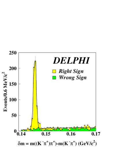
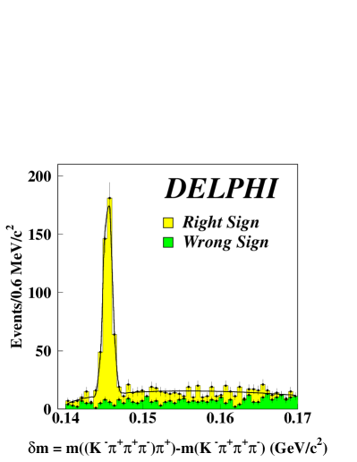
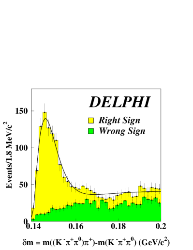
Figure 1: distributions for the
(upper),
(middle)
and (lower) decay channels.
Combinations with the wrong K-lepton charge correlation are superimposed as
darker histograms.
Events registered in 92-93 and 94-95 have not been distinguished.
The curves show the fits to the right-sign distributions described in the
text.
5.3 Isolation of the
decay channel
Similar selection criteria to those which were applied to isolate the
decay channel, are used. Differences
in the algorithm are related to the final state multiplicity.
Each of the three pion candidates must have a
momentum larger than 0.5 and the total charge of the three pion system
has to be opposite to the kaon charge.
At least two, among the four charged particle track candidates for decay
products
must be
associated to at least one VD hit in and be situated in the same
event hemisphere as
the jet containing the lepton.
As the reconstructed signal is narrower,
systems with a mass
between 1.84 and 1.90 are selected.
The measured mass resolutions
are given in Table 2.
Because of the higher combinatorial background, as compared with the
decay channel, cuts
on algebraic distances between the B and the main vertex and between
the D and the B decay vertex
are more
severe than for the previous channel. They are summarized in
Table 3.
The same set of four particles can give two
mass combinations if there is an ambiguity in the definition
of the and candidates. Only one combination is kept
in the analysis by
using criteria which are based on the available particle identification
information provided by the RICH and the TPC
or,
if this information is missing, assuming that the
has the larger momentum.
The same selection criteria, as for the decay
, are applied to
search for a signal.
The global efficiencies to select signal events
have been estimated using the simulation
(see Table 4), accounting for
all analysis steps described above, apart from the branching fractions of
the and
of the into the selected decay channels.
5.4 Isolation of the
decay channel
The same criteria are applied, as in Section 5.2,
to select the and candidates apart from the
cut on the mass which is required now to be between
1.5 and 1.7 . This mass interval corresponds to the
satellite peak position for the decay
when the emitted from the is soft.
An estimate of the 4-vector is obtained by assuming that the
decay is of the type and the , and
masses are used as constraints.
In addition it has been assumed that the is contained in the
plane defined by the and the . When two solutions are
possible, a choice is made according to criteria which have been
defined using simulated events.
The signal is identified by its decay to . Each
particle of charge opposite to the lepton candidate and emitted in the same
event hemisphere as the jet containing the lepton is considered as a
candidate for the .
The track of this particle must form a vertex
with the and the charged lepton trajectories and the vertex fit
probability has to be higher than 10-3. Signals for the cascade decay
correspond to a peak in
the distribution of the mass difference
. The peak is broader than for
cases in which the was completely reconstructed using its
charged decay products.
Cuts on decay distances between the primary, the B and the D vertex
are given in Table 3.
The global efficiencies to select signal events
have been estimated using the simulation
(see Table 4), accounting for
all analysis steps described above, apart from the branching fractions of
the and
of the into the selected decay channels.
The event selection described above does not ensure
that only decaying into the channel are selected.
The simulation predicts that about 67 are of this origin and that there
are also: (18),
(3) where X corresponds to neutrals,
(3) where the is assumed to be a
and
the remaining 10 originates from various other channels.
Apart from the
last contribution, efficiencies have been determined for each individual
channel using the simulation.
Table 4 shows the selection efficiency corresponding to
the weighted average for these channels.
The branching fractions measured for each of these
channels have been used for the real data
(apart from which is assumed to be the same
as in the simulation and equal to 5.6, with an error of 0.6) and a
corresponding effective efficiency has been evaluated.
A correction factor for the remaining 10 of the events of undetermined
origin has been obtained from a fit to the simulation using the
efficiencies of the four identified contributions (see Table
4) and ensuring that the
simulated
is
recovered. This
correction
has been used on real data with a relative uncertainty of ,
corresponding to the statistical error of the fit
on simulated events.
5.5 Selected event candidates
The mass difference distributions corresponding to the variable
obtained
for the three channels, are shown in Figure 1.
The numbers of candidates obtained by fitting
these distributions with a Gaussian
()
or a gamma distribution ()
for the signal, and a smooth distribution
for the combinatorial background333 The distribution selected for the
combinatorial background
is , with and .
are given in Table 5.
Data set
92-93
94-95
193 15
328 16
144 14
243 17
286 24
494 27
Table 5: Number of candidate events selected
in the two data taking periods and for the three decay channels.
5.6 measurement
As explained in Section 2, to measure it is
necessary to study the dependence of the differential
semileptonic decay partial width . For signal events,
corresponding to the semileptonic decay
, the value
of has been obtained from the measurements of the
and four-momenta:
(9)
The 4-momentum is accurately measured, as all decay products
correspond to reconstructed charged particle trajectories.444 For the
decay channel the accuracy is reduced by about 10
because of the missing .
To improve on the determination of the momentum, information from
all measured -decay products is used, including an evaluation of the
missing momentum in the jet containing the lepton and the positions of
the primary and of the secondary vertex, which are used as constraints to
define the direction of the -hadron momentum.
The nominal mass
is also used as a constraint in this fit.
The missing momentum in each jet has been evaluated by comparing the
reconstructed
jet momentum with the expectation obtained by imposing energy-momentum
conservation on the whole event.
Finally, a momentum dependent correction
is applied to the reconstructed -hadron momentum so that it remains,
for simulated signal events,
centred on the generated value.
The smearing of the variable is studied with simulated signal events.
The function
gives the
distribution of the difference between the values of the reconstructed
, , for events
generated with a given value .
Twenty slices in of the same width have been considered. Within
each slice, is parametrized as the sum
of two Gaussian distributions (see Figure 2).
The two central positions of the Gaussians,
their standard deviations and the fraction of events corresponding to the
narrower Gaussian are parametrized with a linear dependence on .
Such parametrizations are obtained independently for two sets of
ten slices. Typical values of these parametrizations correspond to
resolutions of 0.3 and 2 with about 50 of the events
included in the narrower Gaussian. Resolution distributions obtained
for reconstructed with only charged particles and for
the decay channel are compared in
Figure 3.
Figure 2: Fit of the slices for
the 94-95 data taking period, as expected from simulated events.
The simulated central value is quoted above the corresponding slice.
Figure 3: Comparison between the resolution functions obtained
for decay channels with and without a missing particle for the
92-93 and 94-95 data taking periods, as expected from simulated events.
The cuts applied to select the events which require a minimum momentum on
the lepton, the and the system and the cut
on the minimum value for the mass of the system can
possibly introduce
a bias in the distribution. A dependent acceptance
correction, has been evaluated by comparing the
simulated distributions for signal events
before and after applying all analysis cuts.
This correction has been normalized such that it does not change the
number of accepted events for which an overall efficiency has already been
determined.
The corresponding distribution
is given in Figure 4.
It is uniform and does not show evidence for
any significant bias. A linear dependence for the acceptance gives:
(10)
which is compatible with unity within quoted uncertainties.
As the cuts used in the analysis are very similar for all
data samples, the same
dependent acceptance correction has been used for all channels and
data samples.
Figure 4: Stability of the acceptance
as a function of the value of the simulated .
6 The analysis procedure
The purpose of this analysis is to determine the values of the parameters
and introduced in Section
2,
using the measured distribution
of candidate events.
The predicted distribution for the signal is obtained
using the theoretical distribution
corrected by the overall efficiency and the dependent acceptance,
and then convoluted with the expected resolution function
. The distributions for the other event
sources are taken from the simulation or from the real data
for the
combinatorial background.
The distributions are rather similar for the signal and
other event categories because the procedure used to evaluate
from the and 4-momenta overestimates
the real value for background events.
This is because algorithms have been defined for signal events
and thus do not include the additional hadrons emitted in
background sources.
To enhance the separation between the signal and other event sources,
three other variables have been used. As a result, the branching fraction for
production in the decay of higher mass charm
states,
, has
also been measured.
Before describing these quantities,
the different event classes
contributing to the analysis are explained.
6.1 The Event Sample composition
In addition to the signal (), which corresponds to the decay
,
there are six classes of events which contribute to the background:
•
the combinatorial background (B) under the peak;
•
real events with the produced in the decay
of an excited charmed state (). These events correspond
to the decay chain
.
In the present analysis, includes resonant as well as
nonresonant D systems;
•
real events with the lepton originating from the decay
of another charmed hadron ();
•
events in which the is emitted during the hadronization
of a charmed quark jet in events
();
•
events with a real candidate
accompanied by a fake lepton of opposite sign ();
•
real events with the lepton originating from the decay
of a lepton ().
6.2 Separation of signal from background events
There are two main classes of events which either do or do not
contain a real
.
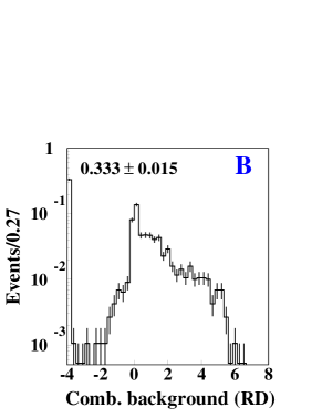
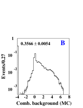
The variable ()
allows the two classes to be separated
(see Figure 1).
Variables, , are used
to separate the different classes of events with a real .
They are obtained from a measurement of the number of charged particle
tracks (excluding the charged lepton, the pion coming from the
and the decay products) which are
compatible with the -decay vertex or
with the main vertex.
For the signal (), it is expected that all other charged
particles in the
-jet are emitted from the
beam interaction region. This will be also true for (),
the remaining
background from events,
and for (). For the other
classes (, and ) it is expected that,
for most
of the events, one
or more additional charged particles are produced at the -vertex.
The variables are defined in the following way:
•
all charged particles, other than the decay products
and the lepton, emitted in the same event hemisphere
as the -candidate, with a momentum larger than 500 ,
which form a mass with the system lower than 6
and which have values for their impact parameters to the
-decay vertex smaller than 2 and 1.5 in and
respectively, are considered;
•
selected particles, having the same or the opposite
charge as the lepton are considered separately.
If there are several candidates in a class, the one with the
largest impact
parameter to the main vertex is retained and the quantity:
(11)
is evaluated,
where and are, respectively,
the sign and the number of standard deviations
for the track impact parameter relative to the main vertex.
The sign of the impact parameter is taken to be positive (negative)
if the corresponding track trajectory intercepts
the line of the jet axis from
the main vertex downstream (upstream) from that vertex.
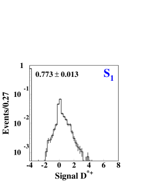
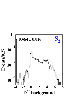
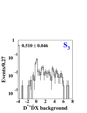
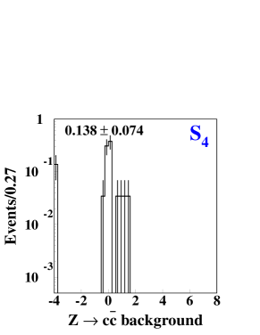
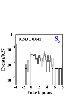
Figure 5: Distributions of the variable for signal and
background components. All distributions have been normalized to unity.
The content of the bin at has been inserted on each plot,
corresponding to events with no spectator track candidate.
In the two lower plots, distributions obtained for combinatorial
background events selected in real and simulated data can be compared.
For real data the distribution for
double charm cascade decays () has been corrected as described
in section 6.3.3.
As the track impact parameters can
extend to very large values because of the
relatively long decay time of -hadrons, the variables
are taken to be equal to the logarithm of and their
sign is taken to be the same as .
For events with no spectator track candidate, that is, with no additional
tracks compatible with the -decay vertex,
a fixed value of -4. is used for . Examples of
distributions of the variable for the signal and
for the different background components, corresponding
to all analysed channels,
are given in Figure 5.
Due to track reconstruction effects, only 77
of signal events have no spectator track candidate instead of the expected
100.
Similarly, for the background, 1/3 of
events with no additional
tracks are expected by isospin at the -vertex whereas 46 are observed.
These values allow the probabilities and
to be extracted for getting no spectator candidate
when, respectively, there is
not and when there is really such a candidate at generation level.
Values for these two probabilities
are respectively equal to
and with a spread of corresponding
to the different years and channels.
As it will be explained later (section 6.3.3),
these two quantities have been used to correct the present simulation
of
double charm cascade decays as it includes only the channel
whereas
the other contributions
() have a different charged particle topology.
6.3 Fitting procedures
Six event samples have been analysed separately
corresponding to different
detector configurations (1992-1993 and 1994-1995) and to
different decay channels of the
(, and ).
The analysis procedure is explained for a single such sample in the following
sections 6.3.1 to 6.3.7.
It is applied to all samples simultaneously to
obtain the measurements.
For each event , four measurements have been used:
.
The parameters
, and the
background from decays () are obtained by minimizing
a negative log-likelihood distribution.
Other parameters, given in the following, have to be introduced to account
for the various
fractions of contributing event classes and to describe their behaviour
in terms of the variables analysed.
The likelihood distribution is obtained from the product of the
probabilities to observe for each considered event.
These probabilities can be expressed in terms of the corresponding
probabilities for each event’s class and of their respective
contributions in the event samples analysed:
(12)
In this expression, and are the numbers of events
(fitted)
corresponding to the combinatorial background and to the different classes
of events with a real . The functions
and are the respective probability
distributions of
the variable .
Each probability distribution for the variable is considered to
be the product of four probability distributions corresponding
to the four different variables.
These distributions can be obtained from
data () or from the simulation.
The fitting procedure involves
minimizing the quantity:
(13)
where is the total number of events analysed.
From external measurements there are also constraints on the expected
number of events corresponding to the categories -.
These constraints can be applied assuming that the corresponding
event numbers follow Poisson distributions with fixed average values
().
This is obtained by adding to Equation (13) the quantity:
(14)
A similar expression is also added to account for the fact that
the total number of fitted events
must be compatible with the number () of selected events:
(15)
in which , the number of fitted events, is equal to:
.
The list of fitted parameters is given in the following for each
component contributing to the event sample analysed.
6.3.1 signal events
:
this distribution results from the convolution
of
the theoretical expected distribution
(corrected by the dependent efficiency and acceptance) with the
resolution function . It depends mainly on
and on the assumed dependence for the ratio
and between the different contributing form-factors.
:
is a Gaussian distribution
corresponding to the signal
for the
decay channels and a gamma distribution for
.
The two parameters for each distribution have been obtained from a fit to data.
:
these distributions are
obtained from simulated signal events. The two distributions,
for the and variables are rather similar with about
probability for having no spectator track candidate and
the remaining being concentrated around zero.
:
the number of signal events can be expressed as:
(16)
In this expression, is the number of hadronic events analysed
(Table 1),
is the fraction of hadronic decays into pairs,
the factor 4 corresponds to the two hemispheres and the fact that muons and
electrons
are used, is the production fraction of mesons in a -quark
jet,
is the semileptonic branching fraction of mesons which is measured in
this analysis,555 It is the integral of Equation 2
(divided by the total width) and depends
on the two fitted quantities and .
the other two branching fractions correspond, respectively,
to the selected
and decay channels (Table 10),
and are the
efficiencies, given in Table 4, of the cuts applied in
the analysis
to select signal events.
Note that is proportional to
.
6.3.2 events from decays
These are events from the class corresponding to the cascade decay
.
:
this distribution is taken from the simulation.
Its variation for different fractions of states has been studied
(see Section 7.3.4 and Figure 9)
and accounted for as a small systematic shift and error.
:
the same distribution
is used as for signal,
.
:
as for the signal,
these distributions are taken from the simulation.
It has been verified that they are not dependent on the type of
state which produced the . There is a marked
difference between and , the latter being
rather similar to the corresponding distribution for signal events.
:
the number of expected events
is fitted without imposing constraints from external measurements.
6.3.3 double charm cascade decay lepton events
These are events from the class corresponding to the cascade decay
:
this distribution is taken from the simulation.
:
the same distribution
is used as for signal,
.
:
when there are spectator tracks, the distribution
(with ), is used. The expected fractions of events with no spectator
tracks in the and distributions have been evaluated from the
measured contributions of
, and events
[12, 13],
with the branching fractions
and topological decay rates for the hadronic
states X, taken from [9].
For it is expected that of the events have no spectator
track and for this fraction is . These numbers have to
be corrected for reconstruction effects using the variables
and introduced in Section
6.2.
:
the expected number of events from this source is taken from
present measurements of decay rates
which correspond to:
(17)
where the lepton originates from the
semileptonic decay.
This value has been obtained using measurements from
ALEPH [12] and BaBar [13] on exclusive
double charm decay branching fractions of -hadrons,
with a charged emitted in the final state,
and using the inclusive semileptonic decay branching fractions of
charmed particles given in [9].
Simulated events contain double charm decays of the type
only,
with a corresponding
branching fraction:
.
This rate has been rescaled to correspond to the value
given in Equation (17), assuming that the experimental
acceptance is similar
for the different contributing channels.
6.3.4 events
:
this distribution is taken from the simulation.
:
the same distribution
is used as for signal,
.
:
as for the signal,
it is taken from the simulation.
:
the expected number of events from this source is taken from
the simulation after having corrected for the small difference between the
rates for production in -jets between simulated and real events
[14]:
(18)
The remaining contamination from is expected
to be very small (of the order of 1).
6.3.5 fake lepton events
Only fake lepton events associated with a real
and not coming from events, have to be considered
as the other contributions have been already included.
:
this distribution is taken from the simulation.
:
the same distribution
is used as for signal,
.
:
as for the signal,
it is taken from the simulation.
:
the expected number of events from this source is taken from
the simulation after
having applied corrections determined, using special event samples,
to account for
differences between the fake lepton rates in real and simulated data
(see Section 7.3).
6.3.6 semileptonic decays with a
These are events from the class corresponding to the cascade decay
:
this distribution is taken from the simulation.
:
the same distribution
is used as for signal,
.
:
is the same as the signal distribution
:
the expected number of events from this source is
obtained assuming that the production rate for -hadron semileptonic
decays is of the rate with a or [15]. As for the background, events
from decays are expected to give a small contribution,
of the order of .
6.3.7 combinatorial background events
Real data events are selected in the upper wing of the
mass peak between and
for channels,
and in the range for .
:
this distribution is taken from real data events located in the upper
part of the distribution.
:
the parametrization given in
Section 5.5 has been used.
The same mass dependence has been taken for the first four samples
while a parametrization corresponding to different values for the
coefficients has been obtained for events.
Parameters of these distributions have been fitted,
outside the global likelihood fit, to the
distributions corresponding to the events selected for the
analysis.
:
as for the distribution, the distributions for combinatorial
background events are obtained from analysed events, selecting those
situated in the upper part of the distribution.
:
in each of the six samples, the total number of
combinatorial
background events
is fitted over the total range.
7 Measurements of and
The six event samples have been analysed in the same way. Efficiencies
and
probability distributions have been
determined independently for each sample. Common parameters corresponding
to the description of physics processes have been fitted or taken from
external measurements. The central values and uncertainties
used for the latter are summarized in
Table 10.
7.1 Results on simulated events
Signal events generated using the DELPHI simulation program
correspond to a given dynamical model, using a given modelling of the
decay form factors. The generated distribution has been fitted
using a parametrization derived from the one
given in Section 2.
As the model used in the simulation is a priori different from
HQET
expectations, it has been necessary to add arbitrary terms
in the expression so that the fit will be reasonable over the whole
range.
These terms correspond to a polynomial development in powers of ,
starting with at least quadratic terms so that they have no effect
on the slope nor on the absolute value of the spectrum at the end-point
corresponding to .
Using the total number of generated events to fix the normalization,
the equivalent values
for the two parameters defining the signal in the simulation:
(19)
are obtained.
The fitted semileptonic branching fraction is equal to:
(20)
which agrees with the exact value of used to generate these events.
The exercise is repeated on pure signal events using the
reconstructed distribution. This predicted distribution
now includes the effects of the experimental reconstruction of the
variable and of the acceptance. This gives:
(21)
The fitted semileptonic branching fraction is equal to:
(22)
Finally, using the sample of
and simulated events,
the signal parameters are determined, including the different background
components giving (see Table 6):
(23)
The fitted semileptonic branching fraction is equal to:
(24)
demonstrating that the fitting procedure gives the expected values
for the signal parameters correctly.
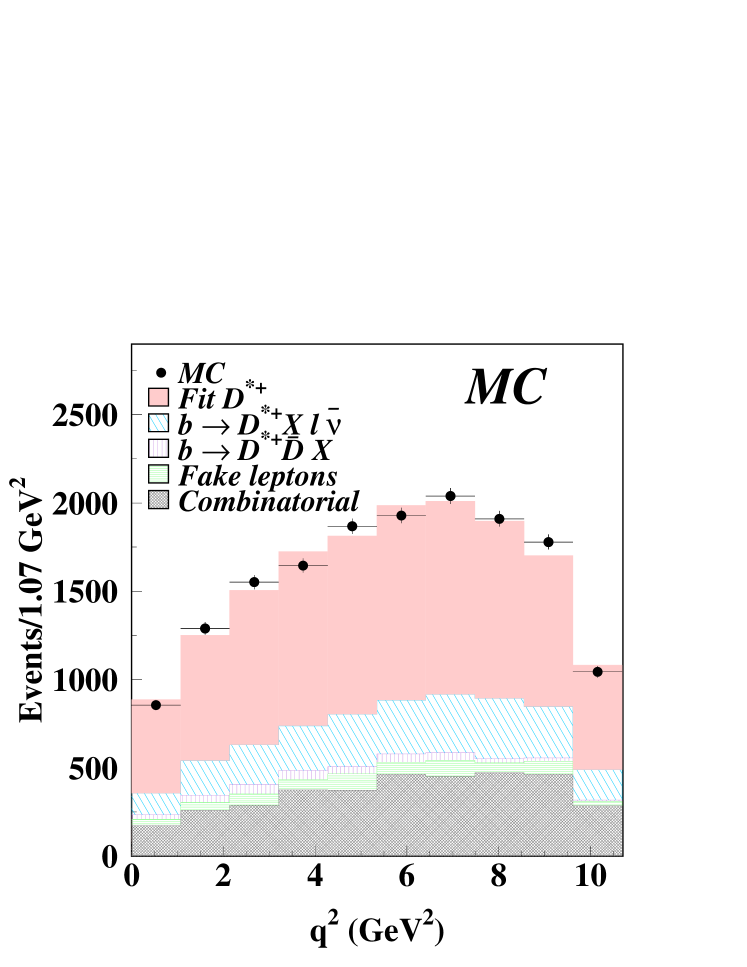
The distribution for MC events selected
within the interval for the and
channels and within the interval for is shown in Figure
6 with the
contributions from the fitted components.
Data set
92-93
0.0375 0.0020
1.27 0.17
5.16 0.21
94-95
0.0356 0.0013
1.16 0.13
4.94 0.14
92-93
0.0356 0.0020
1.03 0.21
5.28 0.23
94-95
0.0363 0.0014
1.13 0.13
5.20 0.15
92-93
0.0355 0.0018
1.14 0.17
4.95
0.19
94-95
0.0351 0.0013
1.05 0.13
5.06
0.14
Total sample
0.03579 0.00063
1.122 0.061
5.081 0.065
Table 6: Fitted values of the parameters in simulated events.
The quoted uncertainties are statistical.
Figure 6: Fit of MC and events.
The three analysed decay channels and the two data taking periods
have been combined. Only events selected within the
mass interval corresponding to the signal are displayed.
The small contribution of
decays and leptons originating from events has been
included in the fake lepton component.
7.2 Results from data
To analyse real data events, additional corrections have been applied
to account for remaining differences between real and simulated events.
Central values and uncertainties on these corrections are explained
in the following when evaluating systematic uncertainties attached
to the present measurements.
The results obtained on the six data samples and using the total
statistics are
given in Table 7.
Data set
92-93
0.0394 0.0055
1.15 0.48
6.55 0.77
94-95
0.0340 0.0041
0.71 0.45
6.11 0.55
92-93
0.0410 0.0058
1.43 0.46
6.06 0.77
94-95
0.0342 0.0042
1.12 0.41
5.01 0.51
92-93
0.0407 0.0043
1.36 0.35
6.22 0.57
94-95
0.0404 0.0031
1.48 0.24
5.70 0.40
Total sample
Table 7: Fitted values of the parameters on real data events.
The quoted uncertainties are statistical.
As 92-93 event samples have a reduced sensitivity to the
background (S2), fitted values quoted in this Table, when corresponding to
individual event samples, have been obtained using a fixed value for the
branching fraction
(=0.67 , see Equation 29). Results quoted for the
total statistics have been obtained letting free this quantity
to vary in the fit.
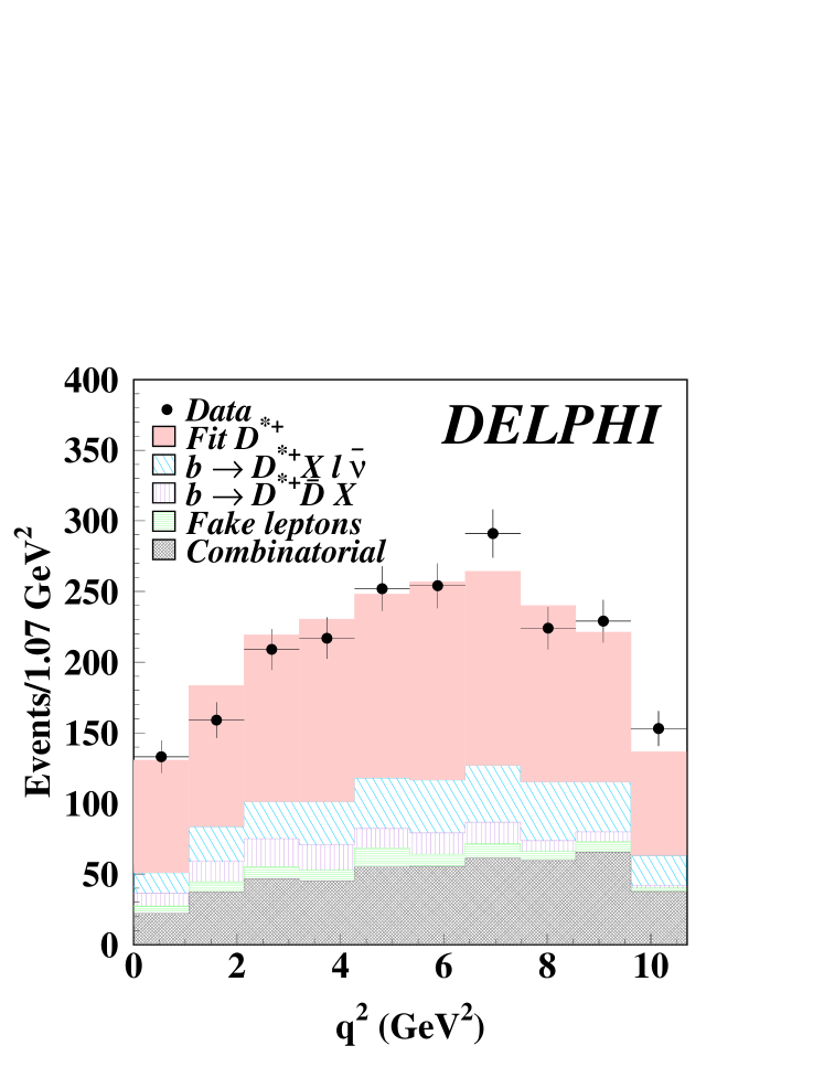
Figure 7: Fit on real data events. All periods are combined.
Only events selected within the
mass interval corresponding to the signal are displayed.
The small contribution of
decays and leptons originating from events has been
included in the fake lepton component.
The values obtained are:
(25)
which correspond to a branching fraction equal to:
(26)
The correlation coefficient
is equal to 0.894.
Fitted fractions of the different components
are given in Table 8.
Distributions of the and variables for events selected
within the interval for the and
channels and within the interval for are shown in Figures
7 and 8 with the
contributions from the fitted components.
Signal
Cascade
Charm
Fake lept.
Comb. Backg.
()
()
()
()
()
()
B
Table 8: Number of events
and fitted fractions
(in of signal events) attributed to the different
components of the analysed sample of
events selected within the mass interval
corresponding to the signal.
Figure 8: Distributions for the variables, for events selected
within the
interval of the signal and corresponding
contributions from the fitted
components. The small contribution of
decays and leptons originating from events has been
included in the fake lepton component.
The measured (fitted) number of events in the first bin, at
-4., are
1324 36 (1358) and 1498 39 (1540), for the and
distributions respectively.
7.3 Evaluation of systematic uncertainties
Values for the parameters taken from external measurements and hypotheses
used in the present analysis have been varied within their corresponding
range of
uncertainty. The results are summarized in Table 9.
Table 9: Systematic uncertainties given as relative values
expressed in . The total systematics are obtained by summing the
components in quadrature.
7.3.1 Uncertainties related to external parameters
parameter
central value
or hypothesis
and uncert.
Rb
P()
BR
BR
BR
BR
BR
BR
Table 10: Values for the external parameters used in the analysis.
The quoted value for BR corresponds
to the sum of the branching fractions for the electron and muon final states.
•
Values for D and branching fractions into the analysed
final states, the Rb value and the -hadron lifetime have been
taken from [9].
A summary of the values used in the present analysis is given in
Table 10. They have been varied within
the corresponding range of uncertainty and the systematic errors
induced in ,
and the are given in Table 11.
•
Global efficiencies to select events
have been estimated using the simulation as described in section
5.4. Measured branching fractions of several decay channels have been used for real data and a correction factor has
been applied to take into account events from undetermined origin.
•
Simulated events have been generated using the JETSET 7.3 program
with the parton shower option [11]. The non-perturbative
part of the fragmentation of -quark jets is taken to be a Peterson
distribution which depends
on a single parameter, :
(27)
In this expression, is a normalization factor and
with and indicating the
B hadron and the -quark. The average fraction of the beam energy taken
by weakly decaying -hadrons has been evaluated in [14] to be
. Simulated events,
generated with the parameter ,
correspond to .
The effects of a variation of the average
value and of the shape of the fragmentation distribution,
on the results of the analysis have been studied by weighting
events generated with a known value of the variable
so that they correspond to recent measurements [16].
In addition to a change in the slope of the B momentum distribution,
increases by 2.
A new parametrization of the resolution function
described in section 5.6
has been determined on simulated weighted events and the analysis has
been redone giving relative variations of and ,
respectively, on and .
•
The -hadron lifetime used in the simulation is equal to
and is independent of the type of produced -hadrons. Events have been
weighted so that their lifetime agrees with present measurements.
Efficiencies given in Table 4 have been
determined using weighted
events and uncertainties related to the present accuracy on the
lifetime measurement can be neglected.
parameter
rel. err. on
rel. err. on
rel. err. on
or hypothesis
BR
Rb
0.15
0.01
0.32
P()
1.69
0.02
3.39
BR
0.37
0.03
0.76
BR
0.31
0.01
0.63
BR
0.68
0.0
1.35
BR
1.70
0.35
3.64
Total
2.5
0.4
5.3
Table 11: Systematic uncertainties from external parameters as
relative values expressed in . The uncertainty
related to the BR
includes the contribution of the ,
and
branching fractions.
Central values and errors of these parameters are given
in Table 10.
7.3.2 Uncertainties from the detector performance
•
Differences between simulated and real data events on the tracking
efficiency have been studied in [17] and correspond
to for each charged particle. For the soft pion
coming from the an uncertainty of has been assumed.
•
Differences between simulated and real data events on lepton
identification have been measured using dedicated samples of real data events
[18] and the real data to simulation ratios are equal to
( and (
for electrons. For muons, the real data to simulation ratios are equal to
for the two periods with a uncertainty.
•
Differences between fake lepton rates in which the
lepton is a misidentified hadron, have also been measured
using dedicated samples of real data events and compared with the simulation
[18]
to obtain correction factors which are summarized in Table 12.
Data set
electron
muon
92-93
94-95
Table 12: Correction factors to apply to simulated events
in which the candidate lepton is a misidentified hadron.
•
Resolution of the variable.
A resolution function, common to all three decay channels has been used.
This function is determined independently for the 92-93 and 94-95 data
samples. To quantify the importance of controlling the experimental resolution
on the widths of the fitted Gaussians have been increased by
5.
This value is two times larger than observed differences between the averaged
missing energy measured in jets for real and simulated events. It
corresponds to the increase in smearing of the resolution
function when including events with a missing .
The induced variations in
and
are and respectively.
The uncertainty on the parametrization of the resolution
distributions has been evaluated by varying the number of fitted
groups of slices in on which a linear variation of the parameters
of the two Gaussian distributions were evaluated. Results
obtained with two groups of 10 slices and with five groups
of four slices have been compared. This corresponds to relative variations on
and
of and respectively.
Results obtained when
including or excluding events,
which have a poorer resolution, in the determination
of the resolution function have been also compared.
This corresponds to relative variations on
and
of and respectively.
Measured differences obtained from these comparisons have
been summed in quadrature.
The value of is obtained from the measurements of the B and
4-momenta (see Section 5.6). The B momentum is obtained from a
constrained fit, imposing the B meson mass, which includes information
from primary and secondary vertex positions and from the energy
and momentum of
the particles belonging to the jet that provide an estimate of the B momentum
and direction. Uncertainties on the polar and azimuthal angles giving the
B direction, and on the magnitude of the B momentum, which were determined
from the measurement of the , charged lepton and missing-jet momenta,
have been varied by and new resolution distributions
for have been
obtained.
Corresponding variations on fitted values for
and are found to be negligible.
•
Control of the distributions.
Distributions of the variables obtained for events selected
for values of higher than the signal, in real
and simulated events, have been compared (see the bottom two
distributions in Figure 5). The probabilities
for having no spectator track differ by between data
and the simulation. To account for this difference the corresponding
probabilities for no spectator track have been varied by ,
simultaneously for signal and background components with a
real . Such a variation does not apply for events
from the combinatorial background as the shape of the corresponding
distributions has been taken from real events.
The effect of a different shape of the distributions
has also been evaluated for double charm cascade decays .
A flat distribution has been considered for to account
for the different topologies of , and
. The effect of this variation has been found
to be negligible.
•
The effect of a possible difference between the tuning of
the -tagging
[10]
between real and simulated data events has been neglected
because loose criteria have been used in this analysis.
7.3.3 Uncertainties on signal modelling
These uncertainties correspond to the use of the dependent
ratios and defined in Equation (7).
Values for these quantities, using different models, have been obtained
by the CLEO collaboration [4]: ,
with a correlation between
the uncertainties on these two measurements. Relative variations induced in
the fitted parameters
, and have been obtained varying
the values of and within their corresponding range of uncertainty.
They are given in Table 13.
1.3
0.3
0.0
1.8
22.5
0.0
Table 13: Relative variations of the fitted parameters due to the
and measurements. The 1 variation corresponds to the sum
in quadrature of the statistical and systematic uncertainties.
As observed already in previous analyses, the uncertainty on
dominates the systematic uncertainty on .
7.3.4 Uncertainties on background modelling
•
The fraction of mesons originating from decays of
mesons depends on the total production rate of these states and on their
relative fractions.
Combining present measurements, the production rate of mesons
originating from decays and
accompanied by an opposite sign lepton is [14]:
(28)
This information is not included in the fit as events produced
in decays are directly fitted,
simultaneously with and ,
to the data giving:
(29)
which is compatible with the expectation given in
Equation (28).
The statistical error correlation coefficients
are:
and .
The quoted systematic, in Equation (29), has been evaluated
by considering the same sources of errors as are listed in
Table 9.
To evaluate the effect of the uncertainty in the sample composition
of produced states, the model of [19] has been used.
Parameters entering into this model have been varied so that the
corresponding production rates of the narrow states remain within the
measured ranges
defined in Equations (30, 31):
(30)
(31)
(32)
where is the ratio between the production rates
of and
in -meson semileptonic decays.
A dedicated simulation program has been written to generate the
decay distributions of the different states. Correlations between
the lepton and hadron momenta induced by the decay dynamics are included.
The dependence of the different form factors has been parametrized
according to the model given in [19]. It has been assumed
that, in addition to narrow states whose production fractions
are given in Equations (30-32), broad
final states, emitted in a relative S wave, are produced.
The two sets of model parameters giving the two most displaced central
values for the distribution are used to evaluate the systematic
uncertainty coming from the sample composition of
states666 Values of the parameters (see [19])
corresponding to Model 1 are:
. The corresponding values for Model 2 are:
..
These two distributions
are shown in Figure 9 and the fitted values
obtained with these two models are given in Table 14.
Model 1
Model 2
Table 14: Fitted values corresponding to the two models describing
production.
The average of these two results is used
to determine the central values for and
and half of their difference is taken as systematic
uncertainty; this gives:
.
Figure 9: distributions, normalized to unity,
obtained using the two sets of
parameters of the model [19], which correspond
to the largest variation in the central value of these distributions
and which give production rates for narrow states that are
compatible with present measurements. The precise definition
for models 1 and 2 is given in section 7.3.4.
The three components given in each
histogram correspond, from top to bottom, to narrow 2+, broad
1+ and narrow 1+ states.
•
The rate for the double charm cascade decay background, evaluated from
simulated events,
has been rescaled to agree with present measurements
(see Equation (17)).
•
The small components of tau and charm backgrounds have been evaluated using
present measurements.
•
The modelling uncertainty of the combinatorial component corresponding
to events situated under the peak has a negligible contribution.
8 Combined result
The present measurement of and has been
combined with the previous DELPHI result [20]
obtained with a more inclusive analysis in which the was
reconstructed using the charged pion and tracks attached
to a secondary vertex, accounting for the decay products. The values
obtained in the previous DELPHI analysis were:
and
.
Modifying the central values and uncertainties of the parameters entering in
this analysis so that they correspond to the
values taken for the present measurement yields the results:
and
.
The average with the present measurement
has been obtained using the method adopted by the LEP Vcb
working group [14].
Common sources of systematic uncertainties between the two analyses have
also been identified and properly treated in the averaging procedure.
The statistical correlation between the two measurements has been
evaluated to be 8 (it was evaluated to be 5 in
[2] where a similar combination was done).
Averaging the two measurements gives the following results:
and
.
Using gives:
,
where the last uncertainty corresponds to the systematic error from
theory.
9 Conclusions
Measurements of ,
and of
have been obtained using exclusively reconstructed
decays by the DELPHI Collaboration. Variables have been defined
which allow different decay mechanisms producing mesons in the
final state to be separated.
The following values have been obtained:
,
which correspond to a branching fraction:
.
These values are in agreement with previous measurements obtained
by the ALEPH [21], DELPHI [20] and
OPAL [22] collaborations.
The -quark semileptonic branching fraction into a emitted
from higher mass charmed excited states has also been measured to be:
.
Combining the present measurements with the previous analysis from DELPHI
[20] which was done
using a more inclusive approach, yields:
and
.
Using this gives:
,
where the last uncertainty corresponds to the systematic error from
theory.
Acknowledgements
We are greatly indebted to our technical
collaborators, to the members of the CERN-SL Division for the excellent
performance of the LEP collider, and to the funding agencies for their
support in building and operating the DELPHI detector. We acknowledge in particular the support of Austrian Federal Ministry of Education, Science and Culture,
GZ 616.364/2-III/2a/98, FNRS–FWO, Flanders Institute to encourage scientific and technological
research in the industry (IWT), Federal Office for Scientific, Technical
and Cultural affairs (OSTC), Belgium, FINEP, CNPq, CAPES, FUJB and FAPERJ, Brazil, Czech Ministry of Industry and Trade, GA CR 202/99/1362, Commission of the European Communities (DG XII), Direction des Sciences de la Matire, CEA, France, Bundesministerium fr Bildung, Wissenschaft, Forschung
und Technologie, Germany, General Secretariat for Research and Technology, Greece, National Science Foundation (NWO) and Foundation for Research on Matter (FOM),
The Netherlands, Norwegian Research Council, State Committee for Scientific Research, Poland, SPUB-M/CERN/PO3/DZ296/2000,
SPUB-M/CERN/PO3/DZ297/2000 and 2P03B 104 19 and 2P03B 69 23(2002-2004) JNICT–Junta Nacional de Investigação Científica
e Tecnolgica, Portugal, Vedecka grantova agentura MS SR, Slovakia, Nr. 95/5195/134, Ministry of Science and Technology of the Republic of Slovenia, CICYT, Spain, AEN99-0950 and AEN99-0761, The Swedish Natural Science Research Council, Particle Physics and Astronomy Research Council, UK, Department of Energy, USA, DE-FG02-01ER41155, EEC RTN contract HPRN-CT-00292-2002.
References
[1]
A.F. Falk and M. Neubert, Phys. Rev. D47 (1993) 2965 and 2982;
T. Mannel, Phys. Rev. D50 (1994) 428;
M.A. Shifman, N.G. Uraltsev and A.I. Vainshtein, Phys. Rev. D51 (1995)
2217, Erratum-ibid. D52 (1995) 3149.
[2]
P. Abreu et al., DELPHI Collaboration, Z. Phys. C71 (1996) 539.
[3]
M. Neubert, Phys. Rept. 245 (1994) 259-396.
[4]
J.E. Dubosq et al., CLEO Collaboration, Phys. Rev. Lett. 76 (1996)
3898.
[5] I. Caprini, L. Lellouch and M. Neubert, Nucl. Phys. B530
(1998) 153.
[6]
C.G. Boyd, B. Grinstein and R.F. Lebed, Phys. Rev. D56 (1997) 6895.
[7]
N. Isgur and M. Wise, Phys. Lett. B232 (1989) 113;
N. Isgur and M. Wise, Phys. Lett. B237 (1990) 527.
[8]
A. F. Falk, H. Georgi, B. Grinstein and M. B. Wise, Nucl.
Phys. B343 (1990) 1.
[9]
Particle Data Group, K. Hagiwara et al., Phys. Rev. D66 (2002)
010001.
[10]
DELPHI Collaboration, P. Abreu et al., Nucl. Instr. Meth. A378
(1996) 57.
[11]
T. Sjöstrand, Comp. Phys. Comm. 82 (1994) 74.
[12]
R. Barate et al., ALEPH Collaboration, Eur. Phys. J. C4 (1998) 387.
[13]
B. Aubert et al., BaBar Collaboration, SLAC-PUB-9736, hep-ex/0305003.
[14]
Combined results on -hadron production rates, lifetimes, oscillations
and semileptonic decays (ALEPH, CDF, DELPHI, L3, OPAL, SLD),
CERN-EP/2001-050, hep-ex/0112028.
[15]
A.H. Hoang, Z. Ligeti and A.V. Manohar, Phys. Rev. D59 (1999) 074017.
[16]
ALEPH Collaboration, Phys. Lett. B512 (2001) 30.
[17]
P. Abreu et al., DELPHI Collaboration, Phys. Lett. B425 (1998)
399.
[18]
P. Abreu et al., DELPHI Collaboration. Eur. Phys. J C20 (2001)
455.
[19]
A.K. Leibovich, Z. Ligeti, I.W. Stewart and M.B. Wise, Phys. Rev D57
(1998) 308.
[20] P. Abreu et al., DELPHI Collaboration,
Phys. Lett. B510 (2001) 55.
[21] D. Buskulic et al., ALEPH Collaboration, Phys.
Lett.
B395 (1997) 373.
[22]
G. Abbiendi et al., OPAL Collaboration, Phys. Lett. B482 (2000)
15.