Constraints on Neutrino Mixing Parameters with the SNO data

Abstract

This paper reviews the constraints imposed on the solar neutrino mixing parameters by data collected by the Sudbury Neutrino Observatory (SNO). The SNO multivariate analysis is reviewed. The global solar neutrino analysis is emphasized in terms of matter-enhanced oscillation of two active flavors. An outline of how SNO uses the data to produce oscillation contour plots and how to include the relevant correlations for the new salt data in similar oscillation analyses is summarized.

I Introduction

The deficit of detected neutrinos coming from the Sun compared with our expectations based on laboratory measurements, known as the Solar Neutrino Problem, was one of the outstanding problems in basic physics for over thirty years. It appeared inescapable that either our understanding of the energy producing processes in the Sun was seriously defective, or neutrinos, one of the fundamental particles in the Standard Model, had important properties which had not been measured. It was indeed argued by some that we needed to change our ideas on how energy was produced in fusion reactions inside the Sun. Others suggested that the problem arose due to peculiar characteristics of neutrinos such as vacuum or matter oscillations. It is useful to review the evolution of our understanding from the data collected by various solar neutrino experiments. The new analysis of the salt data collected by the Sudbury Neutrino Observatory (SNO) bib:snosalt will be described, together with the technique used to combine the results of many solar neutrino experiments.

II Solar Neutrinos

The energy in the Sun is produced by nuclear reactions that transform hydrogen into helium. Through the fusion reactions, four protons combine to form a helium nucleus containing two protons and two neutrons. The only reactions that allow this to happen are caused by weak interactions like nuclear beta decay. Each time a neutron is formed, there must be an associated positron and electron neutrino produced. Neutrinos can travel directly from the core of the Sun to the Earth in a about eight minutes and hence provide a direct way to study thermonuclear processes in the Sun. The detailed predictions of the solar electron neutrino flux have been produced by John Bahcall and his collaborators from the 1960’s until now. Their calculations are refereed to as the Standard Solar Model (SSM). In this proceeding, the Bahcall-Pinsonneault calculations bib:BP are compared to experimental results.

It is known that neutrinos exist in different flavors corresponding to the three charged leptons: the electron, muon, and tau particles. If neutrinos have masses, flavor can mix and a neutrino emitted in a weak interaction is represented as a superposition of mass eigenstates. In the case of three flavors of neutrino, the mixing matrix $U$ is called the Maki-Nakagawa-Sakata-Pontecorvo (MNSP) matrix bib:mnsp and $\nu_{\ell}=\sum_{i}U_{\ell i}|\nu_{i}\rangle$. Here the neutrino mass eigenstates are denoted by $\nu_{i}$ with $i=1,2,3$, while the flavor eigenstates are labeled $(e,\mu,\tau)$. The most general form of mixing for three families of neutrinos can be simplified so that only two neutrinos participate in the oscillations. Hence, the survival probability for solar neutrinos propagating in time takes the approximate form

$$P_{e\beta}=\delta_{e\beta}-(2\delta_{e\beta}-1)\sin^{2}2\theta\sin^{2}(1.27\frac{\Delta m^{2}L}{E})\,.$$ (1)

The mixing angle is represented by $\theta$, $L$ is the distance between the production point of $\nu_{e}$ and the point of detection of $\nu_{\beta}$, E is the energy of the neutrino, and $\Delta m^{2}\equiv m^{2}_{j}-m^{2}_{i}$ is the difference in the squares of the masses of the two states $\nu_{j}$ and $\nu_{i}$ which are mixing. The function $\delta_{e\beta}$ is the usual Kronecker delta. The numerical constant 1.27 is valid for $L$ in meters, $E$ in MeV, and $\Delta m^{2}$ in eV². The energy of a neutrino depends on the type of nuclear reaction which produced it. By studying the evolution of the solar neutrinos as a function of $L$, all the physics is embedded in one angle $\theta$, one mass difference $\Delta m^{2}$, and the sign of $\Delta m^{2}$. This corresponds to the extraction of the three MNSP elements: $U_{e1}$, $U_{e2}$, and $U_{e3}$.

III Sudbury Neutrino Observatory

The Sudbury Neutrino Observatory (SNO) is a 1,000 ton heavy-water $\check{\rm{C}}$erenkov detectorbib:snonim situated 2 km underground in INCO’s Creighton mine in Canada. Another 7,000 tons of ultra-pure light water is used for support and shielding. The heavy water is in an acrylic vessel (12 m diameter and 5 cm thick) viewed by 9,456 PMT mounted on a geodesic structure 18 m in diameter; all contained within a polyurethane-coated barrel-shaped cavity (22 m diameter by 34 m high). The solar-neutrino detectors in operation prior to SNO were mainly sensitive to the electron neutrino type; while the use of heavy water by SNO allows neutrinos to interact through charged-current (CC), elastic-scattering (ES), or neutral-current (NC) interactions. The determination of these reaction rates is a critical measurement in determining if neutrinos oscillate in transit between the core of the Sun and their observation on Earth.

During the pure $D_{2}O$ phase of the experiment, the signal was determined with a statistical analysis based on the direction, $\cos\theta_{\rm{sun}}$, the position, $R$, and the kinetic energy, $T$, of the reconstructed events assuming the SSM energy spectrum shape bib:ortiz . The final selection criteria were $T\geq 5$ MeV and $R\leq 550$ cm. The result of the extended maximum-likelihood fit yields bib:snod2o

$$\Phi_{\rm{CC}} = 1.76\,^{+0.06}_{-0.05}\,{}^{+0.09}_{-0.09}\,\times 10^{6}~{}{\rm cm}^{-2}{\rm s}^{-1}\,,$$

$$\Phi_{\rm{ES}} = 2.39\,^{+0.24}_{-0.23}\,{}^{+0.12}_{-0.12}\,\times 10^{6}~{}{\rm cm}^{-2}{\rm s}^{-1}\,,$$ (2)

$$\Phi_{\rm{NC}} = 5.09\,^{+0.44}_{-0.43}\,{}^{+0.46}_{-0.43}\,\times 10^{6}~{}{\rm cm}^{-2}{\rm s}^{-1}\,.$$

The excess of the NC flux over the CC and ES fluxes implies neutrino flavor transformations. There is also a good agreement between the SNO NC flux and the total ${}^{8}B$ flux of $5.05^{+1.01}_{-0.81}$ $\times 10^{6}~{}{\rm cm}^{-2}{\rm s}^{-1}$ predicted by the SSM. A simple change of variables that resolves the data directly into electron and non-electron components bib:snod2o indicates clear evidence of solar neutrino flavor transformation at 5.3 standard deviations

$$\phi_{e} = 1.76\,^{+0.06}_{-0.05}\,{}^{+0.09}_{-0.09}\,\times 10^{6}~{}{\rm cm}^{-2}{\rm s}^{-1}\,,$$ (3)

$$\phi_{\mu\tau} = 3.41\,^{+0.45}_{-0.45}\,{}^{+0.48}_{-0.45}\,\times 10^{6}~{}{\rm cm}^{-2}{\rm s}^{-1}\,.$$ (4)

Allowing a time variation of the total flux of solar neutrinos leads to day/night measurements by SNO, which are sensitive to the neutrino type bib:snoDN

$$A_{\rm{DN}}({\rm{total}})=(-24.2\pm 16.1\,^{+2.4}_{-2.5})\,\%\,,$$ (5)

$$A_{\rm{DN}}(e)=(12.8\pm 6.2\,^{+1.5}_{-1.4})\,\%\,.$$ (6)

By forcing no asymmetry in the $\phi_{e}+\phi_{\mu\tau}$ rate, i.e. $A_{\rm{DN}}({\rm{total}})=0$, the day/night asymmetry for the electron neutrino is bib:snoDN $A_{\rm{DN}}(e)=(7.0\pm 4.9\,^{+1.3}_{-1.2})$.

SNO published its first results of the salt phase bib:snosalt in coincidence with the PHYSTAT2003 conference. The measurements were made with dissolved $NaCl$ in the heavy water to enhance the sensitivity and signature for neutral-current interactions. Neutron capture on ${}^{35}Cl$ typically produces multiple $\gamma$ rays while the CC and ES reactions produce single electrons. The greater isotropy of the $\check{\rm{C}}$erenkov light from neutron capture events relative to CC and ES events allows good statistical separation of the event types. The degree of the $\check{\rm{C}}$erenkov light isotropy is determined by the pattern of PMT hits. This separation allows a precise measurement of the NC flux to be made independent of assumptions about the CC and ES energy spectra. To minimize the possibility of introducing biases, SNO performed a blind analysis for the model independent determination of the total active ${}^{8}B$ solar neutrino. In this analysis, events are statistically separated into CC, NC, ES, and external-source neutrons using an extended maximum-likelihood technique based on the distributions of isotropy, $\cos\theta_{\rm{sun}}$, and radius, R, within the detector. To take into account correlations between isotropy and energy, a 2D joint probability density function (PDF) is constructed. This analysis differs from the analyses of the pure $D_{2}O$ data bib:snod2o ; bib:snoDN since (1) correlations are explicitly incorporated in the signal extraction and (2) the spectral distributions of the ES and CC events are not constrained to the ${}^{8}B$ shape, but are extracted from the data. $\check{\rm{C}}$erenkov event backgrounds from $\beta-\gamma$ decays are reduced with an effective electron kinetic energy threshold $T$ $\geq$ 5.5 MeV and a fiducial volume with radius $R\leq 550$ cm.

The extended maximum-likelihood analysis gives the following ${}^{8}B$ fluxes bib:snosalt

$$\Phi_{\rm{CC}} = 1.59\,^{+0.08}_{-0.07}\,{}^{+0.06}_{-0.08}\,\times 10^{6}~{}{\rm cm}^{-2}{\rm s}^{-1}\,,$$

$$\Phi_{\rm{ES}} = 2.21\,^{+0.31}_{-0.26}\pm{0.10}\,\times 10^{6}~{}{\rm cm}^{-2}{\rm s}^{-1}\,,$$ (7)

$$\Phi_{\rm{NC}} = 5.21\pm 0.27\pm 0.38\,\times 10^{6}~{}{\rm cm}^{-2}{\rm s}^{-1}\,.$$

The systematic uncertainties on the derived fluxes are shown in Table 1. These fluxes are in agreement with previous SNO measurements and the SSM. The ratio of the ${}^{8}B$ flux measured with the CC and NC reactions then provides confirmation of solar neutrino oscillations

$$\frac{\Phi_{\rm{CC}}}{\Phi_{\rm{NC}}}=0.306\pm 0.026\pm 0.024\,.\\$$ (8)

Source	NC	CC	ES
Energy scale	-3.7,+3.6	-1.0,+1.1	$\pm 1.8$
Energy resolution	$\pm 1.2$	$\pm 0.1$	$\pm 0.3$
Energy non-linearity	$\pm 0.0$	-0.0,+0.1	$\pm 0.0$
Radial accuracy	-3.0,+3.5	-2.6,+2.5	-2.6,+2.9
Vertex resolution	$\pm 0.2$	$\pm 0.0$	$\pm 0.2$
Angular resolution	$\pm 0.2$	$\pm 0.2$	$\pm 2.4$
Isotropy mean	-3.4,+3.1	-3.4,+2.6	-0.9,+1.1
Isotropy resolution	$\pm 0.6$	$\pm 0.4$	$\pm 0.2$
Radial energy bias	-2.4,+1.9	$\pm 0.7$	-1.3,+1.2
Vertex Z accuracy	-0.2,+0.3	$\pm 0.1$	$\pm 0.1$
Internal neutrons	-1.9,+1.8	$\pm 0.0$	$\pm 0.0$
Internal background	$\pm 0.1$	$\pm 0.1$	$\pm 0.0$
Neutron capture	-2.5,+2.7	$\pm 0.0$	$\pm 0.0$
$\check{\rm{C}}$erenkov backgrounds	-1.1,+0.0	-1.1,+0.0	$\pm 0.0$
AV events	-0.4,+0.0	-0.4,+0.0	$\pm 0.0$
Total uncertainty	-7.3,+7.2	-4.6,+3.8	-4.3,+4.5

Table 1: Systematic uncertainties (in %) on fluxes for the spectral shape unconstrained analysis of the salt data set.

IV How to Use the SNO Data

The SNO CC, ES and NC fluxes are statistically correlated, since they are derived from a fit to a single data set. The statistical correlation coefficients between the fluxes in the salt phase are

$$\rho_{{\rm{CC,NC}}} = -0.521\,,$$

$$\rho_{{\rm{CC,ES}}} = -0.156\,,$$ (9)

$$\rho_{{\rm{ES,NC}}} = -0.064\,.$$

These can be used with the statistical uncertainties quoted by SNO bib:snosalt to write down the statistical covariance matrix for the salt fluxes. Systematic uncertainties between fluxes can be correlated as well. Some sources of systematic error, such as neutron capture efficiency, affect only one of the three fluxes, and so can be considered to be uncorrelated with the other fluxes. Other systematics can be either 100% correlated (e.g. radial accuracy) or 100% anticorrelated (e.g. isotropy mean). The most important anti-correlated systematic is the isotropy mean. Isotropy is important for separating CC and ES events from NC events, so CC and ES will have a negative correlation with the NC flux (and a positive correlation with each other) for the isotropy uncertainty. Table 2 shows the sign of the correlation for each systematic of Table 1. Using the table of systematics and the signs for the correlations, one can assemble an individual covariance matrix for each systematic. Then, to get the total covariance matrix for the CC, ES and NC fluxes, one simply adds all of the covariance matrices together.

Even when fluxes are being analyzed as opposed to energy spectra, it is best to determine the effect of energy-related systematics at each grid point in the $\Delta m^{2}-\tan^{2}\theta$ plane. For the salt analysis, these include energy scale and energy resolution; the uncertainty due to energy non-linearity is tiny so that it can reasonably be ignored. The energy scale uncertainty is implemented as a 1.1% uncertainty in the total energy; while the energy resolution has an uncertainty which is energy dependent for $T>4.975$ MeV

$$\frac{\Delta\sigma_{T}}{\sigma_{T}}=0.035+0.00471\times(T-4.975)\,,$$ (10)

and $\frac{\Delta\sigma_{T}}{\sigma_{T}}=0.034$ for $T<4.975$ MeV. Here $T$ is the reconstructed kinetic energy. For all other systematics, it is assumed that the effect on the fluxes is the same for all oscillation parameters.

Source	NC	CC	ES
Energy scale	+1	+1	+1
Energy resolution	+1	+1	+1
Energy non-linearity	+1	+1	+1
Radial accuracy	+1	+1	+1
Vertex resolution	+1	+1	+1
Angular resolution	+1	+1	– 1
Isotropy mean	+1	– 1	– 1
Isotropy resolution	+1	+1	+1
Radial energy bias	+1	+1	+1
Vertex X accuracy	+1	+1	+1
Vertex Y accuracy	+1	+1	+1
Vertex Z accuracy	+1	– 1	– 1
Internal neutrons	+1	0	0
Internal background	+1	+1	+1
Neutron capture	+1	0	0
$\check{\rm{C}}$erenkov backgrounds	+1	+1	+1
AV events	+1	+1	+1

Table 2: Signs of systematic correlations, relative to its effect on the NC flux. An entry of $+1$ indicates a 100% positive correlation, $-1$ a 100% negative correlation, and $0$ means no correlation.

When SNO quotes $\Phi_{\rm{CC}}=1.59\times 10^{6}~{}{\rm cm}^{-2}{\rm s}^{-1}$, it refers to the integral flux from zero to the endpoint assuming an undistorted ${}^{8}B$ spectrum. It implies that the number of events attributed to CC interactions above $T=5.5$ MeV is equal to the number of events that would be observed if the $\nu_{e}$ flux follows the ${}^{8}B$ spectral shape. The ${}^{8}B$ spectral shape aspect of this definition is only for normalization; there is no assumption of any spectral shape when extracting the number of events during the salt phase. Similar definitions apply for the NC and ES fluxes.

For the comparison of the SNO CC rate with the theoretical rates for a set of oscillation parameters, the $\Phi_{\rm{CC}}$ flux is

$$f_{B}\int_{0}^{\infty}\phi_{\rm{SSM}}(E_{\nu})\,dE_{\nu}\,S(T,T_{e},E_{\nu})\,,$$ (11)

with the scale $S(T,T_{e},E_{\nu})$ is equal to

$$\frac{\int_{0}^{\infty}\int_{0}^{\infty}\int_{5.5}^{\infty}F(T,T_{e},E_{\nu})P_{ee}(E_{\nu})dTdT_{e}dE_{\nu}}{\int_{0}^{\infty}\int_{0}^{\infty}\int_{5.5}^{\infty}F(T,T_{e},E_{\nu})dTdT_{e}dE_{\nu}}\,,$$ (12)

where

$$F(T,T_{e},E_{\nu})=\phi_{\rm{SSM}}(E_{\nu})\,\frac{d\sigma(E_{\nu},T_{e})}{dT_{e}}\,N(T_{e},\sigma^{2}_{T})\,.$$ (13)

The factor $f_{B}$ allows the total ${}^{8}B$ solar neutrino flux to float from the SSM value, $E_{\nu}$ is the neutrino energy, $P_{ee}$ is the survival probability, $T_{e}$ is the true recoil electron kinetic energy, and $T$ is the observed electron kinetic energy; while $N(T_{e},\sigma^{2}_{T})$ is a Gaussian energy response function for $T$ with $\sigma_{T}(T)=-0.145+0.392\sqrt{T}+0.0353T\,.$ It is a similar definition for the SNO ES flux, remembering to include the contribution from $\nu_{\mu\tau}$ using the appropriate cross section and $(1-P_{ee})$. There is no ambiguity in interpreting NC flux since it is equal to the total SSM flux.

V Global Fits

This section summarizes the constraints from solar neutrino data in a global analysis. The allowed region in the oscillation $\Delta m^{2}-\tan^{2}\theta$ plane is obtained by comparing the measured rates to the calculated SSM solar neutrino rate. We consider a set of $N$ observables $R_{n}$ for $n=1,2,\cdots,N$ with the associated set of experimental observations $R_{n}^{\rm{exp}}$ and theoretical predictions $R_{n}^{\rm{th}}$. In general, one wants to build a $\chi^{2}$ function which measures the differences $R_{n}^{\rm{exp}}-R_{n}^{\rm{th}}$ in units of the total experimental and theoretical uncertainties. This task is completely determined from the estimated uncorrelated errors $u_{n}$ and a set of correlated systematic errors $c_{n}^{k}$ caused by $K$ independent sources. The correlation coefficients between the different observables are $\rho(u_{n},u_{m})=\pm\delta_{nm}$ and $\rho(c_{n}^{k},c_{m}^{h})=\pm\delta_{kh}$. The covariance matrix takes the form $\sigma^{2}_{nm}=\delta_{nm}u_{n}u_{m}+\sum_{k=1}^{K}c_{n}^{k}c_{m}^{h}$ and all the experimental information is combined together in a global $\chi^{2}$

$$\chi^{2}_{\rm{cov}}=\sum_{n,m=1}^{N}(R_{n}^{\rm{exp}}-R_{n}^{\rm{th}})[\sigma^{2}_{nm}]^{-1}(R_{m}^{\rm{exp}}-R_{m}^{\rm{th}})\,.$$ (14)

The salt shape-unconstrained fluxes presented here, combined with shape-constrained fluxes and day/night energy spectra from the pure $D_{2}O$ phase bib:snod2o ; bib:snoDN , place impressive constraints on the allowed neutrino flavor mixing parameters. In the fit, the ratio $f_{B}$ of the total ${}^{8}B$ flux to the SSM value is a free parameter together with the mixing parameters. A combined $\chi^{2}$ fit to SNO $D_{2}O$ and salt data alone yields the allowed regions in $\Delta m^{2}$ and $\tan^{2}\theta$ shown in Fig. 1. There are certainly correlations between the salt and the $D_{2}O$ phase, since it’s the same detector. However, these correlations are estimated to be negligibly small.

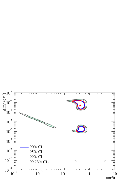
Figure 1: SNO-only neutrino oscillation contours, including pure $D_{2}O$ day/night spectra, salt CC, NC, ES fluxes, with ${}^{8}B$ flux free and hep flux fixed. The best-fit point is $\Delta m^{2}=4.7\times 10^{-5}$, $\tan^{2}\theta=0.43$, $f_{B}=1.03$, with $\chi^{2}$/d.o.f.=26.2/34. The inside of the covariance regions is allowed.

The $\chi^{2}_{\rm{cov}}$ calculated above from the SNO NC, CC and ES fluxes is added to a global analysis which includes data from all the other solar neutrino experiments. Systematic errors that are correlated between different experiments, such as cross section uncertainties or uncertainties on the ${}^{8}B$, are accounted for by including the covariance terms between different experimental results. The effect of the ${}^{8}B$ spectral shape uncertainty is determined at each grid point in the oscillation plane.

The global analysis includes the Homestake results bib:cl , the updated Gallium flux measurements bib:lownu ; bib:nu2002 , the SK zenith spectra bib:sktime , and the $D_{2}O$ and salt results from SNO bib:snod2o ; bib:snoDN ; bib:snosalt . At each grid point in the $\Delta m^{2}-\tan^{2}\theta$ plane, the expected rate for each energy bin is calculated and compared to the measured rate. The free parameters in the global fit are the total ${}^{8}B$ flux, the difference of the squared masses $\Delta m^{2}$, and the mixing angle $\theta$. The higher energy $hep$ $\nu_{e}$ flux is fixed at $9.3\times 10^{3}$ cm^-2 s^-1. Contours are generated in $\Delta m^{2}$ and $\tan^{2}\theta$ for $\Delta\chi^{2}_{\rm{cov}}$ = 4.61 (90% CL), 5.99 (95% CL), 9.21 (99% CL), and 11.83 (99.73% CL). We assume a Gaussian distribution of $R_{n}^{\rm{exp}}$ for a given value of the true parameters $\delta m^{2}$ and $\tan^{2}\theta$ when we map the survival probability into the MSW plane bib:freq . As presented in Fig 2(a), the combined results of all solar neutrino experiments can be used to determine a unique region of the oscillation parameters; the allowed region in this parameter space shrinks considerably to a portion of the Large Mixing Angle (LMA) region.

A global analysis including the KamLAND reactor anti-neutrino results bib:kamland shrinks the allowed region further, with a best-fit point of $\Delta m^{2}=7.1^{+1.2}_{-0.6}\times 10^{-5}$ eV² and $\theta=32.5^{+2.4}_{-2.3}$ degrees, where the errors reflect $1\sigma$ constraints on the 2-dimensional region. This is summarized in Fig. 2(b). With the new SNO measurements, the allowed region is constrained to only the lower band of LMA at $>99\%$ CL. The best-fit point with a one dimensional projection of the uncertainties in the individual parameters (marginalized uncertainties) is $\Delta m^{2}=7.1^{+1.0}_{-0.3}\times 10^{-5}$ eV² and $\theta=32.5^{+1.7}_{-1.6}$ degrees. This disfavors maximal mixing at a confidence level equivalent to 5.4 standard deviations and indicates $\tan^{2}\theta<1$. In our interpretation, the $\chi^{2}_{\rm{cov}}$ for $\theta=45.0$ is $5.4^{2}$ higher than the best LMA fit. The solution $\tan^{2}\theta<1$ corresponds to the neutrino mass hierarchy $m_{2}>m_{1}$.

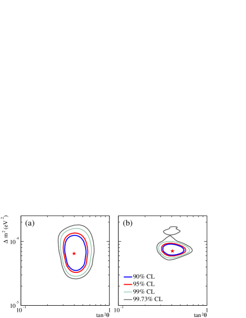
Figure 2: Allowed region of the $\Delta m^{2}-\tan^{2}\theta$ plane determined by a $\chi^{2}$ fit to (a) the Chlorine, Gallium, SK, and SNO experiments. The best-fit point is $\Delta m^{2}=6.5\times 10^{-5}$, $\tan^{2}\theta=0.40$, $f_{B}=1.04$, with $\chi^{2}$/d.o.f.=70.2/81. (b) Solar global + KamLAND. The best-fit point is $\Delta m^{2}=7.1\times 10^{-5}$, $\tan^{2}\theta=0.41$, $f_{B}=1.02$. The inside of the covariance contours is the allowed region.

VI Pull Analysis

The pull method allows a split of the residuals from the observables and the systematic uncertainties bib:fogli . This alternative approach embeds the effect of each independent $k^{\rm{th}}$ source of systematics through a shift of the difference $(R^{\rm{exp}}_{n}-R^{\rm{th}}_{n})$ by an amount $\epsilon_{k}c_{n}^{k}$. The normalization condition for the $K$ independent sources of systematic uncertainty is implemented through quadratic penalties in the global $\chi^{2}$, which is minimized with respect to all $\epsilon_{k}$’s

$$\chi^{2}_{\rm{pull}}=\sum_{n=1}^{N}\left(\frac{R_{n}^{\rm{exp}}-R_{n}^{\rm{th}}-\sum_{k=1}^{K}\epsilon_{k}c_{n}^{k}}{u_{n}}\right)^{2}+\sum_{k=1}^{K}\epsilon_{k}^{2}\,.$$ (15)

In an experimental context, the pull approach is not blind since it uses the data to constrain the systematic uncertainties. Systematic shifts calculated with the pull method should not be used as iterative corrections to experimental systematic uncertainties since it might lead to biases in the estimation of the mixing parameters. Nevertheless, the pull approach provides a nice framework to study each component of a global fit after a detailed study of the systematic uncertainty of each observables. See details in Ref. bib:fogli .

VII Summary

A summary of how to use the new salt data published by SNO is described in the context of solar neutrino analyses of matter-enhanced oscillation of two active flavors. Solar neutrino oscillation is clearly established by SNO. Matter effects bib:msw explain the energy dependence of solar oscillations with Large Mixing Angle (LMA) solutions favored. The global analysis of the solar and reactor neutrino results yields $\Delta m^{2}=7.1^{+1.0}_{-0.3}\times 10^{-5}$ eV² and $\theta=32.5^{+1.7}_{-1.6}$ degrees.

SNO is presently analyzing its full salt data set with a detailed treatment of the day/night and spectral information. In the future SNO will perform a global oscillation fit with a maximum-likelihood method.

- (1) Q.R. Ahmad et al., Submitted to Phys. Rev. Lett., Sept. 2003, nucl-ex/0309004.
- (2) J.N. Bahcall, H.M. Pinsonneault, and S. Basu, Astrophys. J. 555, 990 (2001).
- (3) Z. Maki, M. Nakagawa, S. Sakata, Prog. Theor. Phys. 28, 870 (1962); B. Pontecorvo, Sov. Phys. JETP 26, 984 (1968).
- (4) J. Boger et al., Nucl. Inst. Meth. A 449, 172 (2000).
- (5) C.E. Ortiz et al., Phys. Rev. Lett. 85, 2909 (2000).
- (6) Q.R. Ahmad et al., Phys. Rev. Lett. 89, 011301 (2002).
- (7) Q.R. Ahmad et al., Phys. Rev. Lett. 89, 011302 (2002).
- (8) B.T. Cleveland et al., Ap. J. 496, 505 (1998).
- (9) V. Gavrin, 4th International Workshop on Low Energy and Solar Neutrinos, Paris, May 2003.
- (10) T. Kirsten, XXth Int. Conf. on Neutrino Phy Astrophysics, Munich, May 2002; Nucl. Phys. B (Proc. Suppl.) 118 (2003).
- (11) S. Fukuda et al., Phys. Rev. Lett. 86, 5651 (2001); S. Fukuda et al., Phys. Lett. B 539, 179 (2002).
- (12) P. Creminelli, G. Signorelli, and A. Strumia, JHEP 05, 052 (2001).
- (13) K. Eguchi et al., Phys. Rev. Lett. 90, 021802 (2003).
- (14) G.L. Fogli, E. Lisi, A. Marrone, D. Montanino, and A. Palazz, Phys. Rev. D 66, 053010 (2002).
- (15) S.P. Mikheyev and A.Yu. Smirnov, Sov. J. Nucl. Phys. 42, 913 (1985); L. Wolfenstein, Phys. Rev. D 17, 2369 (1978).