New Measurements of the $D_{s}^{+}\rightarrow\phi\;\mu^{+}\nu$ Form Factor Ratios

Abstract

Using a large sample of $D_{s}^{+}\rightarrow\phi\;\mu^{+}\nu$ decays collected by the FOCUS photoproduction experiment at Fermilab, we present new measurements of two semileptonic form factor ratios: $r_{v}$ and $r_{2}$. We find $r_{v}=1.549\pm 0.250\pm 0.145{}$ and $r_{2}=0.713\pm 0.202\pm 0.266{}$. These values are consistent with $r_{v}$ and $r_{2}$ form factors measured for the process $D^{+}\rightarrow\overline{K}^{*0}\ell^{+}\nu_{\ell}$.

See http://www-focus.fnal.gov/authors.html for additional author information

1 Introduction

This paper provides new measurements of the parameters that describe $D_{s}^{+}\rightarrow\phi\;\mu^{+}\nu$ decay. The $D_{s}^{+}\rightarrow\phi\;\mu^{+}\nu$ decay amplitude is described [1] by four form factors with an assumed (pole form) $q^{2}$ dependence. Following earlier experimental work  [2, 3, 4, 5, 6, 7, 8, 9, 10, 11, 12, 13], the $D_{s}^{+}\rightarrow\phi\;\mu^{+}\nu$ amplitude is then described by ratios of form factors taken at $q^{2}$ = 0. The traditional set is: $r_{2}$, $r_{3}$, and $r_{v}$ which we define explicitly after Equation 8. According to flavor SU(3) symmetry, one expects that the the form factor ratios describing $D_{s}^{+}\rightarrow\phi\;\mu^{+}\nu$ should be close to those describing $D^{+}\rightarrow\overline{K}^{*0}\mu^{+}\nu$ since the $D_{s}^{+}$ only differs from the $D^{+}$ through the replacement of a $\overline{d}$ quark by a $\overline{s}$ quark spectator. The existing lattice gauge calculations [14] predict that the form factor ratios describing $D_{s}^{+}\rightarrow\phi\;\ell^{+}\nu_{\ell}$ should lie within 10% of those describing $D^{+}\rightarrow\overline{K}^{*0}\ell^{+}\nu_{\ell}$. Although the measured $r_{v}$ form factors are quite consistent between $D_{s}^{+}\rightarrow\phi\;\ell^{+}\nu_{\ell}$ and $D^{+}\rightarrow\overline{K}^{*0}\ell^{+}\nu_{\ell}$, there is presently a 3.3 $\sigma$ discrepancy between the $r_{2}$ values measured for these two processes with the previously measured $D_{s}^{+}\rightarrow\phi\;\ell^{+}\nu_{\ell}$ value being a factor of about 1.8 times larger than the $r_{2}$ value measured for $D^{+}\rightarrow\overline{K}^{*0}\ell^{+}\nu_{\ell}$ [7]. One quark model calculation [15] offers a possible explanation for the apparent inconsistency in the $r_{2}$ values measured for $D^{+}\rightarrow\overline{K}^{*0}\ell^{+}\nu_{\ell}$ and $D_{s}^{+}\rightarrow\phi\;\ell^{+}\nu_{\ell}$.

Five kinematic variables that uniquely describe $D_{s}^{+}\rightarrow K^{+}K^{-}\mu^{+}\nu$ decay are illustrated in Figure 1. These are the $K^{-}K^{+}$ invariant mass ($m_{K^{+}K^{-}}$) , the square of the $\mu\nu$ mass ($q^{2}$), and three decay angles: the angle between the $K^{+}$ and the $D_{s}^{+}$ direction in the $K^{-}K^{+}$ rest frame ($\theta_{\textrm{v}}$), the angle between the $\nu$ and the $D_{s}^{+}$ direction in the $\mu\nu$ rest frame ($\theta_{\ell}$), and the acoplanarity angle between the two decay planes ($\chi$). These angular conventions on $\theta_{\ell}$ and $\theta_{\textrm{v}}$ apply to both the $D_{s}^{+}$ and $D_{s}^{-}$. The sense of the acoplanarity variable is defined via a cross product expression of the form: $(\vec{P}_{\mu}\times\vec{P}_{\nu})\times(\vec{P}_{K^{-}}\times\vec{P}_{K^{+}})\cdot\vec{P}_{{K^{-}}{K^{+}}}$ where all momentum vectors are in the $D_{s}^{+}$ rest frame. Since this expression involves five momentum vectors, as one goes from $D_{s}^{+}\rightarrow D_{s}^{-}$ one must change $\chi\rightarrow-\chi$ in Equation 8 to get the same intensity for the $D_{s}^{+}$ and $D_{s}^{-}$ assuming CP symmetry.

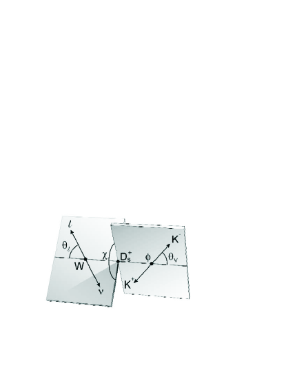
Figure 1: Definition of kinematic variables.

Using the notation of [1], we write the decay distribution for $D_{s}^{+}\rightarrow\phi\;\mu^{+}\nu$ in terms of the four helicity basis form factors: $H_{+}~{},~{}H_{0}~{},~{}H_{-}~{},H_{t}$.

$${d^{5}\Gamma\over dm_{K\pi}~{}dq^{2}~{}d\cos\theta_{\textrm{v}}~{}d\cos\theta_{\ell}~{}d\chi}\propto K(q^{2}{}-m_{l}^{2})\left\{\left|\begin{array}[]{l}(1+\cos\theta_{\ell})\sin\theta_{\textrm{v}}e^{i\chi}\textrm{B}_{\phi}H_{+}\\ -\,(1-\cos\theta_{\ell})\sin\theta_{\textrm{v}}e^{-i\chi}\textrm{B}_{\phi}H_{-}\\ -\,2\sin\theta_{\ell}(\cos\theta_{\textrm{v}}\textrm{B}_{\phi}+Ae^{i\delta})H_{0}\\ \end{array}\right|^{2}\right.$$ (4)

$$+\frac{m^{2}_{\ell}}{q^{2}}\left.\left|\begin{array}[]{l}\sin\theta_{\ell}\sin\theta_{\textrm{v}}\textrm{B}_{\phi}\left(e^{i\chi}H_{+}+e^{-i\chi}H_{-}\right)\\ +\,2\cos\theta_{\ell}\left(\cos\theta_{\textrm{v}}\textrm{B}_{\phi}+Ae^{i\delta}\right)H_{0}\\ +\,2\left(cos\theta_{\textrm{v}}\textrm{B}_{\phi}+Ae^{i\delta}\right)H_{t}\end{array}\right|^{2}\right\}\phantom{xxx}$$ (8)

where $K$ is the momentum of the $K^{-}K^{+}$ system in the rest frame of the $D_{s}^{+}$. The first term gives the intensity for the $\mu^{+}$ to be right-handed, while the (highly suppressed) second term gives the intensity for it to be left-handed. The helicity basis form factors are given by:

$$H_{\pm}(q^{2}) = (M_{D}+m_{K\pi})A_{1}(q^{2})\mp 2{M_{D}K\over M_{D}+m_{K\pi}}V(q^{2})$$

$$H_{0}(q^{2}) = {1\over 2m_{K\pi}\sqrt{q^{2}}}\left[(M^{2}_{D}-m^{2}_{K\pi}-q^{2})(M_{D}+m_{K\pi})A_{1}(q^{2})-4{M^{2}_{D}K^{2}\over M_{D}+m_{K\pi}}A_{2}(q^{2})\right]$$

$$H_{t}(q^{2}) = {M_{D}K\over M_{K\pi}\sqrt{q^{2}}}\left[(M_{D}+M_{K\pi})A_{1}(q^{2})-{(M^{2}_{D}-M^{2}_{K\pi}+q^{2})\over M_{D}+M_{K\pi}}A_{2}(q^{2})+{2q^{2}\over M_{D}+M_{K\pi}}A_{3}(q^{2})\right]$$

The vector and axial form factors are generally parameterized by a pole dominance form:

$$A_{i}(q^{2})={A_{i}(0)\over 1-q^{2}/M_{A}^{2}}~{}~{}~{}~{}~{}~{}~{}~{}V(q^{2})={V(0)\over 1-q^{2}/M_{V}^{2}}$$

where we use nominal (spectroscopic) pole masses of $M_{A}=2.5~{}\textrm{GeV}/c^{2}$ and $M_{V}=2.1~{}\textrm{GeV}/c^{2}$. The $\textrm{B}_{\phi}$ denotes the Breit-Wigner amplitude describing the $\phi$ resonance:

$$\textrm{B}_{\phi}=\frac{\sqrt{m_{0}\Gamma\,}\left(\frac{P^{*}}{P_{0}^{*}}\right)}{m_{KK}^{2}-m_{0}^{2}+im_{0}\Gamma\left(\frac{P^{*}}{P_{0}^{*}}\right)^{3}}$$

Equation 8 includes a possible $s$-wave amplitude coupling to the virtual $W^{+}$ with the same $q^{2}$ dependence as that of the $H_{0}$ (or $H_{t}$) form factor. Evidence for such an $s$-wave amplitude term for the decay $D^{+}\rightarrow K^{-}\pi^{+}\mu^{+}\nu$ was presented in Reference [3]. An explicit search was made for $s$-wave amplitude interference with the process $D_{s}^{+}\rightarrow\phi\;\mu^{+}\nu$ and no evidence for this interference was seen. We were able to limit the $s$-wave contribution to be less than 5% of the maximum of the $\phi$ Breit-Wigner peak in the $H_{0}$ piece of Equation 8 at the 90% confidence level. The results presented here will therefore assume $A=0$ in Equation 8. Under these assumptions, the decay intensity is then parameterized by the $r_{v}{}\equiv V(0)/A_{1}(0)~{},~{}r_{2}{}\equiv A_{2}(0)/A_{1}(0)~{},~{}r_{3}{}\equiv A_{3}(0)/A_{1}(0)$ form factor ratios describing the $D_{s}^{+}\rightarrow\phi\;\mu^{+}\nu$ amplitude. Throughout this paper, unless explicitly stated otherwise, the charge conjugate is also implied when a decay mode of a specific charge is stated.

2 Experimental and analysis details

The data for this paper were collected in the Wideband photoproduction experiment FOCUS during the Fermilab 1996–1997 fixed-target run. In FOCUS, a forward multi-particle spectrometer is used to measure the interactions of high energy photons on a segmented BeO target. The FOCUS detector is a large aperture, fixed-target spectrometer with excellent vertexing and particle identification. Most of the FOCUS experiment and analysis techniques have been described previously [3, 16, 17, 18, 20]. Our analysis cuts were chosen to give reasonably uniform acceptance over the five kinematic decay variables, while maintaining a strong rejection of backgrounds. To suppress background from the re-interaction of particles in the target region which can mimic a decay vertex, we required that the charm secondary vertex was located at least three standard deviation outside of all solid material including our target and target microstrip system.

To isolate the $D_{s}^{+}\rightarrow\phi\;\mu^{+}\nu$ topology, we required that candidate muon, pion, and kaon tracks appeared in a secondary vertex with a confidence level exceeding 1%. The muon track, when extrapolated to the shielded muon arrays, was required to match muon hits with a confidence level exceeding 5%. The kaon was required to have a Čerenkov light pattern more consistent with that for a kaon than that for a pion by 1 unit of log likelihood [18]. To further reduce non-charm background we required that our primary vertex consisted of at least two charged tracks. To further reduce muon misidentification, a muon candidate was allowed to have at most one missing hit in the 6 planes comprising our inner muon system and an energy exceeding 10 GeV. In order to suppress muons from pions and kaons decaying within our apparatus, we required that each muon candidate had a confidence level exceeding 1% to the hypothesis that it had a consistent trajectory through our two analysis magnets.

Non-charm and random combinatoric backgrounds were reduced by requiring both a detachment between the vertex containing the $K^{-}K^{+}\mu^{+}$ and the primary production vertex of at least 5 standard deviations.

Possible background from $D^{+}\rightarrow K^{-}K^{+}\pi^{+}$, where a pion is misidentified as a muon, was reduced by treating the muon as a pion and requiring the reconstructed $KK\pi$ mass be less than $1.8~{}\textrm{GeV}/c^{2}{}$. The $m_{K^{+}K^{-}}$ distribution for our $D_{s}^{+}\rightarrow K^{+}K^{-}\mu^{+}\nu$ candidates is shown in Figure 2.

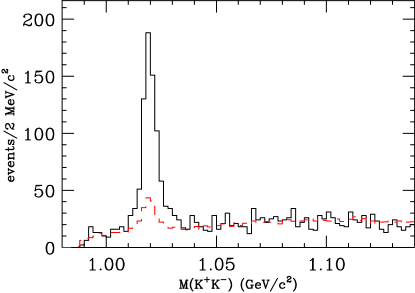
Figure 2: The data is the solid histogram and ccbar background Monte Carlo is the dashed histogram. The ccbar background Monte Carlo is normalized to the same number of events in the sideband region $1.040~{}\textrm{GeV}/c^{2}{}<m_{K^{+}K^{-}}{}<1.14~{}\textrm{GeV}/c^{2}$.

The technique used to reconstruct the neutrino momentum through the $D_{s}^{+}$ line-of-flight, and tests of our ability to simulate the resolution on kinematic variables that rely on the neutrino momentum are described in Reference [3].

3 Fitting Technique

The $r_{v}$ and $r_{2}$ form factors were fit to the probability density function described by four fitted kinematic variables ($q^{2}$, $\cos\theta_{\textrm{v}}$, $\cos\theta_{\ell}$, and $\chi$) for decays in the mass range $1.010<m_{K^{+}K^{-}}{}<1.030$. We use a variant of the continuous fitting technique developed by the E691 Collaboration [19] for fitting decay intensities where several of the kinematic variables have very poor resolution such as the four variables that rely on reconstructed neutrino kinematics.

The fit which determines the $r_{v}$ and $r_{2}$ form factor ratios minimizes the sum of $w=-2\ln{I}$ where $I$ is the normalized decay intensity at each datum. The intensity at each datum is estimated by the weight of Monte Carlo events that lie within a small window of each of the four (reconstructed) kinematic variables of the given datum. Some care is needed in choosing a reasonable size of the windows since too small a window will result in fluctuations due to finite Monte Carlo statistics, and too large a window will create a bias in the result. Our principal tool in deciding a reasonable window was to check for biases and fluctuations outside of reported statistical errors using a Monte Carlo simulation that included charm backgrounds with $r_{v}$ and $r_{2}$ values very close to the result reported here. Variations in the final results due to the window choice were included in the estimate of the systematic error.

Two Monte Carlos were employed: a weighted $D_{s}^{+}\rightarrow\phi\;\mu^{+}\nu$ signal Monte Carlo that was generated flat in the four fitted kinematic variables ($q^{2}$, $\cos\theta_{\textrm{v}}$, $\cos\theta_{\ell}$, and $\chi$) and an unweighted background Monte Carlo which simulated all known charm decays (apart from the $D_{s}^{+}\rightarrow\phi\;\mu^{+}\nu$ signal) as well as our misidentification levels. The intensity about each datum is an appropriate average of the weighted signal MC and the unweighted background Monte Carlo. The averaging depended on the background fraction determined by matching the number of events in the $\phi$ sideband region $1.040<m_{K^{+}K^{-}}{}<1.14~{}\textrm{GeV}/c^{2}{}$ in the background Monte Carlo to the sideband level observed in the data.

Our fit was to the $r_{v}$ and $r_{2}$ form factor ratios with $r_{3}{}$ and the possible $s$-wave amplitude set to zero. We decided not to fit for the $r_{3}$ form factor ratio since our anticipated $r_{3}$ error given our sample size would be too large to be meaningful.

Figure 3 compares the data and model for projections of $\cos\theta_{\textrm{v}}$, $\cos\theta_{\ell}$, $\chi$ and $q^{2}{}/q^{2}_{\rm max}$. Most of these distributions follow the predicted values reasonably well. A slight discrepancy is evident in the low $q^{2}{}/q^{2}_{\rm max}$ projection (below $q^{2}{}/q^{2}_{\rm max}{}<0.2~{}$). A stronger effect was observed in Reference [2] possibly owing to our much larger yield in the $D^{+}\rightarrow K^{-}\pi^{+}\mu^{+}\nu$ final state.

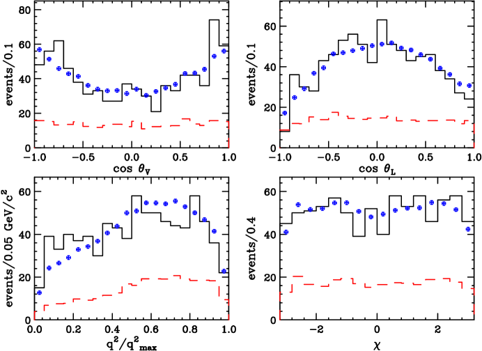
Figure 3: The data are given by the upper histogram. The model (crosses with flats) includes the signal computed with the fitted form factor ratios plus the sideband normalized ccbar background. The lower histogram (dashed) shows the projections of the ccbar background. (a) $\cos\theta_{\textrm{v}}$ (b) $\cos\theta_{\ell}$ (c) $q^{2}{}/q^{2}_{\rm max}$ (d) $\chi$

Figure 4 compares the $\cos\theta_{\textrm{v}}$ and $\cos\theta_{\ell}$ distribution between the data and our Monte Carlo model for events at high and low $q^{2}$. As $q^{2}{}\rightarrow q^{2}{}_{\rm max}$ one expects an isotropic distribution in both $\cos\theta_{\textrm{v}}$ and $\cos\theta_{\ell}$ since all three helicity basis form factors become equal. The data presented in Figure 4 match this expectation relatively well.

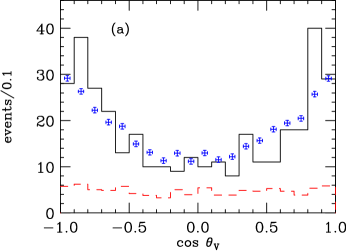
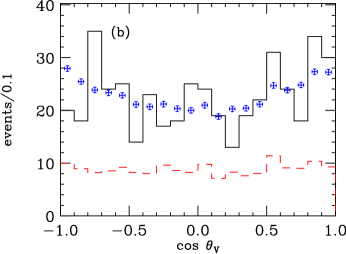
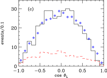
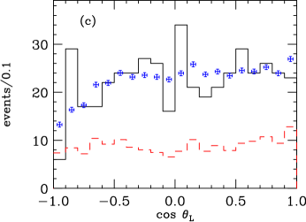
Figure 4: Various $\cos\theta_{\textrm{v}}$ and $\cos\theta_{\ell}$ projections. The data are given by the upper histogram. The model (crosses with flats) includes the signal computed with the fitted form factor ratios plus the sideband normalized ccbar background. The lower histogram (dashed) shows the projections of the ccbar background. (a) The $\cos\theta_{\textrm{v}}$ distribution for $q^{2}$/$q^{2}{}_{\rm max}<0.5$ (b) The $\cos\theta_{\textrm{v}}$ distribution for $q^{2}$/$q^{2}{}_{\rm max}>0.5$ (c) The $\cos\theta_{\ell}$ distribution for $q^{2}$/$q^{2}{}_{\rm max}<0.5$ (d) The $\cos\theta_{\ell}$ distribution for $q^{2}$/$q^{2}{}_{\rm max}>0.5$

4 Form Factor Ratio Systematic Errors

Three basic approaches were used to determine the systematic error on the form factor ratios. In the first approach, we measured the stability of the branching ratio with respect to variations in analysis cuts designed to suppress backgrounds. In these studies we varied cuts such as the detachment criteria, particle identification cuts, vertex isolation cuts, and the out-of-material cut. Sixteen such cut sets were considered. In the second approach, we split our sample according to a variety of criteria deemed relevant to our acceptance, production, and decay models and estimated a systematic based on the consistency of the form factor ratio measurements among the split samples. These included computing separate form factors for particles and antiparticles, and comparing the values obtained over the full data set to values obtained from a subset (2/3) of the data in which the target silicon [20] was operational. In the third approach we checked the stability of the branching fraction as we varied specific parameters in our Monte Carlo model and fitting procedure. These included varying the level of the charm background and in the size of the kinematic windows used to associate Monte Carlo events with data points in the computation of the fitting intensity. The only non-neglible systematic error was that due to variation in the results over the sixteen cut selections. Combining all three non-zero systematic error estimates in quadrature we find $r_{v}=1.549\pm 0.250\pm 0.145{}$ and $r_{2}=0.713\pm 0.202\pm 0.266{}$.

5 Summary

In Table 1 we compare our results to other experiments. Our weighted average of all the experimental results is $r_{v}=1.678\pm 0.213$ and $r_{2}=1.292\pm 0.194$ where systematic errors have been included. We obtain a confidence level of 44.3% that all 5 experiments have a consistent $r_{v}$ and a confidence level of 21.5 % that all $r_{2}$ measurements are consistent. Figure 5 is a graphical representation of Table 1.

Table 1: Measurements of the $D_{s}^{+}\rightarrow\phi\;\mu^{+}\nu$ form factor ratios

Group	$r_{v}$	$r_{2}$
This work	$1.549\pm 0.250\pm 0.145$	$0.713\pm 0.202\pm 0.266$
E791[7]	$2.27\pm 0.35\pm 0.22$	$1.570\pm 0.250\pm 0.190$
CLEO[8]	$0.9\pm 0.6\pm 0.3$	$1.400\pm 0.500\pm 0.300$
E653[12]	$2.3\pm 1.0\pm 0.4$	$2.100\pm 0.550\pm 0.200$
E687[10]	$1.8\pm 0.9\pm 0.2$	$1.100\pm 0.800\pm 0.100$

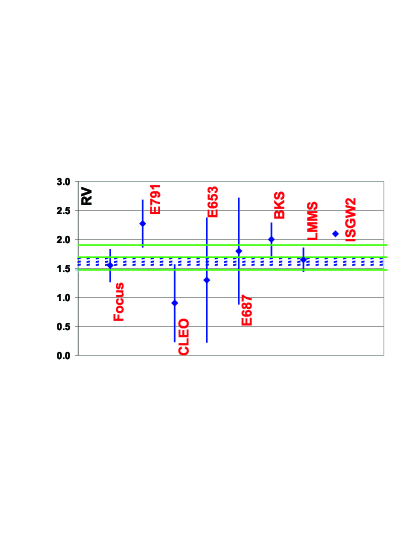
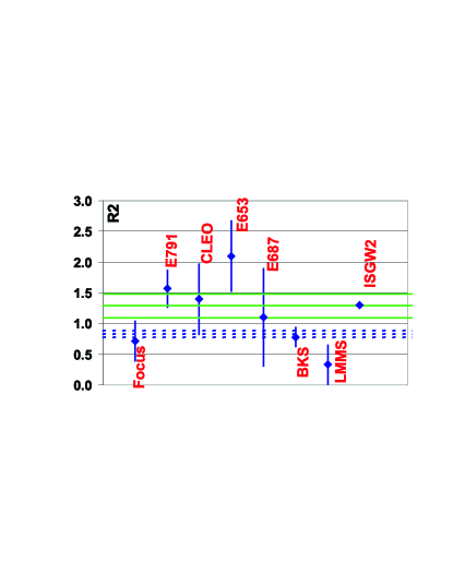
Figure 5: Comparision to previous data and calculations of the $D_{s}^{+}\rightarrow\phi\;\mu^{+}\nu$ form factors. The three solid green lines represent the weighted average of the world’s experimental data for $D_{s}^{+}\rightarrow\phi\;\mu^{+}\nu$ and $\pm 1~{}\sigma$. The three dashed blue lines represent the weighted average of the world’s experimental data on $D^{+}\rightarrow\overline{K}^{*0}\mu^{+}\nu$ and $\pm 1~{}\sigma$.

Our measured $r_{v}$ and $r_{2}$ values for $D_{s}^{+}\rightarrow\phi\;\mu^{+}\nu$ are very consistent with our measured $r_{v}$ and $r_{2}$ values for $D^{+}\rightarrow\overline{K}^{*0}\mu^{+}\nu$ [2]. The measurements reported here call into question the apparent inconsistency between $r_{2}$ values the $D^{+}\rightarrow\overline{K}^{*0}\ell^{+}\nu_{\ell}$ and $D_{s}^{+}\rightarrow\phi\;\ell^{+}\nu_{\ell}$ form factors present in previously published data and are consistent with the theoretical expectation that the form factors for the two processes should be very similar.

6 Acknowlegments

We wish to acknowledge the assistance of the staffs of Fermi National Accelerator Laboratory, the INFN of Italy, and the physics departments of the collaborating institutions. This research was supported in part by the U. S. National Science Foundation, the U. S. Department of Energy, the Italian Istituto Nazionale di Fisica Nucleare and Ministero dell’Università e della Ricerca Scientifica e Tecnologica, the Brazilian Conselho Nacional de Desenvolvimento Científico e Tecnológico, CONACyT-México, the Korean Ministry of Education, and the Korean Science and Engineering Foundation.

References

[1]
J.G. Korner and G.A. Schuler, Z. Phys. C 46 (1990) 93.
[2]
FOCUS Collab., J.M. Link et al., Phys. Lett. B 544 (2002) 89.
[3]
FOCUS Collab., J.M. Link et al., Phys. Lett. B 535 (2002) 43.
[4] BEATRICE Collab., M. Adamovich et al., Eur. Phys. J. C 6 (1999) 35.
[5] E791 Collab., E. M. Aitala et al., Phys. Rev. Lett. 80 (1998) 1393.
[6] E791 Collab., E. M. Aitala et al., Phys. Lett. B 440 (1998) 435.
[7]
E791 Collab. E.M. Aitala et al., Phys. Lett. B 450 (1999) 294.
[8]
CLEO Collab. P. Avery et al., Phys. Lett. B 337 (1994) 405.
[9] E687 Collab., P.L. Frabetti et al., Phys. Lett. B 307 (1993) 262.
[10]
E687 Collab. P. L. Frabetti et al., Phys. Lett. B 328 (1994) 187.
[11] E653 Collab., K. Kodama et al., Phys. Lett. B 274 (1992) 246.
[12]
E653 Collab. K. Kodama et al., Phys. Lett. B 309 (1993) 483.
[13] E691 Collab., J. C. Anjos et al., Phys. Rev. Lett. 65 (1990) 2630.
[14]
C. W. Benard, A. X. El-Khadra, and A. Soni, Phys. Rev. D45 (1992) 869.
V. Lubicz,G. Martinelli, M. S. McCarthy, and C. T. Sachrajda, Phys. Lett. B 274 (1992) 415.
[15]
D. Scora and N. Isgur, Phys. Rev. D 52 (1995) 2783.
[16] E687 Collab., P. L. Frabetti et al.,
Nucl. Instrum. Methods A 320 (1992) 519.
[17]FOCUS Collab., J. M. Link et al., Phys. Lett. B 485 (2000) 62.
[18]FOCUS Collab., J. M. Link et al., Nucl. Instrum. Methods A 484
(2002) 270.
[19]D.M. Schmidt, R.J. Morrision, and M.S. Witherell,
Nucl. Instrum. Methods. A 328 (1993) 547.
[20]
FOCUS Collab., J. M. Link et al.,
Nucl. Instrum. Methods A 516 (2003) 364.