Global Fits of the CKM Matrix

Abstract

We report upon the present status of global fits to Cabibbo-Kobayashi-Maskawa matrix.

1 Introduction

The three-family Cabibbo-Kobayashi-Maskawa (CKM) quark-mixing matrix is a key element of the Standard Model (SM). The nine complex CKM elements are completely specified by three mixing angles and one phase that is responsible for $C\!P$ violation in the SM. Measuring the CKM matrix elements in various ways provides consistency tests of the matrix elements itself and with unitarity. Any significant inconsistency with the SM would indicate the presence of new physics.

A convenient parameterization of the CKM matrix is the Wolfenstein approximation bib:wolfenstein , which to order $O(\lambda^{3})$ is given by:

$$V=\pmatrix{1-{\lambda^{2}\over 2}&\lambda&A\lambda^{3}(\rho-i\eta)\cr-\lambda&1-{\lambda^{2}\over 2}&A\lambda^{2}\cr A\lambda^{3}(1-\bar{\rho}-i\bar{\eta})&-A\lambda^{2}&1\cr}+O(\lambda^{4}),$$ (1)

where $\lambda=0.2241\pm 0.0033$ is the best-known parameter measured in semileptonic $K$ decays, $A=0.82$ is determined from semileptonic $B$ decays to charmed particles with an accuracy of $\simeq 6\%$ and $\bar{\rho}=\rho\cdot(1-\lambda^{2}/2)$ and $\bar{\eta}=\eta\cdot(1-\lambda^{2}/2)$ are least-known.

The unitarity of the CKM matrix yields six triangular relations of which $V_{ud}V^{*}_{ub}+V_{cd}V^{*}_{cb}+V_{td}V^{*}_{tb}=0$ is well-suited for experimental tests. In order to determine the apex of the unitarity triangle $(\bar{\rho},\bar{\eta})$ presently eight measurements are used as input, the $B$ semileptonic branching fractions ${\cal B}(B\rightarrow X_{c}\ell\nu)$, ${\cal B}(B\rightarrow X_{u}\ell\nu)$, and ${\cal B}(B\rightarrow\rho\ell\nu)$, the normalized $B\rightarrow D^{*}\ell\nu$ rate at zero recoil, ${\cal F}(1)|V_{ub}|^{2}$, the $B^{0}_{d}$ and $B^{0}_{s}$ oscillations frequencies $\Delta m_{B_{d}}$ and $\Delta m_{B_{s}}$, the parameter $|\epsilon_{K}|$ that specifies $C\!P$ violation in the $K^{0}\bar{K}^{0}$ system, as well as $\sin 2\beta$ which is measured in $C\!P$ asymmetries of charmonium $K^{0}_{S}\ (K^{0}_{L})$ final states. Though many of these measurements themselves are rather precise their translation to the $\bar{\rho}-\bar{\eta}$ plane is affected by large non-gaussian theoretical uncertainties. Various approaches, which treat theoretical errors in different ways, can be found in the literature [2,3,4,5,6].

2 The Scan Method

The scan method is an unbiased procedure for extracting $A,\bar{\rho},\bar{\eta}$ from measurements. We select observables that allow us to factorize their predictions in terms of theoretical quantities $T_{i}$ that have an a priori unknown (and likely non-gaussian) error distribution $(\Delta_{i})$, other observables, and the CKM dependence expressed as functions of Wolfenstein parameters. As an example, consider the charmless semileptonic branching fraction for $B\rightarrow\rho\ell\nu$, which is predicted to be ${\cal B}(B\to\rho\ell\nu)=|V_{ub}|^{2}\cdot\widetilde{\Gamma}_{\rho\ell\nu}\cdot\tau_{B}$, where $\tau_{B^{0}}$ is the $B^{0}$ lifetime and $\widetilde{\Gamma}_{\rho\ell\nu}$ is the reduced rate affected by non-gaussian uncertainties. This analysis treats eleven theoretical parameters with non-gaussian errors, the reduced inclusive semileptonic rates $\widetilde{\Gamma}_{X_{u}\ell\nu}$ and $\widetilde{\Gamma}_{X_{c}\ell\nu}$, the form factor for $B\rightarrow D^{*}\ell\nu$ at zero recoil, ${\cal F}_{D^{*}}(1)$, the bag factors of the $K^{0}$ and $B^{0}$ systems, $B_{K}$ and$B_{B}$, the $B^{0}$ decay constant $f_{B}$, $\xi^{2}=f^{2}_{B_{s}}/f^{2}_{B_{d}}B_{B_{s}}/B_{B_{d}}$ and the QCD parameters $\eta_{1},\eta_{2},\eta_{3}$ and $\eta_{B}$.

We perform a $\chi^{2}$ minimization based on a frequentist approach by selecting a specific value for each $T_{i}$ within the allowed range (called a model). We perform individual fits for many models scanning over the allowed non-gaussian ranges of the $T_{i}$ parameter space. The QCD parameters are not scanned; their small errors are treated in the $\chi^{2}$ as gaussian. For theoretical quantities calculated on the lattice, which have gaussian errors ($B_{K}$, $B_{B}$, $f_{B}$ and $\xi$) we add specific $\chi^{2}$ terms. To account for correlations between observables that occur in more than one prediction, such as the masses of the $t$-quark, $c$-quark, and $W$-boson, $B$ hadron lifetimes, $B$ hadron production fractions and $\lambda$, we include additional terms in the $\chi^{2}$ function.

We consider a model to be consistent with the data if the fit probability yields $P(\chi^{2})>5\%$. We determine the best estimate for each of the 17 fit parameters and plot a $95\%$ confidence level (C.L.) contour in the $\bar{\rho}-\bar{\eta}$ plane. We overlay the $\bar{\rho}-\bar{\eta}$ contours of all accepted fits. In order to study correlations among the $T_{i}$ and constraints the data impose we perform global fits with non-gaussian theory errors scanned over a $\pm 5\Delta$ wide range (see section 5).

2.1 Treatment of $\Delta m_{B_{s}}$

Since $B^{0}_{s}\bar{B}^{0}_{s}$ oscillations have not been observed yet, a lower limit on $\Delta m_{B_{S}}$ at 95% C.L. has been determined by combining analyses of different experiments using the amplitude method bib:moser . To incorporate $\Delta m_{B_{S}}$ into the $\chi^{2}$ function, we use a new approach that is based upon the significance of a $\Delta m_{B_{s}}$ measurement bib:cern :

$$S=\sqrt{{N\over 2}}f_{B_{s}}(1-2w)e^{-{1\over 2}(\Delta m_{s}\sigma_{t})^{2}},$$ (2)

where $N$ is the sample size, $f_{B_{s}}$ is the $B_{s}$ purity, $w$ is the mistag fraction, and $\sigma_{t}$ is the resolution. Substituting $C$ for $\sqrt{{N\over 2}}f_{B_{s}}(1-2w)$ and interpreting $S$ as the number of standard deviations by which $\Delta m_{B_{s}}$ differs from zero, $S=\Delta m_{B_{s}}/\sigma_{\Delta{m_{B_{s}}}}$, we may define a contribution to the $\chi^{2}$ from the $\Delta m_{B_{s}}$ measurements as:

$$\chi^{2}_{\Delta{m_{B_{s}}}}=C^{2}\left(1-{\Delta\over\Delta{m_{B_{s}}}}\right)^{2}e^{-(\Delta{m_{B_{s}}}\sigma_{t})^{2}},$$ (3)

where $\Delta$ is the best estimate according to experiment. The values of $(\Delta,C^{2},\sigma_{t})$ are chosen to give a minimum at $17~{}\rm ps^{-1}$, and a $P(\chi^{2})=5\%$ at $\Delta{m_{B_{s}}}=14.4~{}\rm ps^{-1}$. In the region of small $\chi^{2}$, this function exhibits similar general features as that used in our previous global fits bib:eps , while it does not suffer from numerical instabilities arising from multiple minima. The two functions deviate at large values of $\chi^{2}$, where in any case poor fits result.

Table 1: Measurement inputs used in $\chi^{2}$ minimization

Observable	Value	Comment
${\cal B}(B\rightarrow X_{u}\ell\nu)$	$(2.03\pm 0.22_{exp}\pm 0.31_{th})\times 10^{-3}$	$\Upsilon(4S)$
${\cal B}(B\rightarrow X_{u}\ell\nu)$	$(1.71\pm 0.48_{exp}\pm 0.21_{th})\times 10^{-3}$	LEP
${\cal B}(B\rightarrow X_{c}\ell\nu)$	$0.1070\pm 0.0028$	$\Upsilon(4S)$
${\cal B}(B\rightarrow X_{c}\ell\nu)$	$0.1042\pm 0.0026$	LEP
${\cal B}(B\rightarrow\rho\ell\nu)$	$(2.68\pm 0.43_{exp}\pm 0.5_{th})\times 10^{-3}$	CLEO/BABAR
$|V_{cb}|F(1)$	$0.0388\pm 0.005\pm 0.009$	LEP/CLEO/Belle
$\Delta m_{B_{d}}$	$(0.503\pm 0.006)\rm ps^{-1}$	world average
$\Delta m_{B_{s}}$	$>14.4~{}\rm ps^{-1}@95\%C.L.$	LEP
$|\epsilon_{K}|$	$(2.271\pm 0.017)\times 10^{-3}$	PDG 2000 bib:groom
$\sin 2\beta$	$0.731\pm 0.055$	BABAR/Belle
$\lambda$	$0.2241\pm 0.0033$	world average

Figure 1: Results of the global fit in the $\bar{\rho}-\bar{\eta}$ plane.

Figure 2: Fit results in $\theta_{s}-\bar{\rho}$ plane from $a_{\phi K^{0}_{S}}$.

Table 2: Theoretical parameter with non-gaussian errors

$0.87\leq{\cal F}_{D^{*}}(1)\leq 0.95$	$38.0\leq\widetilde{\Gamma}(c\ell\nu)\leq 41.5~{}\rm ps^{-1}$
$12.0\leq\widetilde{\Gamma}(\rho\ell\nu)\leq 22.2~{}\rm ps^{-1}$	$54.8\leq\widetilde{\Gamma}(u\ell\nu)\leq 79.6~{}\rm ps^{-1}$
$0.72\leq B_{K}\leq 1.0$	$\sigma_{B_{K}}=0.06$ (gaussian)
$211\leq f_{B_{d}}\sqrt{B_{B_{d}}}\leq 235~{}\rm MeV$	$\sigma_{f_{B}\sqrt{B_{B}}}=33~{}\rm MeV$ (gaussian)
$1.18\leq\xi\leq 1.30$	$\sigma_{\xi}=0.04$ (gaussian)
$0.54\leq\eta_{B}\leq 0.56$	$1.0\leq\eta_{1}\leq 1.64$
$0.564\leq\eta_{2}\leq 0.584$	$0.43\leq\eta_{3}\leq 0.51$

Table 3: Results of $95\%$ C.L. range for $\bar{\rho},\bar{\eta},\alpha$ and $\gamma$ from the global fits shown in figure 1. For comparison results from RFIT and the Bayesian method are also given.

parameter	Scan method	RFIT bib:cern	Bayesian bib:cern
$\bar{\rho}$	-0.13 to 0.40	0.091 to 0.317	0.137-0.295
$\bar{\eta}$	0.22 to 0.48	0.273 to 0.408	0.295-0.409
$\alpha$	$50.4^{0}$ to $126.6^{0}$
$\gamma$	$34.4^{0}$ to $91.7^{0}$	$42.1^{0}$ to $75.7^{0}$	$47.0^{0}$ to $70.0^{0}$

3 Results of the global Fit

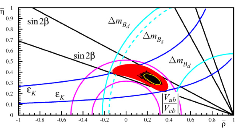
Figure 1 shows the result of scanning all $T_{i}$ simultaneously within $\pm 1\Delta$ of their allowed range except for the QCD parameters. We have used the input measurements summarized in table 1 and ranges for the $T_{i}$ listed in table 2. The black points represent the best estimates of $(\bar{\rho},\bar{\eta})$ for each model that is consistent with the data. The grey region shows the overlay of all corresponding $95\%\ \rm C.L.$ $\bar{\rho}-\bar{\eta}$ contours. For reference, the light ellipse depicts a typical contour. To guide the eye the $95\%\ \rm C.L.$ bounds on $|V_{ub}/V_{cb}|$, $|\epsilon_{K}|$, $\Delta m_{B_{d}}$ and $\sin 2\beta$ as well as the lower bound on $\Delta m_{B_{s}}$ are also plotted. From these fits we derive $95\%\ \rm C.L.$ ranges for $\bar{\rho},\bar{\eta},\alpha$ and $\gamma$ that are listed in table 3. For comparison, recent results from two other global fits (RFIT bib:ckmfitter , Bayesian fit bib:ciuchini ) are also shown.

Using the same source of inputs, several differences exist between the scan method and the other two approaches. First, we scan separately over the inputs of exclusive and inclusive $b\rightarrow u\ell\nu$ and $b\rightarrow c\ell\nu$ measurements. Second, we use a different approach to incorporate $\Delta m_{B_{s}}$. While in the Bayesian method theoretical quantities are parameterized in terms of gaussian and uniform distributions, we make no assumptions about their shape. Thus, the Bayesian fits tend to produce a smaller region in the $\bar{\rho}-\bar{\eta}$ plane and are more sensitive to fluctuations than corresponding fits in the scan method. In RFIT, the $\bar{\rho}-\bar{\eta}$ plane is scanned to find a solution in the theoretical parameter space. Since in RFIT a central region with equal likelihood is determined, it is not possible to give probabilities for individual points. In contrast, in the scan method individual contours have a statistical meaning, with the center point yielding the highest probability. Since the mapping of the theory parameters to the $\bar{\rho}-\bar{\eta}$ plane is not one-to-one, it is possible in the scan method to track which values of $(\bar{\rho},\bar{\eta})$ are preferred by the theory parameters.

4 Search for New Physics

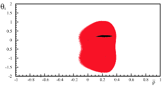
The decay $B\rightarrow\phi K^{0}_{S}$ that proceeds via a $b\rightarrow s\bar{s}s$ penguin loop is expected measure $\sin 2\beta$ in the SM to within $\sim\!4\%$. New physics contributions, however, may introduce a new phase $\theta_{s}$ that may change the $C\!P$ asymmetry $a_{\phi K^{0}_{S}}$ significantly from $a_{J/\psi K^{0}_{S}}$. The BABAR/Belle average of $S_{\phi K^{0}_{S}}=-0.39\pm 0.41$ has been updated this summer yielding $S_{\phi K^{0}_{S}}=-0.14\pm 0.33$ bib:hfag . The deviation from $\sin 2\beta$ has remained at $\sim 2.6\sigma$. In our global fit we introduce a new phase $\theta_{s}$. Figure 2 shows the overlay of all resulting contours in the $\theta_{s}-\bar{\rho}$ plane that have acceptable fit probabilities. Presently, the phase is consistent with zero as expected in the SM.

Physics beyond the SM may affect $B^{0}_{d}\bar{B}^{0}_{d}$ mixing and $C\!P$ violation in $B\rightarrow J/\psi K^{0}_{s}$ and $B\rightarrow\pi\pi$. Using a model-independent analysis bib:nir we can introduce a scale parameter, $r_{d}$, for $B^{0}_{d}\bar{B}^{0}_{d}$ mixing and an additional phase, $\theta_{d}$, for parameterizing $a_{\psi K^{0}_{s}}$. In the SM we expect $r_{d}=1$ and $\theta_{d}=0$. With present uncertainties $r_{d}$ and $\theta_{d}$ are consistent with the SM expectations (see bib:eps ).

Figure 3: Contours of the theory parameters $\widetilde{B}_{K}-\widetilde{V}_{ub}-\widetilde{V}_{cb}$ both resulting from inclusive reduced semileptonic rates for fit probabilities $P(\chi^{2})>32\%$ after scanning $\widetilde{B}_{K},\widetilde{f}_{B}\sqrt{B_{B}},\widetilde{\xi},\widetilde{\Gamma}(B\rightarrow X_{c}\ell\nu$ and $\widetilde{\Gamma}(B\rightarrow X_{u}\ell\nu$ over $\pm 5\Delta_{i}$ range.

5 Visualizing the role of theoretical errors

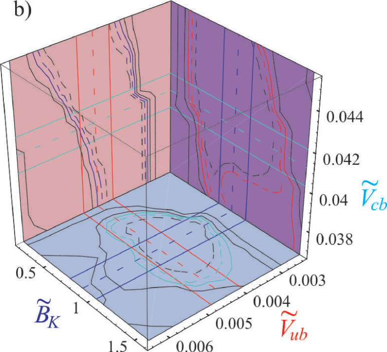
In addition to the global fits in the $\bar{\rho}-\bar{\eta}$ plane, we explore the impact of measurements on the theoretical parameters and their correlations. We typically scan theory parameters within $\pm 5\Delta$ and denote them with ^∼. Presently, we use either exclusive or inclusive $\widetilde{V}_{ub},\widetilde{V}_{cb}$ information and plot contours for three of the five scanned theoretical parameters for different conditions. An example is shown in Figure 3, where we have scanned inclusive $\widetilde{V}_{ub}$, inclusive $\widetilde{V}_{cb}$, $\widetilde{B}_{K}$, $\widetilde{f_{B_{d}}\sqrt{B_{B_{d}}}}$ and $\widetilde{\xi}$. For $\widetilde{V}_{ub}$, $\widetilde{V}_{cb}$ and $\widetilde{B}_{K}$ we plot two-dimensional contours on the surface of a cube. In each plane five contours are visible. The outermost contour (solid black) results from requiring a fit probability of $>32\%$. The next contour (also solid black) is obtained by restricting all other undisplayed theory parameters to their allowed range of $\pm 1\Delta$. The third solid line results by fixing the parameter orthogonal to plane to the allowed range, while the outer dashed line is found if the latter parameter is fixed to its central value. The internal dashed black line is obtained by fixing all undisplayed parameters to their central values. Further details, other combination plots and results for exclusive $\widetilde{V}_{ub}$ and $\widetilde{V}_{cb}$ scans are discussed in bib:eps .

6 Conclusion

The scan method provides a conservative, robust method that treats non-gaussian theoretical uncertainties in an unbiased way. This reduces conflicts with the SM resulting from unwarranted assumptions concerning the theoretical uncertainties, which is important in searches for new physics. The scan methods yields significantly larger ranges for the $\bar{\rho}-\bar{\eta}$ plane than the Bayesian method. Presently, all measurements are consistent with the SM expectation due to the large theoretical uncertainties. The deviation of $a_{\phi K^{0}_{s}}$ from $\sin 2\beta$ measured in charmonium $K^{0}_{S}\ (K^{0}_{L})$ modes is interesting but not yet significant. Model-independent parameterizations will become important in the future when theory errors are further reduced.

References

- (1) L. Wolfenstein, Phys. Rev. Lett. 51 (1983) 1945.
- (2) BABAR collaboration (P.F. Harrison and H.R. Quinn, eds.) SLAC-R-0504 (1998).
- (3) M. Ciuchini et al., J. High Energy Physics 107 (2001) 13.
- (4) A. Höcker et al., Eur. Phys. J. C 21 (2001) 225.
- (5) K. Schubert, CKM workshop Durham, April 5-9 (2003).
- (6) K. Hagiwara et al., Phys. Rev D 66 (2002) 010001.
- (7) D.E. Groom et al., Eur.Phys.J.C15 (2000) 1.
- (8) M.P. Jimack et al., Nucl. Instr. Meth. A408, (1998) 36.
- (9) M. Battaglia et al., hep-ph/0304132 (2002).
- (10) G.P. Dubois-Felsmann et al., hep-ph/0308262 (2003).
- (11) http://www.slac.stanford.edu/xorg/hfag/.
- (12) Y. Grossman et al. Phys.Lett. B407 (1997) 307.