EUROPEAN ORGANIZATION FOR NUCLEAR RESEARCH

CERN-EP-2003-088

12th December 2003

$\mathrm{W}$ Boson Polarisation at LEP2

The OPAL Collaboration

Abstract

Elements of the spin density matrix for $\mathrm{W}$ bosons in $\mathrm{e}^{+}\mathrm{e}^{-}\rightarrow\mathrm{W}^{+}\mathrm{W}^{-}\rightarrow\mathrm{q}\mathrm{\bar{q}^{\prime}}\ell{\nu}_{\ell}$ events are measured from data recorded by the OPAL detector at LEP. This information is used to calculate polarised differential cross-sections and to search for $\mathrm{CP}$-violating effects. Results are presented for $\mathrm{W}$ bosons produced in $\mathrm{e}^{+}\mathrm{e}^{-}$ collisions with centre-of-mass energies between 183 GeV and 209 GeV. The average fraction of $\mathrm{W}$ bosons that are longitudinally polarised is found to be $(23.9\pm 2.1\pm 1.1)\%$ compared to a Standard Model prediction of $(23.9\pm 0.1)\%$. All results are consistent with $\mathrm{CP}$ conservation.

To be submitted to Physics Letters B.

G. Abbiendi², C. Ainsley⁵, P.F. Åkesson^3,y, G. Alexander²², J. Allison¹⁶, P. Amaral⁹, G. Anagnostou¹, K.J. Anderson⁹, S. Arcelli², S. Asai²³, D. Axen²⁷, G. Azuelos^18,a, I. Bailey²⁶, E. Barberio^8,p, T. Barillari³², R.J. Barlow¹⁶, R.J. Batley⁵, P. Bechtle²⁵, T. Behnke²⁵, K.W. Bell²⁰, P.J. Bell¹, G. Bella²², A. Bellerive⁶, G. Benelli⁴, S. Bethke³², O. Biebel³¹, O. Boeriu¹⁰, P. Bock¹¹, M. Boutemeur³¹, S. Braibant⁸, L. Brigliadori², R.M. Brown²⁰, K. Buesser²⁵, H.J. Burckhart⁸, S. Campana⁴, R.K. Carnegie⁶, A.A. Carter¹³, J.R. Carter⁵, C.Y. Chang¹⁷, D.G. Charlton¹, C. Ciocca², J. Couchman¹⁵, A. Csilling²⁹, M. Cuffiani², S. Dado²¹, A. De Roeck⁸, E.A. De Wolf^8,s, K. Desch²⁵, B. Dienes³⁰, M. Donkers⁶, J. Dubbert³¹, E. Duchovni²⁴, G. Duckeck³¹, I.P. Duerdoth¹⁶, E. Etzion²², F. Fabbri², L. Feld¹⁰, P. Ferrari⁸, F. Fiedler³¹, I. Fleck¹⁰, M. Ford⁵, A. Frey⁸, P. Gagnon¹², J.W. Gary⁴, G. Gaycken²⁵, C. Geich-Gimbel³, G. Giacomelli², P. Giacomelli², M. Giunta⁴, J. Goldberg²¹, E. Gross²⁴, J. Grunhaus²², M. Gruwé⁸, P.O. Günther³, A. Gupta⁹, C. Hajdu²⁹, M. Hamann²⁵, G.G. Hanson⁴, A. Harel²¹, M. Hauschild⁸, C.M. Hawkes¹, R. Hawkings⁸, R.J. Hemingway⁶, G. Herten¹⁰, R.D. Heuer²⁵, J.C. Hill⁵, K. Hoffman⁹, D. Horváth^29,c, P. Igo-Kemenes¹¹, K. Ishii²³, H. Jeremie¹⁸, P. Jovanovic¹, T.R. Junk^6,i, N. Kanaya²⁶, J. Kanzaki^23,u, D. Karlen²⁶, K. Kawagoe²³, T. Kawamoto²³, R.K. Keeler²⁶, R.G. Kellogg¹⁷, B.W. Kennedy²⁰, K. Klein^11,t, A. Klier²⁴, S. Kluth³², T. Kobayashi²³, M. Kobel³, S. Komamiya²³, T. Krämer²⁵, P. Krieger^6,l, J. von Krogh¹¹, K. Kruger⁸, T. Kuhl²⁵, M. Kupper²⁴, G.D. Lafferty¹⁶, H. Landsman²¹, D. Lanske¹⁴, J.G. Layter⁴, D. Lellouch²⁴, J. Letts^o, L. Levinson²⁴, J. Lillich¹⁰, S.L. Lloyd¹³, F.K. Loebinger¹⁶, J. Lu^27,w, A. Ludwig³, J. Ludwig¹⁰, W. Mader³, S. Marcellini², A.J. Martin¹³, G. Masetti², T. Mashimo²³, P. Mättig^m, J. McKenna²⁷, R.A. McPherson²⁶, F. Meijers⁸, W. Menges²⁵, F.S. Merritt⁹, H. Mes^6,a, A. Michelini², S. Mihara²³, G. Mikenberg²⁴, D.J. Miller¹⁵, S. Moed²¹, W. Mohr¹⁰, T. Mori²³, A. Mutter¹⁰, K. Nagai¹³, I. Nakamura^23,v, H. Nanjo²³, H.A. Neal³³, R. Nisius³², S.W. O’Neale^1,∗, A. Oh⁸, A. Okpara¹¹, M.J. Oreglia⁹, S. Orito^23,∗, C. Pahl³², G. Pásztor^4,g, J.R. Pater¹⁶, J.E. Pilcher⁹, J. Pinfold²⁸, D.E. Plane⁸, B. Poli², O. Pooth¹⁴, M. Przybycień^8,n, A. Quadt³, K. Rabbertz^8,r, C. Rembser⁸, P. Renkel²⁴, J.M. Roney²⁶, S. Rosati^3,y, Y. Rozen²¹, K. Runge¹⁰, K. Sachs⁶, T. Saeki²³, E.K.G. Sarkisyan^8,j, A.D. Schaile³¹, O. Schaile³¹, P. Scharff-Hansen⁸, J. Schieck³², T. Schörner-Sadenius^8,a1, M. Schröder⁸, M. Schumacher³, W.G. Scott²⁰, R. Seuster^14,f, T.G. Shears^8,h, B.C. Shen⁴, P. Sherwood¹⁵, A. Skuja¹⁷, A.M. Smith⁸, R. Sobie²⁶, S. Söldner-Rembold¹⁵, F. Spano⁹, A. Stahl^3,x, D. Strom¹⁹, R. Ströhmer³¹, S. Tarem²¹, M. Tasevsky^8,z, R. Teuscher⁹, M.A. Thomson⁵, E. Torrence¹⁹, D. Toya²³, P. Tran⁴, I. Trigger⁸, Z. Trócsányi^30,e, E. Tsur²², M.F. Turner-Watson¹, I. Ueda²³, B. Ujvári^30,e, C.F. Vollmer³¹, P. Vannerem¹⁰, R. Vértesi^30,e, M. Verzocchi¹⁷, H. Voss^8,q, J. Vossebeld^8,h, D. Waller⁶, C.P. Ward⁵, D.R. Ward⁵, P.M. Watkins¹, A.T. Watson¹, N.K. Watson¹, P.S. Wells⁸, T. Wengler⁸, N. Wermes³, D. Wetterling¹¹ G.W. Wilson^16,k, J.A. Wilson¹, G. Wolf²⁴, T.R. Wyatt¹⁶, S. Yamashita²³, D. Zer-Zion⁴, L. Zivkovic²⁴

¹School of Physics and Astronomy, University of Birmingham, Birmingham B15 2TT, UK
²Dipartimento di Fisica dell’ Università di Bologna and INFN, I-40126 Bologna, Italy
³Physikalisches Institut, Universität Bonn, D-53115 Bonn, Germany
⁴Department of Physics, University of California, Riverside CA 92521, USA
⁵Cavendish Laboratory, Cambridge CB3 0HE, UK
⁶Ottawa-Carleton Institute for Physics, Department of Physics, Carleton University, Ottawa, Ontario K1S 5B6, Canada
⁸CERN, European Organisation for Nuclear Research, CH-1211 Geneva 23, Switzerland
⁹Enrico Fermi Institute and Department of Physics, University of Chicago, Chicago IL 60637, USA
¹⁰Fakultät für Physik, Albert-Ludwigs-Universität Freiburg, D-79104 Freiburg, Germany
¹¹Physikalisches Institut, Universität Heidelberg, D-69120 Heidelberg, Germany
¹²Indiana University, Department of Physics, Bloomington IN 47405, USA
¹³Queen Mary and Westfield College, University of London, London E1 4NS, UK
¹⁴Technische Hochschule Aachen, III Physikalisches Institut, Sommerfeldstrasse 26-28, D-52056 Aachen, Germany
¹⁵University College London, London WC1E 6BT, UK
¹⁶Department of Physics, Schuster Laboratory, The University, Manchester M13 9PL, UK
¹⁷Department of Physics, University of Maryland, College Park, MD 20742, USA
¹⁸Laboratoire de Physique Nucléaire, Université de Montréal, Montréal, Québec H3C 3J7, Canada
¹⁹University of Oregon, Department of Physics, Eugene OR 97403, USA
²⁰CCLRC Rutherford Appleton Laboratory, Chilton, Didcot, Oxfordshire OX11 0QX, UK
²¹Department of Physics, Technion-Israel Institute of Technology, Haifa 32000, Israel
²²Department of Physics and Astronomy, Tel Aviv University, Tel Aviv 69978, Israel
²³International Centre for Elementary Particle Physics and Department of Physics, University of Tokyo, Tokyo 113-0033, and Kobe University, Kobe 657-8501, Japan
²⁴Particle Physics Department, Weizmann Institute of Science, Rehovot 76100, Israel
²⁵Universität Hamburg/DESY, Institut für Experimentalphysik, Notkestrasse 85, D-22607 Hamburg, Germany
²⁶University of Victoria, Department of Physics, P O Box 3055, Victoria BC V8W 3P6, Canada
²⁷University of British Columbia, Department of Physics, Vancouver BC V6T 1Z1, Canada
²⁸University of Alberta, Department of Physics, Edmonton AB T6G 2J1, Canada
²⁹Research Institute for Particle and Nuclear Physics, H-1525 Budapest, P O Box 49, Hungary
³⁰Institute of Nuclear Research, H-4001 Debrecen, P O Box 51, Hungary
³¹Ludwig-Maximilians-Universität München, Sektion Physik, Am Coulombwall 1, D-85748 Garching, Germany
³²Max-Planck-Institute für Physik, Föhringer Ring 6, D-80805 München, Germany
³³Yale University, Department of Physics, New Haven, CT 06520, USA

^a and at TRIUMF, Vancouver, Canada V6T 2A3
^c and Institute of Nuclear Research, Debrecen, Hungary
^e and Department of Experimental Physics, University of Debrecen, Hungary
^f and MPI München
^g and Research Institute for Particle and Nuclear Physics, Budapest, Hungary
^h now at University of Liverpool, Dept of Physics, Liverpool L69 3BX, U.K.
ⁱ now at Dept. Physics, University of Illinois at Urbana-Champaign, U.S.A.
^j and Manchester University
^k now at University of Kansas, Dept of Physics and Astronomy, Lawrence, KS 66045, U.S.A.
^l now at University of Toronto, Dept of Physics, Toronto, Canada
^m current address Bergische Universität, Wuppertal, Germany
ⁿ now at University of Mining and Metallurgy, Cracow, Poland
^o now at University of California, San Diego, U.S.A.
^p now at Physics Dept Southern Methodist University, Dallas, TX 75275, U.S.A.
^q now at IPHE Université de Lausanne, CH-1015 Lausanne, Switzerland
^r now at IEKP Universität Karlsruhe, Germany
^s now at Universitaire Instelling Antwerpen, Physics Department, B-2610 Antwerpen, Belgium
^t now at RWTH Aachen, Germany
^u and High Energy Accelerator Research Organisation (KEK), Tsukuba, Ibaraki, Japan
^v now at University of Pennsylvania, Philadelphia, Pennsylvania, USA
^w now at TRIUMF, Vancouver, Canada
^x now at DESY Zeuthen
^y now at CERN
^z now with University of Antwerp
^a1 now at DESY
^∗ Deceased

1 Introduction

We present a spin density matrix (SDM) analysis [1] of $\mathrm{W}$ bosons pair-produced in $\mathrm{e}^{+}\mathrm{e}^{-}$ collisions at LEP using data collected by the OPAL collaboration with centre-of-mass energies between 183 GeV and 209 GeV.

The Standard Model (SM) tree-level Feynman diagrams for $\mathrm{W}$ pair production at LEP are the $\mathit{s}$-channel diagrams with either a $\mathrm{Z}^{0}$ or a photon propagator and the $\mathit{t}$-channel neutrino exchange diagram. Following the standard nomenclature, these three charged current diagrams are collectively referred to as $\mbox{\rm CC}03$ [2]. The $\mathrm{WWZ}$ and $\mathrm{WW\gamma}$ vertices in the $\mathit{s}$-channel Feynman diagrams represent triple gauge couplings (TGC).

By measuring the spin state of the $\mathrm{W}$ bosons we can investigate the physics of the TGC vertices and thereby test the $SU(2)_{L}\times U(1)_{Y}$ gauge structure of the electroweak sector. The longitudinal helicity component of the spin is of particular interest as it arises in the SM through the electroweak symmetry-breaking mechanism which generates the mass of the $\mathrm{W}$. In addition, comparisons of the spin states of the $\mathrm{W}^{-}$ and $\mathrm{W}^{+}$ are sensitive to $\mathrm{CP}$-violating effects. Such effects are absent both at tree-level and at the one-loop level in the SM.

In order to probe the spin state of a $\mathrm{W}$ boson, it is necessary to reconstruct the directions in which its decay products are emitted. The polar angle of the $\mathrm{W}^{-}$ with respect to the electron beam direction is denoted by $\theta_{\mathrm{W}}$ throughout this paper. The polar and azimuthal angles of the outgoing fermion in the rest frame of the parent $\mathrm{W}^{-}$ are denoted by $\theta^{*}_{f}$ and $\phi^{*}_{f}$ respectively . The polar and azimuthal angles of the outgoing anti-fermion in the rest frame of the parent $\mathrm{W}^{+}$ are denoted by $\theta^{*}_{\bar{f}}$ and $\phi^{*}_{\bar{f}}$ respectively.

The SDM formalism is described in section 2 whilst the practical implementation is explained in section 4. Section 3 details the data samples and Monte Carlo simulations used in this analysis. The sources of systematic uncertainty in the results are explained in section 5. The measured fractions of longitudinally polarised $\mathrm{W}$ bosons and other related results are presented in section 6 and their implications discussed in section 7.

2 Representation of the $\mathrm{W}$ boson spin state

2.1 The spin density matrix

The angular distributions of the decay products of an ensemble of $\mathrm{W}$ bosons can be analysed to determine the composition of the average spin state, which depends on the centre-of-mass energy of the reaction, $\sqrt{\mathit{s}}$, and the polar production angle of the $\mathrm{W}^{-}$, $\theta_{\mathrm{W}}$. It is convenient to represent this composition by the spin density matrix, $\rho_{\tau\tau^{\prime}}$, defined as [1]:

$$\rho^{\mathrm{W}^{-}}_{\tau\tau^{\prime}}(s,\cos{\theta_{\mathrm{W}}}) = \frac{\sum_{\lambda,\lambda^{\prime}}F^{(\lambda,\lambda^{\prime})}_{\tau}(F^{(\lambda,\lambda^{\prime})}_{\tau^{\prime}})^{*}}{\sum_{\lambda,\lambda^{\prime},\tau}\left|F^{(\lambda,\lambda^{\prime})}_{\tau}\right|^{2}}\ \ ,$$ (1)

where $F^{(\lambda,\lambda^{\prime})}_{\tau}$ is the helicity amplitude for producing a $\mathrm{W}^{-}$ with helicity $\tau$ from an electron with helicity $\lambda$ and positron with helicity $\lambda^{\prime}$. As the $\mathrm{W}$ boson has unit spin, $\tau$ can take the values $+1$, $0$ or $-1$. The SDM for the $\mathrm{W}^{+}$ is defined analogously in terms of the $\mathrm{W}^{+}$ helicity amplitudes.

The SDM is an Hermitian matrix with unit trace, and is fully described by eight free parameters. The elements lying on its major diagonal are the probabilities of observing a $\mathrm{W}$ boson in each of the three possible helicity states and are therefore positive as well as purely real. The real and imaginary parts of the off-diagonal terms measure the interference between the helicity amplitudes.

2.2 Projection operators

Assuming a $\mathrm{V}-\mathrm{A}$ structure for the $\mathrm{W}^{-}$ coupling to fermions, the expected angular distribution for massless fermions in the rest frame of the parent $\mathrm{W}^{-}$ is given in terms of the diagonal elements of the SDM [3] by:

$$\frac{1}{\sigma}\frac{{\rm d}{\sigma}}{{\rm d}{\cos{\theta^{*}_{f}}}} = \rho_{--}\frac{3}{8}\left(1+\cos{\theta^{*}_{f}}\right)^{2}+\rho_{00}\frac{3}{4}\sin^{2}\theta^{*}_{f}$$ (2)

$$+\rho_{++}\frac{3}{8}\left(1-\cos{\theta^{*}_{f}}\right)^{2}\ \ .$$

In this paper, $\sigma$ is the cross-section for the process $\mathrm{e}^{+}\mathrm{e}^{-}\rightarrow\mathrm{W}^{+}\mathrm{W}^{-}\rightarrow\mathrm{q}\mathrm{\bar{q}^{\prime}}\ell{\nu}_{\ell}$. In practice, the ratios of the masses of the SM leptons and quarks to the mass of the $\mathrm{W}$ boson are sufficiently small that deviations from equation (2) are negligible compared to the statistical precision of the measurements being made. Hence, it is possible to extract the diagonal elements of the SDM by fitting this function to the $\cos{\theta^{*}_{f}}$ distribution obtained from the data. Such an analysis has been published by the L3 collaboration [4].

As in previous OPAL analyses [5, 6], we use the alternative method of constructing projection operators, $\Lambda_{\tau\tau^{\prime}}$, which satisfy:

$$\rho^{\mathrm{W}^{-}}_{\tau\tau^{\prime}}(s,\cos{\theta_{\mathrm{W}}}) = \frac{\int\frac{{\rm d}^{3}{\sigma}}{{\rm d}{\cos{\theta_{\mathrm{W}}}}{\rm d}{\cos{\theta^{*}_{f}}}{\rm d}{\phi^{*}_{f}}}\cdot\Lambda_{\tau\tau^{\prime}}{\rm d}\!\cos{\theta^{*}_{f}}{\rm d}\phi^{*}_{f}}{\frac{{\rm d}{\sigma}}{{\rm d}{\cos{\theta_{\mathrm{W}}}}}}\ \ .$$ (3)

Equations (4) to (6), listed below, give the projection operators used to extract the diagonal elements of the $\mathrm{W}^{-}$ SDM. They depend only on the polar production angle of the fermion, $\theta_{f}^{*}$. The projection operators corresponding to the off-diagonal elements of the $\mathrm{W}^{-}$ SDM are given in equations (7) to (9) and have azimuthal angular dependence.

$$\Lambda_{--} = \mbox{$\frac{1}{2}$}(5\cos^{2}{\theta^{*}_{f}}+2\cos{\theta^{*}_{f}}-1)$$ (4)

$$\Lambda_{00} = 2-5\cos^{2}{\theta^{*}_{f}}$$ (5)

$$\Lambda_{++} = \mbox{$\frac{1}{2}$}(5\cos^{2}{\theta^{*}_{f}}-2\cos{\theta^{*}_{f}}-1)$$ (6)

$$\Lambda_{+-} = 2e^{2i\phi^{*}_{f}}$$ (7)

$$\Lambda_{+0} = \frac{-8}{3\pi\sqrt{2}}\cdot\left(1-4\cos{\theta^{*}_{f}}\right)e^{-i\phi^{*}_{f}}$$ (8)

$$\Lambda_{-0} = \frac{-8}{3\pi\sqrt{2}}\cdot\left(1+4\cos{\theta^{*}_{f}}\right)e^{i\phi^{*}_{f}}$$ (9)

The operators for the $\mathrm{W}^{+}$ can be obtained by replacing $\cos{\theta^{*}_{f}}$ and $\phi^{*}_{f}$ by $\cos{\theta^{*}_{\bar{f}}}$ and $\phi^{*}_{\bar{f}}$.

2.3 Polarised cross-sections

The longitudinally and transversely polarised differential cross-sections for $\mathrm{W}$ production are given in terms of the SDM elements by [1]:

$$\frac{{\rm d}{\sigma_{L}}}{{\rm d}{\cos{\theta_{\mathrm{W}}}}} = \rho_{00}\cdot\frac{{\rm d}{\sigma}}{{\rm d}{\cos{\theta_{\mathrm{W}}}}}$$ (10)

$$\frac{{\rm d}{\sigma_{T}}}{{\rm d}{\cos{\theta_{\mathrm{W}}}}} = \left(\rho_{++}+\rho_{--}\right)\cdot\frac{{\rm d}{\sigma}}{{\rm d}{\cos{\theta_{\mathrm{W}}}}}\ \ .$$ (11)

The electric charge of the charged lepton in a $\mathrm{q}\mathrm{\bar{q}^{\prime}}\mathrm{\ell}{\nu}$ event can be reliably reconstructed so that there is no ambiguity in determining $\cos{\theta^{*}_{f}}$ or $\phi^{*}_{f}$ for use in the projection operators. The charge of a quark which originates a hadronic jet is not readily accessible, so the measured angular distributions for hadronically decaying $\mathrm{W}$ bosons are folded such that $\cos{\theta^{*}_{f}}$ lies between 0 and 1 and $\phi^{*}_{f}$ lies between 0 and $\pi$. Although neither $\rho_{++}$ nor $\rho_{--}$ can be measured individually after this folding, their sum is unchanged and the polarised differential cross-sections can still be evaluated.

The total polarised cross-sections are obtained by integrating the differential cross-sections with respect to $\cos{\theta_{\mathrm{W}}}$.

2.4 Effects of $\mathrm{CP}$ violation

Much of the sensitivity of $\mathrm{W}$ pair production to $\mathrm{CP}$-violating interactions is contained in the distributions of the azimuthal angles $\phi^{*}_{f}$ and $\phi^{*}_{\bar{f}}$. Both azimuthal angular distributions are symmetric about zero at tree-level in the SM. The presence of a $\mathrm{CP}$-violating phase at the TGC vertex would, in general, shift the distributions to introduce an asymmetry. This effect can be measured from the off-diagonal elements of the SDM, as described below.

Under the assumption of $\mathrm{CP}$ invariance, the SDM for the $\mathrm{W}^{-}$ and the SDM for the $\mathrm{W}^{+}$ are related by [7]:

$$\rho^{\mathrm{W}^{-}}_{\tau\tau^{\prime}} = \rho^{\mathrm{W}^{+}}_{-\tau-\tau^{\prime}}\ \ .$$ (12)

The time-reversal operator $\mathrm{T}$ can be approximated by the pseudo time-reversal operator $\mathrm{\hat{T}}$ which transforms the helicity amplitudes into their complex conjugates rather than interchanging their initial and final states. At tree-level, the effect of the pseudo time-reversal operator is exactly equivalent to the effect of the true time reversal operator [9, 8]. Under the assumption of $\mathrm{CP\hat{T}}$ invariance, the SDM for the $\mathrm{W}^{-}$ and the SDM for the $\mathrm{W}^{+}$ are related by:

$$\rho^{\mathrm{W}^{-}}_{\tau\tau^{\prime}} = \left(\rho^{\mathrm{W}^{+}}_{-\tau-\tau^{\prime}}\right)^{*}\ \ .$$ (13)

It follows that tree-level $\mathrm{CP}$ non-conserving effects will only violate the imaginary part of equation (12). This motivates the construction of $\sigma^{\mathrm{W}^{-}}_{\tau\tau^{\prime}}$ and $\sigma^{\mathrm{W}^{+}}_{\tau\tau^{\prime}}$ which are defined below in terms of the imaginary parts of the off-diagonal SDM elements and are measured in units of cross-section:

$$\sigma^{\mathrm{W}^{-}}_{\tau\tau^{\prime}} = \int_{-1}^{+1}Im\left\{\rho^{\mathrm{W}^{-}}_{\tau\tau^{\prime}}\right\}\cdot\frac{{\rm d}{\sigma}}{{\rm d}{\cos{\theta_{\mathrm{W}}}}}{\rm d}\cos{\theta_{\mathrm{W}}}$$ (14)

$$\sigma^{\mathrm{W}^{+}}_{\tau\tau^{\prime}} = \int_{-1}^{+1}Im\left\{\rho^{\mathrm{W}^{+}}_{\tau\tau^{\prime}}\right\}\cdot\frac{{\rm d}{\sigma}}{{\rm d}{\cos{\theta_{\mathrm{W}}}}}{\rm d}\cos{\theta_{\mathrm{W}}}\ \ .$$ (15)

From these quantities we form experimentally accessible $\mathrm{CP}$-odd observables:

$$\Delta^{\mathrm{CP}}_{+-} = \sigma^{\mathrm{W}^{-}}_{+-}-\sigma^{\mathrm{W}^{+}}_{-+}$$ (16)

$$\Delta^{\mathrm{CP}}_{+0} = \sigma^{\mathrm{W}^{-}}_{+0}-\sigma^{\mathrm{W}^{+}}_{-0}$$ (17)

$$\Delta^{\mathrm{CP}}_{-0} = \sigma^{\mathrm{W}^{-}}_{-0}-\sigma^{\mathrm{W}^{+}}_{+0}\ \ .$$ (18)

We also construct $\mathrm{CP\hat{T}}$-odd observables sensitive to the presence of loop effects:

$$\Delta^{\mathrm{CP\hat{T}}}_{+-} = \sigma^{\mathrm{W}^{-}}_{+-}+\sigma^{\mathrm{W}^{+}}_{-+}$$ (19)

$$\Delta^{\mathrm{CP\hat{T}}}_{+0} = \sigma^{\mathrm{W}^{-}}_{+0}+\sigma^{\mathrm{W}^{+}}_{-0}$$ (20)

$$\Delta^{\mathrm{CP\hat{T}}}_{-0} = \sigma^{\mathrm{W}^{-}}_{-0}+\sigma^{\mathrm{W}^{+}}_{+0}\ \ .$$ (21)

No assumptions about the form of the TGC vertices are necessary to extract these observables from the data. Hence this study is complementary to the $\mathrm{CP}$-violating TGC parameter measurements previously published by ALEPH and OPAL [5, 10].

3 Data and Monte Carlo simulations

3.1 Data sample

This analysis used data collected by the OPAL detector [11] at LEP during the years 1997 to 2000. The data were collected with centre-of-mass energies clustered around eight nominal energy points: 183 GeV, 189 GeV, 192 GeV, 196 GeV, 200 GeV, 202 GeV, 205 GeV and 207 GeV.

Events with $\mathrm{q}\mathrm{\bar{q}^{\prime}}\mathrm{\ell}{\nu}$ final states originating from a pair of $\mathrm{W}$ bosons, where the charged lepton can be either an electron, muon or $\tau$-lepton, are referred to as signal in the remainder of the paper. The final state can additionally contain any number of photons. Events of all other types are referred to as background. Only those data events compatible with the signal definition were used to form the SDM.

The luminosity-weighted mean centre-of-mass energies and integrated luminosities of the data samples, as obtained from measurements of small angle Bhabha events in the silicon tungsten forward calorimeter [12], are listed in table 1. The total integrated luminosity was 678.5 pb^-1, which corresponds to a SM prediction of approximately 5000 signal events being produced. The eight data samples were analysed separately and the results from each of these analyses were then combined using the method described in section 6.

$\sqrt{\mathit{s}}$ (GeV)	$\int{\mathcal{L}dt}$(pb-1)	observed events	expected events
182.7	57.40	329	331.0
188.6	183.0	1090	1124.7
191.6	29.3	170	182.7
195.5	76.4	511	483.2
199.5	76.6	457	479.4
201.6	37.7	242	237.4
204.9	81.6	482	516.0
206.6	136.5	895	862.7
Total	678.5	4176	4214.5

Table 1: Mean centre-of-mass energies and integrated luminosity values for the data. The number of data events passing the event selection detailed in section 4.1 and the expected number of events as calculated using the Monte Carlo simulations listed in section 3.2 are also shown.

3.2 Monte Carlo simulations

Samples of simulated data events with four-fermion final states consistent with having been produced via a pair of $\mathrm{W}$ bosons were generated using the KandY Monte Carlo (MC) generator formed from the YFSWW3 [13] and KORALW 1.51 [14] software packages. These events were weighted by factors calculated using KandY to provide $\mbox{\rm CC}03$ signal samples (the $\mbox{\rm CC}03$ Feynman diagrams are described in section 1). Four-fermion final states inconsistent with having been produced via a pair of $\mathrm{W}$ bosons were generated using KORALW 1.42 [15]. Additional samples of four-fermion and $\mbox{\rm CC}03$ events used in studies of systematic effects were also generated using KORALW 1.42. The EXCALIBUR [16] MC generator was used to re-weight four-fermion events for parts of the systematic error analysis. The KandY and KORALW samples used in the main analysis were hadronised using JETSET [17]. To estimate the fragmentation and hadronisation systematic uncertainties, HERWIG 6.2 [18] and ARIADNE 4.11 [19] were used as alternatives to JETSET for simulating hadronisation in some KORALW samples.

In addition to four-fermion events, only quark-pair or two-photon events were found to be significant sources of background for the event selection described in section 4.1. Samples of $\mathrm{Z}^{0}/\gamma\rightarrow\mathrm{q}\mathrm{\bar{q}}$ events were generated by KK2F [20] and hadronised by JETSET whilst multi-peripheral two-photon processes with hadronic final states ($\mathrm{e}^{+}\mathrm{e}^{-}\rightarrow\mathrm{e}^{+}\mathrm{e}^{-}\gamma\gamma\rightarrow\mathrm{e}^{+}\mathrm{e}^{-}\mathrm{q}\mathrm{\bar{q}^{\prime}}$) were simulated by HERWIG.

The MC samples were processed by the full OPAL simulation program [21] and then reconstructed in the same way as the data.

4 Measurement of the $\mathrm{W}$ boson spin state

4.1 Event selection and reconstruction

The selection algorithm applied to the data to identify $\mathrm{q}\mathrm{\bar{q}^{\prime}}\mathrm{\ell}{\nu}$ candidate events had four parts: the pre-selection, the likelihood selection, the kinematic fit used to derive estimates of the momentum vectors of the four fermions from the $\mathrm{W}$ decays, and the final selection. Details of the pre-selection and likelihood selection have been published previously in [22, 6] and were based on the 172 GeV $\mathrm{q}\mathrm{\bar{q}^{\prime}}\mathrm{\ell}{\nu}$ selection described in appendix A of [23]. Details of the kinematic fits and final selection are given in [24]. The number of events passing the full selection is shown in table 1.

For each selected $\mathrm{q}\mathrm{\bar{q}^{\prime}}\mathrm{\ell}{\nu}$ candidate event, the fitted momentum vectors of the four fermions were used to calculate the production and decay angles of the $\mathrm{W}$ bosons required for the remainder of the analysis. The events were then divided into eight $\cos{\theta_{\mathrm{W}}}$ bins of equal width. The true number of signal events produced in each bin was estimated by:

$$N_{k} = \sum^{n_{k}}_{i=1}{\left(\frac{p}{\epsilon}\right)^{(i)}}\ \ ,$$ (22)

where the sum is over all $n_{k}$ data events reconstructed in the bin and $p/\epsilon$ is a detector correction factor (defined in section 4.2) which allows for variations with the polar and azimuthal angles of the efficiency, purity and angular resolutions. The unpolarised differential cross-section needed to evaluate equations (10), (11), (14) and (15) was estimated by dividing these numbers by the luminosities given in table 1.

Using the same notation as above, the statistical estimators for the SDM elements were given by:

$$\rho^{k}_{\tau\tau^{\prime}} = \frac{1}{N_{k}}\sum^{n_{k}}_{i=1}{\left(\frac{p}{\epsilon}\right)^{(i)}.\ \Lambda^{(i)}_{\tau\tau^{\prime}}}\ \ ,$$ (23)

The estimators for the diagonal elements of the SDM were not explicitly constrained to lie between 0 and 1, and hence could have unphysical values due to statistical fluctuations in the data. In addition, the detector correction treated $p/\epsilon$ as statistically independent in each angular bin. Therefore, the values of the estimators in different $\cos{\theta_{\mathrm{W}}}$ bins were statistically uncorrelated.

As the $\mathrm{CP}$ and $\mathrm{CP\hat{T}}$ symmetry tests rely on measuring asymmetries in the azimuthal angular distributions, the folded distributions obtained from hadronically decaying $\mathrm{W}$ bosons were not used in evaluating the off-diagonal elements of the SDM.

4.2 Detector correction

The MC samples listed in section 3.2 were used to estimate the efficiency and purity of the event selection and the angular resolution with which the directions of the $\mathrm{W}$ bosons and their decay products were reconstructed in the detector. The overall selection efficiency varied between $78\%$ and $81\%$, and the purity varied between $93\%$ and $95\%$ depending on the centre-of-mass energy. In addition, the efficiency varied between $44\%$ and $92\%$, and the purity varied between $15\%$ and $100\%$ in the $\cos{\theta_{\mathrm{W}}}$-$\cos{\theta^{*}_{l}}$ plane. Variations of the efficiency and purity with $\cos{\theta^{*}_{q}}$ and $\phi^{*}_{l}$ were smaller but significant. The angular resolution was dominated by the measurement uncertainties in the four-momenta of the hadronically decaying $\mathrm{W}$ bosons, but additionally included a small contribution from the $3\%$ of charged leptons which were assigned an incorrect charge (mostly in the $\mathrm{q}\mathrm{\bar{q}^{\prime}}\mathrm{\tau}{\nu}$ channel). As the generator-level MC values of $\theta_{\mathrm{W}}$ were obtained after boosting to the centre-of-mass frame of the four fermions whereas the reconstructed values were measured in the lab frame, the angular resolution was sensitive to initial-state radiation (ISR) effects.

After reconstruction, each data event was scaled by a detector correction factor ($p/\epsilon$ in equation (23)) given by the purity divided by an efficiency-like scaling factor. The scaling factor was defined as the ratio of signal MC events reconstructed in a given angular bin divided by the number of signal MC events generated in that bin, and hence included the effects of both the efficiency and angular resolution under the assumption that the shapes of the MC angular distributions closely approximated those of the data. Approximately $16\%$ of the MC events which passed the selection were reconstructed outside of the $\cos{\theta_{\mathrm{W}}}$ bin in which they were generated, where the exact fraction depended on the centre-of-mass energy. In studies using the full unfolding procedures described in [25, 26], the bin-to-bin migration led to correlations as high as $40\%$ between the statistical errors in neighbouring $\cos{\theta_{\mathrm{W}}}$ bins. As the SDM estimators of section 4.1 are statistically uncorrelated, special care should be exercised if using the results of this analysis in fitting procedures.

The numbers of angular bins used to parameterise the detector correction for leptonically and hadronically decaying $\mathrm{W}$ bosons and for diagonal and off-diagonal elements of the SDM are summarised in table 2. These were chosen to make best use of the MC statistics whilst reducing possible bias effects. The corrections for positively and negatively charged $\mathrm{W}$ bosons were combined by making use of the approximate $\mathrm{CP}$ invariance of both the SM MC and the response of the OPAL detector [27].

SDM elements	Decay mode	$\cos{\theta_{\mathrm{W}}}$	$\cos{\theta^{*}_{\mathrm{\ell}}}$	$\phi^{*}_{\mathrm{\ell}}$	$\cos{\theta^{*}_{\mathrm{q}}}$
$\rho_{--}$, $\rho_{++}$, $\rho_{00}$	$\mathrm{W}\rightarrow\mathrm{\ell}\mathrm{\nu}$	8	20	-	-
	$\mathrm{W}\rightarrow\mathrm{q}\mathrm{\bar{q}}^{\prime}$	8	-	-	10
$\rho_{+-}$, $\rho_{+0}$, $\rho_{-0}$	$\mathrm{W}\rightarrow\mathrm{\ell}\mathrm{\nu}$	8	5	5	-
	$\mathrm{W}\rightarrow\mathrm{q}\mathrm{\bar{q}}^{\prime}$	-	-	-	-

Table 2: The numbers of bins, of equal width, used to parameterise the detector correction. The hadronically decaying $\mathrm{W}$ bosons were not used to measure the off-diagonal SDM elements.

4.3 Bias correction

The method employed to compensate for detector effects, described in section 4.2, tended to bias the final result towards the Standard Model prediction. In order to correct for this effect in the $\mathrm{W}$ polarisation measurement, a bias correction was applied to each diagonal element of the SDM and to the $\cos{\theta_{\mathrm{W}}}$ distribution. For each $\cos{\theta_{\mathrm{W}}}$ bin, the biases in the measured values of $\rho_{00}$, $\rho_{--}$ and in the number of reconstructed events, $N$, were calculated from re-weighted MC samples using a grid of 40 equally spaced values of $\rho_{00}$ and 40 equally spaced values of $\rho_{--}$ distributed between 0 and 1. The bias correction, $\bar{b}$, was taken to be the average bias as shown in equation (24), where the sum is over the points on the grid. The vector $\vec{\rho_{i}}$ represents the values of $\rho_{00}$ and $\rho_{--}$ for the $i$’th re-weighted MC sample. The vector $\vec{r}$ represents the values measured from the data sample with error matrix $R$. The bias in the variable of interest ($\rho_{00}$, $\rho_{--}$ or $N$) is denoted by $b_{i}$. The bias correction for $\rho_{++}$ was calculated using the bias corrections for $\rho_{00}$ and $\rho_{--}$ and the normalisation constraint $\rho_{++}+\rho_{--}+\rho_{00}=1$.

$$\bar{b} = \sum_{i}{p\left({\vec{\rho_{i}}}\right|\left.{\vec{r}}\right)\>.\>b_{i}}$$ (24)

$$= \sum_{i}{\frac{p\left({\vec{r}}\right|\left.{\vec{\rho_{i}}}\right).p\left({\vec{\rho_{i}}}\right)}{p\left({\vec{r}}\right)}\>.\>b_{i}}$$

$$\propto \sum_{i}{\exp\left[{\frac{1}{2}\left(\vec{r}-\vec{\rho_{i}}\right)R^{-1}\left(\vec{r}-\vec{\rho_{i}}\right)}\right]\>.\>b_{i}}$$

Equation (24) was derived from Bayes’ theorem assuming a uniform prior probability distribution for $\vec{\rho_{i}}$. The values of $\bar{b}$ for elements of the SDM typically had a magnitude less than 0.1. The uncertainty on each bias correction was estimated by the standard deviation of the biases, $b_{i}$. These error estimates were typically smaller than 0.2, and are included in the statistical errors of the results in section 6.

As the bias varied significantly over the range of measured values spanned by the statistical errors on the data, the uncertainty on the correction was often larger than the correction itself. The shifts in the fraction of longitudinally polarised $\mathrm{W}$ bosons due to the introduction of the bias corrections are shown in table 3 where the uncertainty in each shift has been evaluated by varying the bias corrections within their errors. In each case, the shift due to the bias corrections is smaller than the statistical error on the measurement (see table 5). Tests with MC samples were used to show that this bias correction procedure results in unbiased estimators which give Gaussian pull distributions.

	Shifts (%)
$\sqrt{\mathit{s}}$ (GeV)	$\mathrm{W}\rightarrow\mathrm{\ell}\mathrm{\nu}$	$\mathrm{W}\rightarrow\mathrm{q}\mathrm{\bar{q}}^{\prime}$
183	$-0.8\pm 1.7$	$3.0\pm 1.9$
189	$-1.1\pm 1.1$	$-0.8\pm 1.2$
192	$3.7\pm 2.4$	$2.0\pm 1.9$
196	$-0.6\pm 1.3$	$-0.5\pm 1.4$
200	$1.9\pm 1.0$	$2.7\pm 2.2$
202	$-0.1\pm 1.6$	$2.5\pm 2.4$
205	$0.6\pm 1.5$	$2.6\pm 2.2$
207	$-1.0\pm 1.1$	$-0.3\pm 1.6$

Table 3: Shifts in the percentage of longitudinally polarised $\mathrm{W}$ bosons due to the bias corrections applied at each centre-of-mass energy.

The computer processing time required to extend the bias correction to the off-diagonal elements of the SDM was prohibitive and so the simpler method described in section 5 was used as an adequate alternative.

5 Systematic errors

There are uncertainties in the shape of the MC angular distributions due to the measurement errors on the parameters in the SM (such as the mass of the $\mathrm{W}$ boson), to the incomplete description of non-perturbative physics effects in MC generators and to the simplifying assumptions made in modelling the detector response. This leads to uncertainties in the detector corrections applied to the data and gives systematic errors on the final results. For each source of systematic uncertainty, the full analysis of the data was repeated using a range of different MC samples (or a single MC sample re-weighted appropriately) to form the detector correction. The full difference between the results obtained using each of the detector corrections in turn was assigned as the error. The total systematic error on each measured quantity was calculated by summing the errors associated with each source of uncertainty in quadrature. The error sources are listed below and their contributions to the total systematic error for the luminosity-weighted average fraction of longitudinally polarised $\mathrm{W}$ bosons are shown in table 4.

1. The effects of the uncertainties in the modelling of each of the different background MC samples were evaluated by varying the contribution from the two-photon samples by a factor of two and the contribution from the four-fermion background samples by a factor of 1.2. These factors were obtained using the method described in [22]. Samples of $\mathrm{Z}^{0}/\gamma\rightarrow\mathrm{q}\mathrm{\bar{q}}$ events hadronised by JETSET were also compared to samples hadronised by HERWIG.

2. Unlike the MC generators used in the previous SDM analyses published by the OPAL collaboration, the KandY MC generator includes a full treatment of $\mathcal{O}(\alpha)$ electroweak loop corrections for the $\mbox{\rm CC}03$ diagrams (using a double-pole approximation). The effect of the missing higher order corrections was estimated by re-weighting the MC samples to remove $\mathcal{O}(\alpha)$ next-to-leading electroweak corrections and the screened Coulomb correction.

3. The error due to uncertainty in the modelling of the jet fragmentation was estimated by comparing the results obtained using $\mathrm{WW}$ MC samples hadronised via JETSET, HERWIG and ARIADNE. MC samples were generated at 189 GeV, 200 GeV and 206 GeV, and used to interpolate the systematic errors at all eight nominal centre-of-mass energies.

4. The $\mathrm{W}$ mass obtained from Tevatron and UA2 data is $80.454\pm 0.060~{}\mbox{\rm{GeV/c}${}^{2}$}$ [28]. The systematic error due to the difference between this mass and the $\mathrm{W}$ mass used in generating the KandY MC samples ($80.33~{}\mbox{\rm{GeV/c}${}^{2}$}$) was estimated by re-weighting the KandY samples using the EXCALIBUR MC generator. The LEP measurements of the $\mathrm{W}$ mass were not used to evaluate the error, as they implicitly assume that the $\mathrm{W}$ pairs are produced via the Standard Model mechanism.

5. The KandY MC generator includes an $\mathcal{O}(\alpha^{3})$ treatment of initial state radiation (ISR). The effect of missing higher order diagrams was estimated by re-weighting the MC samples to use an $\mathcal{O}(\alpha)$ ISR treatment.

6. The modelling of the OPAL detector’s response to hadrons and leptons was compared to that seen in the data using events collected at the $\mathrm{Z}^{0}$ peak. The angles and energies of the jets and charged leptons in the reconstructed MC were smeared to give better agreement with the $\mathrm{Z}^{0}$ data. The error associated with the uncertainty on the smearing was evaluated by varying the smearing within its statistical error. A fuller account of this procedure can be found in [29].

7. Some areas of the $\mathrm{W}$ boson production and decay phase space were sparsely populated by MC and data events. The effect of the limited MC statistics was evaluated by smearing the efficiency and purity corrections by their statistical errors.

8. Biases in the off-diagonal elements of the SDM due to the form of the detector correction were not explicitly removed. Instead the KandY MC samples used to calculate the detector correction were re-weighted to simulate anomalous values of the $\mathrm{CP}$-violating TGC parameters which alter the shape of the $\phi^{*}_{f}$ and $\phi^{*}_{\bar{f}}$ angular distributions. The TGC parameters were varied by one standard deviation of their measured values from the OPAL 189 GeV analysis [5]. The bias associated with the finite width of the angular bins into which the detector correction was divided was also taken into account.

	$\mathrm{W}\rightarrow\mathrm{\ell}\mathrm{\nu}$	$\mathrm{W}\rightarrow\mathrm{q}\mathrm{\bar{q}}^{\prime}$
Two-photon MC†	0.10	0.08
$\mathrm{Z}^{0}/\gamma\rightarrow\mathrm{q}\mathrm{\bar{q}}$ MC†	0.30	0.32
Four-fermion MC†	0.19	0.03
$\mathcal{O}(\alpha)$ radiation†	0.23	0.18
Hadronisation†	0.38	1.23
$m_{W}$†	0.13	1.07
ISR†	0.01	0.01
Detector Response	0.19	0.06
MC statistics	0.29	0.18
Total	0.68	1.68

Table 4: The systematic errors for the luminosity-weighted average percentage of longitudinally polarised $\mathrm{W}$ bosons. The error sources appear in the same order as in the list in section 5. For the combination procedures described in section 6, the error sources marked by a $\dagger$ were considered to be $100\%$ correlated between the $\mathrm{W}\rightarrow\mathrm{\ell}\mathrm{\nu}$ and $\mathrm{W}\rightarrow\mathrm{q}\mathrm{\bar{q}}^{\prime}$ decay modes and also among the centre-of-mass energies. All other sources were assumed to be completely uncorrelated.

6 Results

6.1 $\mathrm{W}$ polarisation

Table 5 shows the fraction of longitudinally polarised $\mathrm{W}$ bosons measured from the data samples at each nominal centre-of-mass energy. The values have been corrected for the detector effects described in section 4.2 and the bias described in section 4.3. The values obtained at $183$ GeV and $189$ GeV differ slightly from those previously published by OPAL [6, 5] due to the use of improved MC generators (see section 5), to the inclusion of the bias correction and to minor changes to the event reconstruction procedure. For comparison with the data, table 5 also gives the fraction of longitudinally polarised $\mathrm{W}$ bosons predicted by the KandY MC samples.

	Longitudinal polarisation (%)
$\sqrt{\mathit{s}}$	OPAL Data			MC
(GeV)	$\mathrm{W}\rightarrow\mathrm{\ell}\mathrm{\nu}$	$\mathrm{W}\rightarrow\mathrm{q}\mathrm{\bar{q}}^{\prime}$	Combined	Combined
183	$18.8\pm 10.3\pm 1.1$	$31.1\pm 10.4\pm 2.1$	$24.8\pm 7.4\pm 1.4$	$26.4\pm 0.2$
189	$17.6\pm 5.8\pm 1.0$	$21.0\pm 5.8\pm 1.5$	$19.2\pm 4.3\pm 1.1$	$25.6\pm 0.2$
192	$56.7\pm 14.3\pm 0.9$	$21.7\pm 13.8\pm 1.7$	$38.6\pm 9.7\pm 1.1$	$25.2\pm 0.2$
196	$16.8\pm 8.3\pm 0.9$	$7.8\pm 8.3\pm 1.8$	$12.4\pm 5.9\pm 1.1$	$23.9\pm 0.2$
200	$32.5\pm 8.4\pm 1.1$	$35.5\pm 9.4\pm 1.6$	$33.9\pm 6.2\pm 1.1$	$23.2\pm 0.2$
202	$30.4\pm 11.8\pm 1.6$	$33.7\pm 12.5\pm 1.8$	$31.9\pm 8.9\pm 1.3$	$23.2\pm 0.2$
205	$33.1\pm 8.7\pm 1.4$	$35.3\pm 9.3\pm 1.9$	$34.1\pm 6.4\pm 1.4$	$22.2\pm 0.2$
207	$17.5\pm 6.4\pm 1.2$	$21.3\pm 6.8\pm 1.8$	$19.2\pm 4.8\pm 1.3$	$21.7\pm 0.2$
Average	$23.6\pm 2.9\pm 0.7$	$24.5\pm 3.0\pm 1.7$	$23.9\pm 2.1\pm 1.1$	$23.9\pm 0.1$

Table 5: The fraction of longitudinal polarisation for the leptonically and hadronically decaying $\mathrm{W}$ bosons at each nominal centre-of-mass energy after detector and bias corrections. Also shown is the combined result obtained from the BLUE technique [30] under the assumptions described in section 6. The values extracted from the data are shown with both statistical and systematic errors. The values extracted from the generator-level KandY MC samples are shown with statistical errors only. The last row of the table shows the luminosity-weighted averages.

The measured fractions obtained from the leptonic and hadronic decays were combined using the Best Linear Unbiased Estimator (BLUE) method [30] in which each source of systematic error was assumed to be uncorrelated with all other sources of systematic error and either $100\%$ or $0\%$ correlated between the two decay modes (see table 4 for details). The correlations between the statistical errors for the two decay modes were measured from the data at each centre-of-mass energy and found to have a magnitude of less than $10\%$. The systematic and statistical errors were assumed to be uncorrelated with each other.

Following the combination of the decay modes, the results from the eight centre-of-mass energies were themselves combined to make a luminosity-weighted average in which the correlations between the systematic errors were again approximated as being either $100\%$ or $0\%$. The average longitudinal polarisation was found to be $(23.9\pm 2.1\pm 1.1)\%$, which is in good agreement with the KandY [14, 13] MC prediction of $(23.9\pm 0.1)\%$.

The luminosity-weighted averages of $\rho_{++}$, $\rho_{--}$ and $\rho_{00}$ are shown in figure 1. The polarised differential cross-sections are shown in figure 2. The numerical values associated with the figures can be found in [31].

6.2 $\mathrm{CP}$-violating effects

The luminosity-weighted averages of the $\mathrm{CP}$-odd and $\mathrm{CP\hat{T}}$-odd observables derived from the $\mathrm{W}^{-}$ and $\mathrm{W}^{+}$ SDM elements in section 2.4 are shown in figure 3 as functions of $\cos{\theta_{\mathrm{W}}}$. The results are summarised in table 6. Each source of systematic error in the off-diagonal elements of the SDM was assumed to be 100% correlated between the $\mathrm{W}^{-}$ and $\mathrm{W}^{+}$ results.

Any significant deviations from zero in the first row of table 6 would constitute an unambiguous signature of $\mathrm{CP}$ violation. Any significant deviations from zero in the second row of the table would show the presence of loop effects. Here, all results are consistent with the SM tree-level prediction of zero within the quoted errors.

	$\Delta_{+-}$ (pb)	$\Delta_{+0}$ (pb)	$\Delta_{-0}$ (pb)
$\mathrm{CP}$	$0.33\pm 0.17\pm 0.06$	$0.09\pm 0.11\pm 0.04$	$0.02\pm 0.15\pm 0.06$
$\mathrm{CP\hat{T}}$	$-0.10\pm 0.17\pm 0.06$	$-0.10\pm 0.11\pm 0.04$	$0.07\pm 0.15\pm 0.06$

Table 6: The luminosity-weighted average values of the $\mathrm{CP}$-odd and $\mathrm{CP\hat{T}}$-odd observables described in section 2.4 measured in picobarns. The values extracted from the data are shown with both statistical and systematic errors.

7 Conclusion

We have presented a spin density matrix analysis of $\mathrm{W}$ bosons at LEP. The diagonal elements of the SDM, the differential polarised cross-sections and the fractions of longitudinal polarisation all show good agreement with the SM prediction for each of the analysed data samples and for their luminosity-weighted average. Our result is also consistent with the fraction of longitudinal polarisation recently measured by the L3 collaboration at LEP using pairs of $\mathrm{W}$ bosons decaying to the $\mathrm{q}\mathrm{\bar{q}^{\prime}}\mathrm{e}{\nu}$ and $\mathrm{q}\mathrm{\bar{q}^{\prime}}\mathrm{\mu}{\nu}$ final states [4].

No evidence was found for $\mathrm{CP}$ violation in $\mathrm{WW}$ production although the statistical precision of the analysis was not high enough to measure loop-level effects. The absence of $\mathrm{CP}$-violating effects in this model-independent study places loose limits on the possible values of the $\mathrm{CP}$-violating TGC parameters ($\tilde{\kappa}_{V}$, $\tilde{\lambda}_{V}$, $g^{4}_{Z}$) [3], which are constrained to be of the order $\Delta^{\mathrm{CP}}_{\tau\tau^{\prime}}$/$\sigma$ [7]. The $\mathrm{CP}$-odd observable $\Delta^{\mathrm{CP}}_{+-}$ showed the largest deviation from zero with a luminosity-weighted average value of $0.33\pm 0.17\pm 0.06$ picobarns. Using this result we find that the $\mathrm{CP}$-violating TGC parameters are expected to be less than or of the order $\mathcal{O}(10^{-1})$ in the centre-of-mass energy range covered by this analysis.

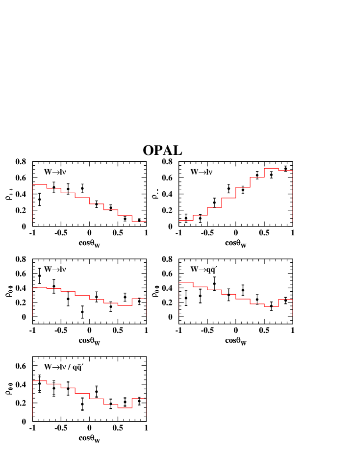
Figure 1: Luminosity-weighted averages of the diagonal elements of the SDM as functions of $\cos{\theta_{\mathrm{W}}}$. The points show the data after detector and bias corrections. The inner error bars show the statistical uncertainties and the outer error bars show the total uncertainties including both the statistical and systematic contributions. The histograms show the generator-level KandY MC prediction. The figures in the top row show $\rho_{++}$ and $\rho_{--}$ for leptonically decaying $\mathrm{W}$ bosons. The figures in the middle row show $\rho_{00}$ for leptonically decaying $\mathrm{W}$ bosons and hadronically decaying $\mathrm{W}$ bosons separately. The figure in the bottom row shows $\rho_{00}$ with the leptonic and hadronic decay modes combined. By construction, the diagonal elements of the SDM are related to each other by the normalisation condition $\rho_{++}+\rho_{--}+\rho_{00}=1$, but have not been individually constrained to the physically-allowed region between zero and one.

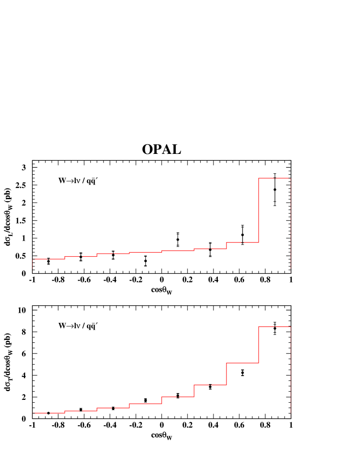
Figure 2: The luminosity-weighted average polarised differential cross-sections of section 2.3, where the average is over the eight nominal centre-of-mass energies and over the $\cos{\theta_{\mathrm{W}}}$ bin width. The points show the data after detector and bias corrections. The inner error bars show the statistical uncertainties and the outer error bars show the total uncertainties including both the statistical and systematic contributions. The histograms show the generator-level KandY MC prediction.

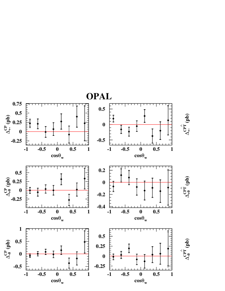
Figure 3: The luminosity-weighted average of the $\mathrm{CP}$-odd and $\mathrm{CP\hat{T}}$-odd observables of section 2.4, where the average is over the eight nominal centre-of-mass energies and over the $\cos{\theta_{\mathrm{W}}}$ bin width. The observables are measured in units of picobarns and shown as functions of $\cos{\theta_{\mathrm{W}}}$. The points show the data after detector correction. The inner error bars show the statistical uncertainties and the outer error bars show the total uncertainties including both the statistical and systematic contributions. The solid lines show the SM tree-level prediction.

References

- [1] G. Gounaris, J. Layssac, G. Moultaka and F.M. Renard, Int. J. Mod. Phys. A8 (1993) 3285.
- [2] Physics at LEP2, edited by G. Altarelli, T. Sjöstrand and F. Zwirner, CERN 96-01 Vol. 2, 11.
- [3] Physics at LEP2, edited by G. Altarelli, T. Sjöstrand and F. Zwirner, CERN 96-01 Vol. 1, 525.
- [4] L3 Collaboration, P. Achard et al., Phys. Lett. B557 (2003) 147.
- [5] OPAL Collaboration, G. Abbiendi et al., Eur. Phys. J. C19 (2001) 229.
- [6] OPAL Collaboration, G. Abbiendi et al., Eur. Phys. J. C8 (1999) 191.
- [7] G. Gounaris, D. Schildknecht and F.M. Renard, Phys. Lett. B263 (1991) 291.
- [8] K. Hagiwara, R.D. Peccei, D. Zeppenfeld and K. Hikasa, Nucl. Phys. B282 (1987) 253.
- [9] D. Chang, W. Keung and I. Phillips, Phys. Rev. D48 (1993) 4045.
- [10] ALEPH Collaboration, A. Heister et al., Eur. Phys. J. C21 (2001) 423.
- [11] OPAL Collaboration, K. Ahmet et al., Nucl. Instr. Meth. A305 (1991) 275.
- [12] B.E. Anderson et al., IEEE Trans. Nucl. Sci. 41 (1994) 845.
-
[13]
S. Jadach et al., Phys. Rev. D61 (2000) 113010;
S. Jadach et al., Comput. Phys. Commun. 140 (2001) 432. - [14] S. Jadach et al., Comput. Phys. Commun. 140 (2001) 475.
-
[15]
M. Skrzypek et al., Comput. Phys. Commun. 94 (1996) 216;
M. Skrzypek et al., Phys. Lett. B372 (1996) 289;
S. Jadach et al., Comput. Phys. Commun. 119 (1999) 272. -
[16]
F.A. Berends, R. Pittau and R. Kleiss, Comput. Phys. Commun. 85 (1995) 437;
F.A. Berends and A.I. van Sighem, Nucl. Phys. B454 (1995) 467. - [17] T. Sjöstrand, Comput. Phys. Commun. 82 (1994) 74.
- [18] G. Marchesini et al., Comput. Phys. Commun. 67 (1992) 465.
- [19] L. Lönnblad, Comput. Phys. Commun. 71 (1992) 15.
-
[20]
S. Jadach, B.F.L. Ward and Z. Wa̧s, Phys. Lett. B449 (1999) 97;
S. Jadach, B.F.L. Ward and Z. Wa̧s, Comput. Phys. Commun. 130 (2000) 260. - [21] J. Allison et al., Nucl. Instr. Meth. A317 (1992) 47.
- [22] OPAL Collaboration, G. Abbiendi et al., Phys. Lett. B493 (2000) 249.
- [23] OPAL Collaboration, K. Ackerstaff et al., Eur. Phys. J. C1 (1998) 395.
- [24] OPAL Collaboration, G. Abbiendi et al., Eur. Phys. J. C19 (2001) 1.
- [25] A. Höcker and V. Kartvelishvili, Nucl. Instr. Meth. A372 (1995) 469.
- [26] G. D. Agostini, Nucl. Instr. Meth. A362 (1995) 487.
- [27] OPAL Collaboration, K. Ackerstaff et al., Z. Phys. C74 (1997) 413.
- [28] Particle Data Group, K. Hagiwara et al., Phys. Rev. D66 (2002) 281.
- [29] OPAL Collaboration, G. Abbiendi et al., Phys. Lett. B507 (2001) 29.
- [30] L. Lyons, D.Gibaut and P. Clifford, Nucl. Instr. Meth. A270 (1988) 110.
- [31] HEPDATA: The Durham RAL Databases, Durham Database Group, Durham University (UK), http://www-spires.dur.ac.uk/HEPDATA.