EUROPEAN ORGANIZATION FOR NUCLEAR RESEARCH

CERN-EP-2003-082

28 November 2003

Measurement of the partial widths of the Z into up- and down-type quarks

The OPAL Collaboration

Using the entire OPAL LEP1 on-peak Z hadronic decay sample, $\rm Z\rightarrow q\bar{q}\gamma$ decays were selected by tagging hadronic final states with isolated photon candidates in the electromagnetic calorimeter. Combining the measured rates of $\rm Z\rightarrow q\bar{q}\gamma$ decays with the total rate of hadronic Z decays permits the simultaneous determination of the widths of the Z into up- and down-type quarks. The values obtained, with total errors, were

$$\Gamma_{\rm u}=300^{+19}_{-18}\quad{\rm MeV}\qquad{\rm and}\qquad\Gamma_{\rm d}=381^{+12}_{-12}\quad{\rm MeV}.$$

The results are in good agreement with the Standard Model expectation.

To be submitted to Physics Letters

The OPAL Collaboration

G. Abbiendi², C. Ainsley⁵, P.F. Åkesson^3,y, G. Alexander²², J. Allison¹⁶, P. Amaral⁹, G. Anagnostou¹, K.J. Anderson⁹, S. Arcelli², S. Asai²³, D. Axen²⁷, G. Azuelos^18,a, I. Bailey²⁶, E. Barberio^8,p, T. Barillari³², R.J. Barlow¹⁶, R.J. Batley⁵, P. Bechtle²⁵, T. Behnke²⁵, K.W. Bell²⁰, P.J. Bell¹, G. Bella²², A. Bellerive⁶, G. Benelli⁴, S. Bethke³², O. Biebel³¹, O. Boeriu¹⁰, P. Bock¹¹, M. Boutemeur³¹, S. Braibant⁸, L. Brigliadori², R.M. Brown²⁰, K. Buesser²⁵, H.J. Burckhart⁸, S. Campana⁴, R.K. Carnegie⁶, A.A. Carter¹³, J.R. Carter⁵, C.Y. Chang¹⁷, D.G. Charlton¹, C. Ciocca², A. Csilling²⁹, M. Cuffiani², S. Dado²¹, A. De Roeck⁸, E.A. De Wolf^8,s, K. Desch²⁵, B. Dienes³⁰, M. Donkers⁶, M. Doucet^b1, J. Dubbert³¹, E. Duchovni²⁴, G. Duckeck³¹, I.P. Duerdoth¹⁶, E. Etzion²², F. Fabbri², L. Feld¹⁰, P. Ferrari⁸, F. Fiedler³¹, I. Fleck¹⁰, M. Ford⁵, A. Frey⁸, P. Gagnon¹², J.W. Gary⁴, G. Gaycken²⁵, C. Geich-Gimbel³, G. Giacomelli², P. Giacomelli², M. Giunta⁴, J. Goldberg²¹, E. Gross²⁴, J. Grunhaus²², M. Gruwé⁸, P.O. Günther³, A. Gupta⁹, C. Hajdu²⁹, M. Hamann²⁵, G.G. Hanson⁴, A. Harel²¹, M. Hauschild⁸, C.M. Hawkes¹, R. Hawkings⁸, R.J. Hemingway⁶, G. Herten¹⁰, R.D. Heuer²⁵, J.C. Hill⁵, K. Hoffman⁹, D. Horváth^29,c, P. Hüntemeyer^c1, P. Igo-Kemenes¹¹, K. Ishii²³, H. Jeremie¹⁸, P. Jovanovic¹, T.R. Junk^6,i, N. Kanaya²⁶, J. Kanzaki^23,u, D. Karlen²⁶, K. Kawagoe²³, T. Kawamoto²³, R.K. Keeler²⁶, R.G. Kellogg¹⁷, B.W. Kennedy²⁰, K. Klein^11,t, A. Klier²⁴, S. Kluth³², T. Kobayashi²³, M. Kobel³, S. Komamiya²³, T. Krämer²⁵, P. Krieger^6,l, J. von Krogh¹¹, K. Kruger⁸, T. Kuhl²⁵, M. Kupper²⁴, G.D. Lafferty¹⁶, H. Landsman²¹, D. Lanske¹⁴, J.G. Layter⁴, D. Lellouch²⁴, J. Letts^o, L. Levinson²⁴, J. Lillich¹⁰, S.L. Lloyd¹³, F.K. Loebinger¹⁶, J. Lu^27,w, A. Ludwig³, J. Ludwig¹⁰, W. Mader³, S. Marcellini², A.J. Martin¹³, G. Masetti², T. Mashimo²³, P. Mättig^m, J. McKenna²⁷, R.A. McPherson²⁶, F. Meijers⁸, W. Menges²⁵, F.S. Merritt⁹, H. Mes^6,a, A. Michelini², S. Mihara²³, G. Mikenberg²⁴, D.J. Miller¹⁵, S. Moed²¹, W. Mohr¹⁰, T. Mori²³, A. Mutter¹⁰, K. Nagai¹³, I. Nakamura^23,v, H. Nanjo²³, H.A. Neal³³, R. Nisius³², S.W. O’Neale¹, A. Oh⁸, A. Okpara¹¹, M.J. Oreglia⁹, S. Orito^23,∗, C. Pahl³², G. Pásztor^4,g, J.R. Pater¹⁶, J.E. Pilcher⁹, J. Pinfold²⁸, D.E. Plane⁸, B. Poli², O. Pooth¹⁴, M. Przybycień^8,n, A. Quadt³, K. Rabbertz^8,r, C. Rembser⁸, P. Renkel²⁴, J.M. Roney²⁶, S. Rosati^3,y, Y. Rozen²¹, K. Runge¹⁰, K. Sachs⁶, T. Saeki²³, E.K.G. Sarkisyan^8,j, A.D. Schaile³¹, O. Schaile³¹, P. Scharff-Hansen⁸, J. Schieck³², T. Schörner-Sadenius^8,a1, M. Schröder⁸, M. Schumacher³, W.G. Scott²⁰, R. Seuster^14,f, T.G. Shears^8,h, B.C. Shen⁴, P. Sherwood¹⁵, A. Skuja¹⁷, A.M. Smith⁸, R. Sobie²⁶, S. Söldner-Rembold¹⁵, F. Spano⁹, A. Stahl^3,x, D. Strom¹⁹, R. Ströhmer³¹, S. Tarem²¹, M. Tasevsky^8,z, R. Teuscher⁹, M.A. Thomson⁵, E. Torrence¹⁹, D. Toya²³, P. Tran⁴, I. Trigger⁸, Z. Trócsányi^30,e, E. Tsur²², M.F. Turner-Watson¹, I. Ueda²³, B. Ujvári^30,e, C.F. Vollmer³¹, P. Vannerem¹⁰, R. Vértesi^30,e, M. Verzocchi¹⁷, H. Voss^8,q, J. Vossebeld^8,h, D. Waller⁶, C.P. Ward⁵, D.R. Ward⁵, P.M. Watkins¹, A.T. Watson¹, N.K. Watson¹, P.S. Wells⁸, T. Wengler⁸, N. Wermes³, D. Wetterling¹¹ G.W. Wilson^16,k, J.A. Wilson¹, G. Wolf²⁴, T.R. Wyatt¹⁶, S. Yamashita²³, D. Zer-Zion⁴, L. Zivkovic²⁴

¹School of Physics and Astronomy, University of Birmingham, Birmingham B15 2TT, UK
²Dipartimento di Fisica dell’ Università di Bologna and INFN, I-40126 Bologna, Italy
³Physikalisches Institut, Universität Bonn, D-53115 Bonn, Germany
⁴Department of Physics, University of California, Riverside CA 92521, USA
⁵Cavendish Laboratory, Cambridge CB3 0HE, UK
⁶Ottawa-Carleton Institute for Physics, Department of Physics, Carleton University, Ottawa, Ontario K1S 5B6, Canada
⁸CERN, European Organisation for Nuclear Research, CH-1211 Geneva 23, Switzerland
⁹Enrico Fermi Institute and Department of Physics, University of Chicago, Chicago IL 60637, USA
¹⁰Fakultät für Physik, Albert-Ludwigs-Universität Freiburg, D-79104 Freiburg, Germany
¹¹Physikalisches Institut, Universität Heidelberg, D-69120 Heidelberg, Germany
¹²Indiana University, Department of Physics, Bloomington IN 47405, USA
¹³Queen Mary and Westfield College, University of London, London E1 4NS, UK
¹⁴Technische Hochschule Aachen, III Physikalisches Institut, Sommerfeldstrasse 26-28, D-52056 Aachen, Germany
¹⁵University College London, London WC1E 6BT, UK
¹⁶Department of Physics, Schuster Laboratory, The University, Manchester M13 9PL, UK
¹⁷Department of Physics, University of Maryland, College Park, MD 20742, USA
¹⁸Laboratoire de Physique Nucléaire, Université de Montréal, Montréal, Québec H3C 3J7, Canada
¹⁹University of Oregon, Department of Physics, Eugene OR 97403, USA
²⁰CCLRC Rutherford Appleton Laboratory, Chilton, Didcot, Oxfordshire OX11 0QX, UK
²¹Department of Physics, Technion-Israel Institute of Technology, Haifa 32000, Israel
²²Department of Physics and Astronomy, Tel Aviv University, Tel Aviv 69978, Israel
²³International Centre for Elementary Particle Physics and Department of Physics, University of Tokyo, Tokyo 113-0033, and Kobe University, Kobe 657-8501, Japan
²⁴Particle Physics Department, Weizmann Institute of Science, Rehovot 76100, Israel
²⁵Universität Hamburg/DESY, Institut für Experimentalphysik, Notkestrasse 85, D-22607 Hamburg, Germany
²⁶University of Victoria, Department of Physics, P O Box 3055, Victoria BC V8W 3P6, Canada
²⁷University of British Columbia, Department of Physics, Vancouver BC V6T 1Z1, Canada
²⁸University of Alberta, Department of Physics, Edmonton AB T6G 2J1, Canada
²⁹Research Institute for Particle and Nuclear Physics, H-1525 Budapest, P O Box 49, Hungary
³⁰Institute of Nuclear Research, H-4001 Debrecen, P O Box 51, Hungary
³¹Ludwig-Maximilians-Universität München, Sektion Physik, Am Coulombwall 1, D-85748 Garching, Germany
³²Max-Planck-Institute für Physik, Föhringer Ring 6, D-80805 München, Germany
³³Yale University, Department of Physics, New Haven, CT 06520, USA

^a and at TRIUMF, Vancouver, Canada V6T 2A3
^c and Institute of Nuclear Research, Debrecen, Hungary
^e and Department of Experimental Physics, University of Debrecen, Hungary
^f and MPI München
^g and Research Institute for Particle and Nuclear Physics, Budapest, Hungary
^h now at University of Liverpool, Dept of Physics, Liverpool L69 3BX, U.K.
ⁱ now at Dept. Physics, University of Illinois at Urbana-Champaign, U.S.A.
^j and Manchester University
^k now at University of Kansas, Dept of Physics and Astronomy, Lawrence, KS 66045, U.S.A.
^l now at University of Toronto, Dept of Physics, Toronto, Canada
^m current address Bergische Universität, Wuppertal, Germany
ⁿ now at University of Mining and Metallurgy, Cracow, Poland
^o now at University of California, San Diego, U.S.A.
^p now at Physics Dept Southern Methodist University, Dallas, TX 75275, U.S.A.
^q now at IPHE Université de Lausanne, CH-1015 Lausanne, Switzerland
^r now at IEKP Universität Karlsruhe, Germany
^s now at Universitaire Instelling Antwerpen, Physics Department, B-2610 Antwerpen, Belgium
^t now at RWTH Aachen, Germany
^u and High Energy Accelerator Research Organisation (KEK), Tsukuba, Ibaraki, Japan
^v now at University of Pennsylvania, Philadelphia, Pennsylvania, USA
^w now at TRIUMF, Vancouver, Canada
^x now at DESY Zeuthen
^y now at CERN
^z now with University of Antwerp
^a1 now at DESY
^b1 now at NIST Center for Neutron Research and University of Maryland, Gaithersburg, MD, USA.
^c1 now at University of Utah, Department of Physics, Salt Lake City, UT 84112-0830, USA
^∗ Deceased

1 Introduction

Isolated hard photon production in hadronic Z decays provides information about the electroweak couplings of quarks and about QCD [1]. In $\mathrm{e^{+}e^{-}}$ collisions at the Z resonance, initial state radiation is suppressed and the production of isolated photons is mainly due to final state radiation (FSR) from the primary quark-antiquark pair.

The aim of the analysis of hadronic events with FSR presented in this paper is to measure the electroweak couplings to up- and down-type quarks. The measurement is based on the photon’s property of coupling to the electric charge. By selecting hadronic Z decays with FSR a subsample can be extracted which is enriched in up-type quarks since the strength of the coupling is proportional to the charge squared. Combining the measured rates of hadronic events with final state photon radiation with the total rate of hadronic Z decays permits the simultaneous determination of the partial decay widths into up-type and down-type quarks. This approach is complementary to analyses of partial decay widths dealing with either heavy or light quark flavour tagging. This analysis determines the electroweak coupling of the up-type quarks u, c and the down-type quarks d, s, b for the flavour admixture present on the Z resonance. The LEP experiments have already published QCD measurements and electroweak quark coupling measurements based on final state photon production [2, 3, 4, 5, 6, 7, 8, 9, 10]. This analysis is based on a larger data sample and updates earlier OPAL measurements [8].

The Z decay into a quark-antiquark pair can be described by effective vector and axial-vector couplings, $\bar{g}_{\rm V,q}$ and $\bar{g}_{\rm A,q}$, where q=u or d, representing up-type or down-type quarks. The Z decay widths depend on the sums of the squares of these couplings. Writing effective couplings $c_{\mathrm{q}}$ as

$$c_{\rm q}=4\left(\bar{g}^{2}_{\rm V,q}+\bar{g}^{2}_{\rm A,q}\right),$$ (1)

the total hadronic width of the Z, which is calculated to third order in $\alpha_{\mathrm{s}}$  [11], is given by:

$$\Gamma_{\rm hadrons}=\frac{N_{\mathrm{c}}m^{3}_{\rm Z}G_{\mathrm{F}}}{24\pi\sqrt{2}}\left(1+\frac{\alpha_{\mathrm{s}}}{\pi}+1.4\frac{\alpha_{\mathrm{s}}^{2}}{\pi^{2}}-12.8\frac{\alpha_{\mathrm{s}}^{3}}{\pi^{3}}\right)(2c_{\rm u}+3c_{\rm d}),$$ (2)

where $\alpha_{\mathrm{s}}$ is the strong coupling constant, $G_{\mathrm{F}}$ is the Fermi constant, $m_{\rm Z}$ is the mass of the Z, and $N_{\mathrm{c}}=3$ is the number of colours. The electromagnetic quark couplings also enter the hadronic partial width of the Z with a final state radiation (FSR) photon;

$$\Gamma_{{\rm hadrons}+\gamma}=\frac{N_{\mathrm{c}}m^{3}_{\rm Z}G_{\mathrm{F}}}{24\pi\sqrt{2}}F(y_{\rm cut})\frac{\alpha}{2\pi}(2q_{\rm u}^{2}c_{\rm u}+3q_{\rm d}^{2}c_{\rm d}),$$ (3)

where $\alpha$ is the electroweak coupling constant, $q_{\rm u}$ and $q_{\rm d}$ are the charges of up-type and down-type quarks, $F(y_{\rm cut})$ is a correction factor determined from perturbative calculations, and $y_{\rm cut}$ is a jet resolution parameter, which determines whether a photon is merged into a nearby jet. These widths can be re-written in terms of decay widths of the up- and down-type quarks:

$$\Gamma_{\rm hadrons}=2\Gamma_{\rm u}+3\Gamma_{\rm d};~{}\Gamma_{{\rm hadrons}+\gamma}=\frac{\alpha}{18\pi}\frac{F(y_{\rm cut})}{(1+\alpha_{\mathrm{s}}/\pi+1.4\alpha_{\mathrm{s}}^{2}/\pi^{2}-12.8\alpha_{\mathrm{s}}^{3}/\pi^{3})}(8\Gamma_{\rm u}+3\Gamma_{\rm d}).$$ (4)

The measurement of the partial hadronic width of the Z with an isolated FSR photon and the measurement of the total hadronic width of the Z depend on different linear combinations of $c_{\rm u}$ and $c_{\rm d}$, or equivalently of $\Gamma_{\rm u}$ and $\Gamma_{\rm d}$. In order to extract the partial widths or the couplings $c_{\rm u,d}$, the factor $F(y_{\rm cut})$ in equation 3 has to be calculated. Matrix element calculations at $\cal{O}(\alpha\alpha_{\rm s})$ are available to perform these calculations as a function of the jet resolution parameter $y_{\rm cut}$ [12]. One important aspect of these predictions is the regions of phase space in which they are valid. In particular, infrared divergences due to soft photons and photons collinear with soft quarks must be avoided. For this reason, hard isolated photons are studied. A good agreement between hard isolated photon production and matrix element predictions has already been demonstrated by OPAL [13]. In the range of intermediate values of $y_{\rm cut}$, $F(y_{\rm cut})$ can be determined with a theoretical uncertainty of around 1% based on these predictions. The uncertainty is evaluated by varying $\alpha_{\rm s}$ and the phase space cut-off in the perturbative calculation as described in more detail in section 6. In contrast to the procedure followed in reference [9] no correction to account for the b-quark mass is included in the equations (2) and (3). The results of the present analysis were extracted at effective masses of the photon-jet system where the relative impact of the b-quark mass is much smaller than in the case of reference [9].

In this paper, we present a new measurement of the partial widths $\Gamma_{\rm u}$ and $\Gamma_{\rm d}$. The full LEP1 data sample taken at the peak of the Z resonance was used in this analysis, amounting to more than 3 million hadronic Z decays. After describing the main characteristics of the OPAL detector in section 2, a description of the event selection follows in section 3. The background and efficiency corrections applied to the selected data are described in section 4. The systematic errors are discussed in section 5 before the results are presented in section 6.

2 The OPAL Detector

The OPAL detector operated at the LEP $\mbox{e}^{+}\mbox{e}^{-}$ collider at CERN. A detailed description of the detector can be found in reference [14]. For this study, the most important components of OPAL were the central detector and the barrel electromagnetic calorimeter. The central detector, measuring the momentum of charged particles, consisted of a system of cylindrical tracking chambers surrounded by a solenoidal coil which produced a uniform axial magnetic field of 0.435 T along the beam axis .

The electromagnetic calorimeters completely covered the azimuthal range for polar angles satisfying $|\cos\theta|<0.98$, providing excellent hermeticity. The barrel electromagnetic calorimeter covered the polar angle range $|\cos\theta|<0.82$. It consisted of 9440 lead glass blocks, each 24.6 radiation length deep, approximately pointing towards the interaction region. Each block subtended an angular region of approximately $40\times 40~{}\rm{mrad}^{2}$. Half of the block width corresponded to 1.9 Molière radii. Deposits of energy in adjacent blocks were grouped together to form clusters of electromagnetic energy. The intrinsic energy resolution of $\rm{\sigma_{E}/E=0.2\%\oplus 6.3\%/\sqrt{E}}$ was substantially degraded (by a factor $\simeq 2$) by the presence of two radiation lengths of material in front of the lead glass. For the intermediate region, $0.72<|\cos\theta|<0.82$, the amount of material increased to up to eight radiation lengths. The two endcap calorimeters, each made of 1132 lead glass blocks, 22 radiation lengths deep, covered the region of $0.81<|\cos\theta|<0.98$. In this study the measurement of inclusive photon production is restricted to the barrel part of the detector.

3 Event selection and reconstruction

The first stage of the event selection was to identify hadronic Z decays. In this sample, isolated, high energy, neutral clusters in the electromagnetic calorimeter were then considered as photon candidates. To reduce the dominant background from $\pi^{0}$ decays, the shower shapes were additionally required to be consistent with a shower produced by a single photon, as opposed, for example, to overlapping showers from the two photons from a $\pi^{0}$ decay. Jets were then reconstructed in events with a photon candidate. The jet reconstruction implied an additional isolation requirement on the photons, as a function of the jet resolution parameter.

Hadronic Z decays were selected from the data taken by the OPAL detector between 1990 and 1995 at a centre-of-mass energy of 91.2 GeV. The data taken above and below the Z resonance during those years were not analysed. Using the criteria described in reference [15], $N_{\mathrm{{Z}\rightarrow Hadrons}}=$ 3 022 897 hadronic Z decay candidates were selected. The tracks and clusters were defined as described in reference [16].

Isolated electromagnetic clusters in the electromagnetic calorimeter were identified within the selected sample. The following criteria were used:

1. Only clusters with no associated tracks were considered.

2. The clusters had to be located in the barrel region of the electromagnetic calorimeter defined by $|\cos\theta_{\rm cluster}|\leq 0.72$. This requirement reduces the background from initial state radiation, which peaks at low polar angle.

3. The energy of each cluster was required to be larger than 7 GeV. This reduces the background from neutral hadron decays and initial state radiation. It also enabled the use of a shower shape fit, for which the description of the Monte Carlo was not satisfactory below 7 GeV.

4. The shape of the cluster was required to be consistent with a single photon. The number $N_{\rm blocks}$ of lead glass blocks contributing more than 0.02 GeV to the cluster energy was required to be less than 16. A cut at $W<30$ mrad was set on the energy weighted first moment of the cluster, defined as:
   

   $$W=\sqrt{\frac{\sum_{i=1}^{N_{\rm blocks}}E_{i}^{\rm meas}\left((\phi_{i}-\bar{\phi})^{2}+(\theta_{i}-\bar{\theta})^{2}\right)}{\sum_{i=1}^{N_{\rm blocks}}E_{i}^{\rm meas}}},$$ (5)

   where $E_{i}^{\rm meas}$, $\phi_{i}$ and $\theta_{i}$ are the energy deposited in block $i$, its azimuthal and polar angles. $\bar{\phi}$ and $\bar{\theta}$ are the $\phi$ and $\theta$ positions of the cluster centroid. In addition, the shower-shape parameter $C$ was required to be smaller than 5. The same definition of $C$ as in [17] was used:

   $$C=\frac{1}{N_{\rm blocks}}\sum_{i}\frac{(E_{i}^{\rm pred}-E_{i}^{\rm meas})^{2}}{(\sigma_{i}^{\rm pred})^{2}+(\sigma_{i}^{\rm meas})^{2}},$$ (6)

   where $E_{i}^{\rm pred}$ is the predicted energy in calorimeter block number $i$. This was taken from the best fit of the shower profile parametrisation to the observed energy sharing between the calorimeter blocks assuming that the cluster was produced by an isolated photon. The reference profiles varied as a function of $\cos\theta$ because of the varying amount of material in front of the calorimeter. $\sigma_{i}^{\rm pred}=0.05\cdot E_{i}^{\rm pred}$ is the error on $E_{i}^{\rm pred}$ where 0.05 is the accuracy of the Monte Carlo integration and $\sigma_{i}^{\rm meas}=0.002\cdot E_{i}^{\rm meas}\oplus 0.063\sqrt{E_{i}^{\rm meas}}$ is the estimated error on $E_{i}^{\rm meas}$ [14].

5. The cluster candidates were required to be isolated. Clusters with tracks or other clusters of an energy sum greater than 0.5 GeV within a cone of half opening angle of 0.235 rad around the cluster were rejected.

In total, 12 626 events with a photon candidate were selected from the original sample of hadronic Z decays. Each event in the sample was reconstructed into jets. Two jet finding schemes were used and compared: Jade E0 [18] and Durham [19]. Both are based on the resolution parameter

$$y_{ij}=\frac{M^{2}_{ij}}{E^{2}_{\mathrm{v}is}}$$ (7)

where $E_{\mathrm{v}is}$ is the total visible energy in the detector. In the Jade algorithm $M_{ij}$ is defined as the invariant mass

$$M_{ij}^{2~{}\mathrm{{\sc Jade}}}=2E_{i}E_{j}(1-\cos\alpha_{ij}),$$ (8)

while in the Durham or $k_{T}$ algorithm it is defined as the minimum transverse momentum of one particle with respect to the other,

$$M_{ij}^{2~{}\mathrm{Durham}} = 2{\mathrm{m}in}(E_{i}^{2},E_{j}^{2})(1-\cos\alpha_{ij}),$$ (9)

where $E_{i}$, $E_{j}$ are the energies of the particles and $\alpha_{ij}$ is the angle between them. In each case, the jet finding was performed in two steps. In the first step, the jets were reconstructed excluding the photon candidate by iteratively combining particles until for all possible particle combinations the calculated $y_{ij}$ was larger than a specified $y_{\rm cut}$. This was done for 12 values of $y_{\rm cut}$ in both algorithms. In the second step, $y_{\gamma i}$ was calculated for the photon candidate and each jet $i$ in the event. Each value of $y_{\gamma i}$ was required to be greater than the $y_{\rm cut}$ used during the first step. Events failing this requirement were rejected. The number of events $n_{\rm raw}$ passing this last selection criterion depends on the chosen $y_{\rm cut}$ value. The choice of values for the $y_{\rm cut}$ in each algorithm ensured that the photon candidate was sufficiently isolated from the jets and provided a scan of the phase space to allow a valid and more detailed comparison of the result with matrix element calculations. The selected sample size for different $y_{\rm cut}$ values is shown in table 1 for the two jet finding schemes.

4 Background and efficiency corrections

The number of selected events was corrected for background contributions, detector response and selection efficiency. Two categories of background were considered. The first was the contribution from misidentified neutral hadrons and their decay products. The second was from genuine photons originating from initial state radiation. The sequence in which the data were corrected for background and efficiency reflects this difference in background sources. First, the background contribution from neutral hadrons was estimated by a fit to the shower shape distribution in data, using the difference in shower shape to distinguish genuine photons from hadron background. Second, a correction for detector effects was applied. In particular this corrected for the photon detection efficiency and compensated for the requirements on the shower shape and measurement uncertainties. It was calculated using a full simulation of the OPAL detector. Third, events with photons produced by ISR were subtracted. Their number was estimated with Monte Carlo simulations at the hadron level. Finally, the number of events remaining at the hadron level was corrected for hadronisation and selection efficiencies, so that it could be compared with results from matrix element calculations at the parton level. In this analysis, hadron and parton level were defined as in reference [20].

4.1 Neutral hadrons

Neutral hadrons and their decay products can produce isolated clusters in the electromagnetic calorimeter which pass the selection for photon candidates. This background was simulated using a sample of 8.4 million events generated with Jetset 7.4 [21], which were processed with the OPAL detector simulation program [22]. The hadronic background comes mainly from events with a $\pi^{0}$ decay, and has a small contribution from $\eta$ decays and K${}^{0}_{L}$. There is also a contribution below 1% of the total hadronic background from neutrons, $\omega$ and $\rho$. The simulated $C$ distributions are shown in figure LABEL:fig-c_dist_mc for single photon clusters and for clusters produced by the hadronic background sources. By fitting the data distribution to a linear combination of the expected distribution of the shower-shape parameter $C$ for the background and the measured distribution for single photons taken from a data sample of $\mu\mu\gamma$ events, the fraction of single photon events was extracted [3]. In figure LABEL:fig-c_dist_mu the $C$ distributions are plotted for isolated neutral clusters from $\mu\mu\gamma$ events in data and Monte Carlo and good agreement is observed. The fit is a binned maximum likelihood fit which takes into account the effects of data and Monte Carlo statistics [23]. For each $y_{\rm cut}$ value considered, the fit was performed in eight cluster energy bins to extract the fraction of single photon events. The total fraction $f_{\gamma}({y_{\rm cut}})$ of single photon events for each $y_{\rm cut}$ value was estimated by calculating the weighted average of the results for the eight energy bins. The procedure was repeated for the two jet finding algorithms. Figure 3 shows an example of the fit results for the eight cluster energy bins. The jet finding scheme was in this case Jade E0, with $y_{\rm cut}=0.08$. Table 2 shows the extracted fraction of single photon events in the selected samples for three of the $y_{\rm cut}$ values in each jet finding scheme, spanning the phase space studied. The quoted $68.3\%$ confidence level error was obtained by studying the variation of $\ln{\mathcal{L}}$ [23]. It combines the uncertainty due to limited data statistics (2526 $\mu\mu\gamma$ events, and between 1900 and 9000 candidates, see table 1) and due to limited Monte Carlo statistics (between 548 and 1695 clusters from neutral hadrons).

The background estimate was found to be consistent with previous measurements performed by OPAL and L3. OPAL measured [24] that Jetset underestimates the rate of isolated $\eta$ with an energy $E_{\eta}>4.5$ GeV by a factor $2.07\pm 0.11$, and the rate of isolated $\pi^{0}$ in the energy range $4.5<E_{\pi^{0}}<22.8$ GeV by a factor $1.99\pm 0.05$. L3 measured [25] a rate of isolated electromagnetic clusters which was $1.88\pm 0.08$ times larger than predicted by Jetset. Applying the present method to our data sample over a range of cluster energies $4.5<E_{\rm clust}<46$ GeV, we measured an excess of a factor $2.05\pm 0.03$. The value is compatible with the previous measurements of OPAL and L3.

4.2 Detector Effects

After subtracting the events with an isolated neutral hadron from the sample of candidates, the data were corrected for detector effects:

$$n_{\rm had}^{\gamma}({y_{\rm cut}})=n_{\rm raw}({y_{\rm cut}})\times f_{\gamma}({y_{\rm cut}})\times c^{\rm det}({y_{\rm cut}})$$ (10)

with $n_{\rm raw}({y_{\rm cut}})$ as the number of photon events before the background correction, and $f_{\gamma}({y_{\rm cut}})$ as the fitted single photon fraction (ISR+FSR) in the selected sample at detector level, which has been derived as discussed in the previous section. The correction factor $c^{\rm det}({y_{\rm cut}})$, which takes into account detector inefficiencies, was calculated for each $y_{\rm cut}$ and each jet finding algorithm using the sample of 8.4 million fully simulated Jetset events. The same cuts on the photon energy, polar angle and isolation were applied at the hadron level. The correction factors $c^{\rm det}({y_{\rm cut}})$ are shown in table 2, again for three values of $y_{\rm cut}$ in each jet finding scheme. The efficiency losses are mainly due to photon conversions in the two radiation lengths of material in front of the electromagnetic calorimeter, e.g. the beam pipe, the central tracking system and the magnet coil. The photon conversion rate was calculated to be around 8%.

4.3 Initial state radiation

Initial state radiation photons are indistinguishable from photons from final state radiation. Although the energy and angular cuts on the electromagnetic clusters reduce the amount of initial state radiation, which is already small when working at the Z resonance, initial state photons can still make a contribution of several percent to the selected sample. This contribution was evaluated using the $\cal{KK}$ Monte Carlo [26] without the full detector simulation; the $\cal{KK}$ generator has the most accurate ISR modeling for $\mathrm{e^{+}e^{-}}$collisions. The data which are corrected for detector effects are directly comparable to the $\cal{KK}$ hadron level predictions. The number of FSR events at the hadron level is therefore given by

$$n^{\rm FSR}_{\rm had}({y_{\rm cut}})=n_{\rm had}^{\gamma}({y_{\rm cut}})-b^{\rm ISR}({y_{\rm cut}}),$$ (11)

with $b^{\rm ISR}({y_{\rm cut}})$ as the number of ISR events as calculated with the $\cal{KK}$ Monte Carlo program and normalized to the number $N_{\mathrm{{Z}\rightarrow Hadrons}}$ of selected hadronic Z decays. The same cuts on the photon energy, polar angle and isolation were applied at the hadron level for both the Jetset and $\cal{KK}$ Monte Carlo samples. The numbers of isolated initial state photons $b^{\rm ISR}({y_{\rm cut}})$ to be subtracted are shown in table 2 for three values of $y_{\rm cut}$ in each jet finding scheme.

4.4 Geometrical acceptance, isolation cone, and hadronisation

In order to compare the measured final state photon rate with the matrix element predictions, the measurements must be corrected for the remaining acceptance cuts on the polar angle and the cone isolation, for hadronisation, and for fragmentation, which affect the number of jets in the event. A correction factor $c^{\rm par}({y_{\rm cut}})$ which takes into account the cuts mentioned above was calculated using Jetset 7.4. No further correction was made for the energy cut $E_{\rm clust}>7$ GeV, to avoid introducing additional uncertainties. The matrix element predictions were calculated with the same requirement, $E_{\gamma}>7$ GeV. The correction factors $c^{\rm par}({y_{\rm cut}})$ for three different $y_{\rm cut}$ values in two jet finding algorithms are shown in table 2. The corrected numbers of isolated final state photon candidates per 1000 hadron events,

$$R_{\rm FSR}=n^{\rm FSR}_{\rm par}({y_{\rm cut}})\times\frac{1000}{N_{\mathrm{{Z}\rightarrow Hadrons}}}\\ =n^{\rm FSR}_{\rm had}({y_{\rm cut}})\times c^{\rm par}({y_{\rm cut}})\times\frac{1000}{N_{\mathrm{{Z}\rightarrow Hadrons}}},$$ (12)

are shown in table 1.

5 Systematic Effects

The contributions to the systematic uncertainty are summarized in table 3. Relative errors are given for the value of $y_{\rm cut}$ in each scheme which minimizes the total uncertainty on the photon rate, and for the extreme $y_{\rm cut}$ values considered. The statistical uncertainty quoted in table 3 combines the error from limited data and Monte Carlo statistics. It is calculated as the quadrature sum of the fit error (see section 4.1) and of the uncertainties of all Monte Carlo samples generated and used to simulate various other aspects of the analysis. The systematic studies from which the other uncertainties were obtained are described below.

5.1 Background

The estimate of the hadronic background which results from the fit of the shower-shape parameter $C$ relies on the proper simulation of the shower for the background, as well as on the simulation of the yield of the various hadronic background sources. To quantify the systematic uncertainty originating from the description of the hadronic background, the fit procedure was repeated for all $y_{\rm cut}$ values and the two jet finding algorithms after changing the Monte Carlo input distributions to which the data are fitted by varying the composition of the hadronic background. The contribution from $\pi^{0}$ and $\eta$ was doubled to account for the observed underestimation of isolated neutral pions and $\eta$-mesons in the Monte Carlo [24]. The contribution from K${}^{0}_{L}$ was increased by 18%, which was extrapolated from the observed differential cross-section in [27]. The observed differences from the results of the default procedure were not statistically significant, and showed no systematic trend, so no systematic uncertainty was assigned. Further systematic studies have been made by varying the bin size and the upper boundary of the $C$ distribution. Again, no significant change in the resulting rate was observed.

The effect of the interference between initial state radiation and final state radiation was checked by comparing prompt photon samples from the $\cal{KK}$ Monte Carlo generated with and without ISR-FSR interference. The average difference of around 1 per mill in the rate of isolated prompt photons with an energy of larger than 7 GeV was assigned as systematic uncertainty on the corrected rate and is listed in table 3.

5.2 Detector description

Several systematic effects coming from the description of the detector were investigated:

• The track parameters were smeared by 10% to estimate the effect of the reconstruction on the jet finding and the isolation criteria [28].

• The effect of the energy resolution of the electromagnetic calorimeter was evaluated by smearing the energy of clusters by 20%. This number is chosen since the energy resolution of isolated photon clusters selected in Jetset and in a $\mu\mu\gamma$ reference data sample differ by up to 20%. The cluster energies were also shifted by 0.1-0.2 GeV. This shift reflects the difference in the mean values of the distributions of $E_{\rm cluster}-E_{\gamma}$ from the simulation and of $E_{\rm cluster}-E_{\rm kin}$ in data, where $E_{\rm kin}$ is the kinematically reconstructed energy of the isolated photon in the reference sample.

These effects would modify the correction factor $c^{\rm det}({y_{\rm cut}})$. In all cases, the systematic uncertainty on the correction factor was found to be below the per mill level.

An important contribution to the systematic error comes from the simulation of photon conversions. An error of 10% on the photon conversion rate [29] results in an error on the correction factor of about 0.8%.

The jet reconstruction was also tested for systematic effects. The energy resolution was checked using a subsample of the candidate events with two jets and one isolated photon. The measured energy of each jet was compared to the energy of the same jet calculated by imposing energy/momentum conservation in the final state. The measured shift in the jet energy was used to estimate the systematic error on the photon rate. A variation between 0.1% and 0.6% in the rate of photons was found for the Jade E0 jet finding scheme as a function of $y_{\rm cut}$, and between 0.1% and 0.3% for the Durham scheme.

The jet angle reconstruction was tested using the same sample of two-jet events. The hadronic part of each event in both Monte Carlo and data was boosted into its centre of mass using the photon momentum. In this system the two jets should be collinear. The angular shift between the Monte Carlo expectation and the data was taken to calculate a systematic uncertainty. This uncertainty varied between 0.1% and 1.7% for both jet finders. Studies of the photon angular resolution showed that the effect on the rate was negligible.

The combined systematic uncertainties obtained from these studies are given in table 3 as the contribution to the error from the determination of the correction factor $c^{\rm det}({y_{\rm cut}})$.

5.3 Fragmentation and hadronisation

Three methods were used to evaluate the uncertainty arising from fragmentation and hadronisation. They affect the determination of the correction factor $c^{\rm par}({y_{\rm cut}})$, which compensates for the geometrical acceptance, i.e. the extrapolation of the result to the total $\cos\theta$ range, and for the isolation cone around the photon candidate. An uncertainty is not trivial to assign since we largely rely on Monte Carlo studies.

• Parton shower model
  The Jetset predictions were compared with those of Herwig[30] and Ariadne [31], which use different parton showering schemes. Herwig also uses a different fragmentation scheme. The relative deviations are larger towards the ends of the $y_{\rm cut}$ range with a largest deviation of $-9.0\%$ (for Herwig and the Durham algorithm). The deviations are smaller in the intermediate range of $y_{\rm cut}$ values for both jet finder schemes. The deviations stem from the different particle flow around the FSR photons in the three models. As a result, in the Jetset case more photons are rejected at the hadron level than in the Herwig or Ariadne cases due to the cone isolation requirement. This effect is smaller in the region of intermediate $y_{\rm cut}$ values.

• First derivative prediction
  The photon rates measured with different $y_{\rm cut}$ values are correlated. The first derivative of the photon rate is almost statistically independent for the different $y_{\rm cut}$ values. Comparing the first derivative distribution for different parton shower models provides an additional systematic cross-check of the efficiency correction. The first derivative is defined as

  $$D_{\rm FSR}(y_{\rm cut}) = \frac{1}{N_{\mathrm{{Z}\rightarrow Hadrons}}\delta}[N_{\rm FSR}(y_{\rm cut}-\delta/2)-N_{\rm FSR}(y_{\rm cut}+\delta/2)]$$ (13)

  $$= \frac{1}{N_{\mathrm{{Z}\rightarrow Hadrons}}\delta}[\sum_{i}N^{i\rightarrow{\rm reject}}-\sum_{i}N^{{\rm reject}\rightarrow i}],$$

  where $N_{\rm FSR}$ is the number of final state photon candidates. $N^{i\rightarrow{\rm reject}}$ is the number of events that have a jet multiplicity $i$ at ${y_{\rm cut}}-\delta/2$ but that are rejected at ${y_{\rm cut}}+\delta/2$, whereas $N^{{\rm reject}\rightarrow i}$ is the number of events that are rejected at ${y_{\rm cut}}-\delta/2$ but are retained at ${y_{\rm cut}}+\delta/2$ with a jet multiplicity $i$. The gains and losses for each $i$-jet event class are statistically independent, so that the quantities,

  $$c^{i\rightarrow{\rm reject}}=\frac{N_{\rm parton}^{i\rightarrow{\rm reject}}}{N_{\rm hadron}^{i\rightarrow{\rm reject}}}\qquad{\rm and}\qquad c^{{\rm reject}\rightarrow i}=\frac{N_{\rm parton}^{{\rm reject}\rightarrow i}}{N_{\rm hadron}^{{\rm reject}\rightarrow i}}$$ (14)

  are also almost statistically independent. The discrepancy between these quantities calculated for Herwig and Jetset is largest for small $y_{\rm cut}$ values. Relative to the Jetset value, it amounts to up to –18.5% for the Jade E0 scheme and up to –24.1% in the Durham scheme. For ${y_{\rm cut}}>0.02$, the predictions agree to within 6% for the Jade E0 scheme. For the Durham scheme, they agree within 10% for ${y_{\rm cut}}>0.008$. The deviations are also due to the cone isolation criterion.

• Isolation cone
  The analysis was repeated with different isolation cones, varying between 0.175 rad and 0.335 rad and allowing for up to 0.5 GeV of additional energy within the isolation cone. The largest deviations are observed for a cone of $0.175$ rad half angle. For the Jade E0 jet finder, they are below $5\%$ for all values of ${y_{\rm cut}}$ and have a peak value of $4.9\%$ for ${y_{\rm cut}}=0.2$. The deviations calculated in the Durham scheme are at the same level, with the highest value of $4.8\%$ at the largest ${y_{\rm cut}}=0.1$.

Because the previous considerations are not independent, the estimates which give the largest positive and the largest negative contributions to the systematic uncertainty for each $y_{\rm cut}$ have been assigned as systematic errors on the photon rate. They are listed in table 3 as the error contribution from the determination of $c^{\rm par}({y_{\rm cut}})$ and they are typically largest for small $y_{\rm cut}$ values, smaller for intermediate $y_{\rm cut}$ values, and increase again for large $y_{\rm cut}$ values. This indicates that the correction $c^{\rm par}({y_{\rm cut}})$ and therefore the final result is more sensitive to details of the energy flow around the photon candidate for very large and very small values of ${y_{\rm cut}}$, i.e. near the phase space boundaries.

6 Results

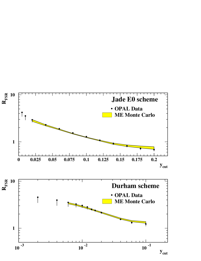
Figure 4: The total number of events with FSR per 1000 hadron events in two jet finder schemes and for twelve values of $y_{cut}$. The prediction of the ${\mathcal{O}}(\alpha\alpha_{\mathrm{s}}^{(1)})$ matrix element Monte Carlo is also shown. The band width of the theoretical prediction is a result of a variation of $\alpha_{\mathrm{s}}^{(1)}$ and of the phase space cut-off in the perturbative calculations.

Figure 4 shows the measured rate of FSR photons normalised to 1000 hadronic Z decays as a function of the $y_{\rm cut}$ value for the two jet finding algorithms. The results are compared to bands of matrix element Monte Carlo predictions for $0.15<\alpha^{(1)}_{\mathrm{s}}<0.22$ and $0.0005<y_{\gamma}<0.001$. $\alpha^{(1)}_{\mathrm{s}}$ is the first order $\alpha_{\mathrm{s}}$ value and $y_{\gamma}$ is the cut-off in the phase space of the photon emission which is used in the matrix element calculations to remove the singularity of the $y_{q\gamma}$,$y_{\bar{q}\gamma}$ poles [8, 12, 13, 4]. The lowest two values of $y_{\rm cut}$ in both jet finder schemes are not considered because of the large contribution from events with more than three jets, which are not described by the matrix element calculations. For both jet finding algorithms, the measurement errors in the intermediate $y_{\rm cut}$ range are smaller than in the regions of small and large $y_{\rm cut}$ values. At small and large $y_{\rm cut}$ values, the result is particularly sensitive to the isolation cone requirement, causing a large efficiency loss and a large systematic error.

The decay widths $\Gamma_{\rm u}$ and $\Gamma_{\rm d}$ can be calculated from the measured FSR photon rate. The value ${y_{\rm cut}}=0.08$ for the Jade E0 jet finding algorithm and ${y_{\rm cut}}=0.016$ for Durham were chosen for the final results since they are the values for which the error on the FSR photon rate is the smallest. Taking a value of $\alpha_{\mathrm{s}}^{(1)}=0.18\pm 0.03$ [32], correction factors $F(y_{\rm cut})$ of $9.60^{+0.16}_{-0.13}$ (${y_{\rm cut}}=0.016$, Durham scheme) and $6.11^{+0.01}_{-0.06}$ (${y_{\rm cut}}=0.08$, Jade E0 scheme) were calculated to be used as input to equation 3. With values of $\alpha_{s}=0.1172\pm 0.002$ and $\Gamma_{\rm hadrons}=1744.4\pm 2.0$ MeV [33] entering equation 2, we obtain

$$8\Gamma_{\rm u}+3\Gamma_{\rm d}=3.55\pm 0.08^{+0.07+0.03}_{-0.07-0.01}\;\;{\rm GeV}$$ (15)

for the Jade E0 jet finding algorithm (${y_{\rm cut}}=0.08$) and

$$8\Gamma_{\rm u}+3\Gamma_{\rm d}=3.50\pm 0.09^{+0.10+0.05}_{-0.14-0.06}\;\;{\rm GeV}$$ (16)

for Durham (${y_{\rm cut}}=0.016$). The first error is due to statistics, the second error is due to systematics and the third error comes from the uncertainty in $\alpha_{\mathrm{s}}^{(1)}$ and the theoretical cut off $y_{\gamma}$. The results derived with the Jade and Durham schemes are consistent and the result with the smaller uncertainty (Jade scheme) is considered the main result.

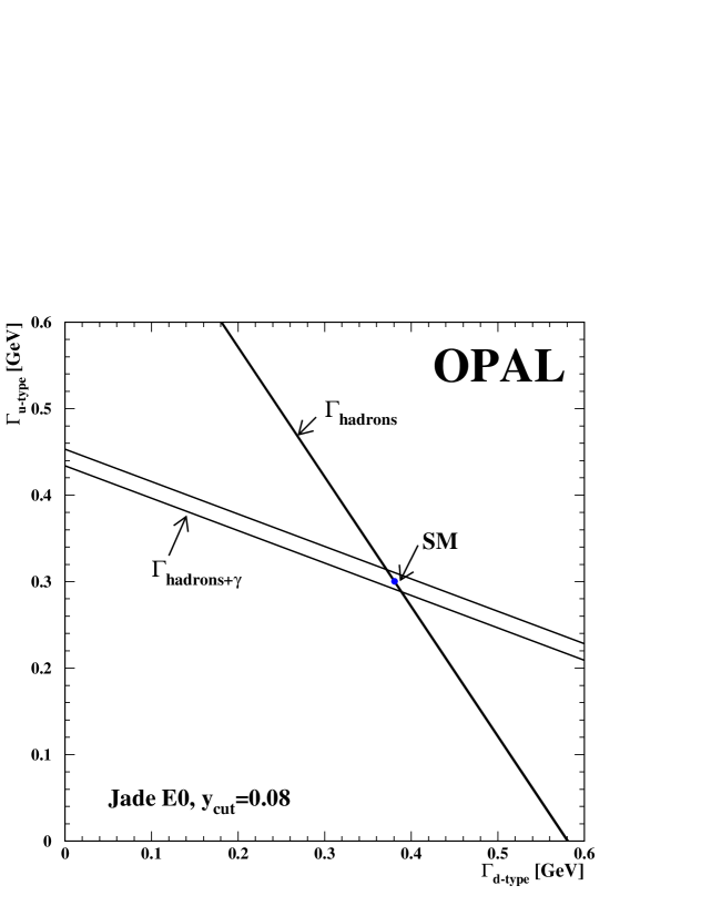
Figure 5: Correlation between the Z decay widths to up-type and down-type quarks. The band width of $\Gamma_{\rm hadrons+\gamma}=8\Gamma_{\rm u}+3\Gamma_{\rm d}$ reflects one standard deviation as obtained from this measurement. The narrow band shows the correlation within one standard deviation as obtained from the world average of $\Gamma_{\rm hadrons}=2\Gamma_{\rm u}+3\Gamma_{\rm d}$. The point on the narrow band represents the Standard Model expectation.

Figure 5 shows the correlation between the Z decay widths in up-type and down-type quarks obtained from this measurement. Also shown are the Standard Model prediction and the correlation obtained from the measurement of $\Gamma_{\rm hadrons}=2\Gamma_{\rm u}+3\Gamma_{\rm d}$. Combining the information on $\Gamma_{{\rm hadrons}+\gamma}$ and $\Gamma_{\rm hadrons}$, the decay widths for up-type and down-type quarks can be extracted for $y_{cut}=0.08$ in the Jade scheme:

$$\Gamma_{\rm u}=300\pm 13^{+12+5}_{-12-1}\quad{\rm MeV}\qquad{\rm and}\qquad\Gamma_{\rm d}=381\pm 9^{+8+1}_{-8-4}\quad{\rm MeV}.$$

Note that in this measurement $\Gamma_{\rm u}$ and $\Gamma_{\rm d}$ are 100% anti-correlated. The Standard Model predictions [33] for these widths are:

$$\Gamma_{\rm u}=300.3\pm 0.14\quad{\rm MeV}\qquad{\rm and}\qquad\Gamma_{\rm d}=380.7\pm 0.15\quad{\rm MeV}$$

in good agreement with the measurement. The result is also in good agreement with previous measurements from DELPHI [10], L3 [9], and OPAL [8, 34] and is significantly more precise. The analysis in [34] used high-momentum stable particles as a tag, while the other three were based on the determination of the FSR rate in hadronic Z decays.

7 Conclusion

Using the entire OPAL LEP1 on-peak Z hadronic decay sample a measurement of the partial decay widths of the Z into up- and down-type quarks was performed. The measurement was based on 12 626 observed candidate hadronic Z decays with final state photon emission. The partial width $\Gamma_{{\rm hadrons}+\gamma}$ for such decays was calculated as a function of the partial widths of the Z into up- and down-type quarks with the aid of a matrix element Monte Carlo program of $\cal{O}(\alpha\alpha_{\rm s})$. The calculated value for $\Gamma_{{\rm hadrons}+\gamma}$ was combined with the PDG average of the total hadronic Z width $\Gamma_{\rm hadrons}$ to determine $\Gamma_{\rm u}=300^{+19}_{-18}$ MeV and $\Gamma_{\rm d}=381^{+12}_{-12}$ MeV. The result is consistent with the Standard Model expectation and with previous measurements [8, 9, 10, 34]. Its precision is significantly improved compared to previous measurements using a similar method of selecting hadronic Z decays with highly isolated and energetic photons due to increased data and Monte Carlo statistics. With respect to the previous OPAL measurement [8] a different approach was chosen to estimate the background rate of neutral hadrons being misidentified as genuine photons. The previous measurement invokes isospin symmetry to estimate the background rate of neutral hadrons and measures the rate of isolated charged pions to extract the rate of isolated neutral pions. The present analysis utilises the different shapes of the distribution of the shower-shape parameter $C$ for neutral hadrons and genuine photons. The larger data and Monte Carlo statistics allowed us to choose this method which exhibits a smaller systematic uncertainty.

Jade E0			Durham ($k_{t}$)
$y_{cut}$	$n_{\rm raw}$	$R_{\rm FSR}$	$y_{cut}$	$n_{\rm raw}$	$R_{\rm FSR}$
0.005	8503	$4.22\pm 0.06$	0.002	8936	$4.55\pm 0.07$
0.01	7504	$3.55\pm 0.06$	0.004	8017	$3.96\pm 0.06$
0.02	6351	$2.93\pm 0.05$	0.006	7331	$3.53\pm 0.06$
0.04	5039	$2.31\pm 0.05$	0.008	6876	$3.25\pm 0.06$
0.06	4140	$1.89\pm 0.04$	0.01	6366	$3.04\pm 0.05$
0.08	3496	$1.54\pm 0.03$	0.012	5996	$2.83\pm 0.05$
0.1	2904	$1.29\pm 0.03$	0.014	5613	$2.53\pm 0.08$
0.12	2513	$1.07\pm 0.04$	0.016	5331	$2.39\pm 0.06$
0.14	2261	$0.91\pm 0.04$	0.02	4890	$2.15\pm 0.06$
0.16	2094	$0.81\pm 0.05$	0.04	3743	$1.54\pm 0.05$
0.18	1991	$0.72\pm 0.05$	0.06	3288	$1.32\pm 0.06$
0.2	1933	$0.68\pm 0.05$	0.1	2913	$1.23\pm 0.06$

Table 1: Total number of candidate events $n_{\rm raw}$ and corrected number of selected candidate events in 1000 hadron events $R_{\rm FSR}$ in the two jet finder schemes for twelve different values of $y_{cut}$. The error represents the combined uncertainty from data and Monte Carlo statistics.

	Jade E0 scheme
$y_{cut}$	0.005	0.08	0.20
$f_{\gamma}({y_{\rm cut}})$	$0.851\pm 0.011$	$0.865\pm 0.016$	$0.670\pm 0.042$
$c^{\rm det}(y_{cut})$	$1.142\pm 0.005$	$1.152\pm 0.008$	$1.073\pm 0.011$
$b^{\rm ISR}({y_{\rm cut}})$	$354\pm 8$	$183\pm 6$	$83\pm 4$
$c^{\rm par}({y_{\rm cut}})$	$1.612\pm 0.008$	$1.413\pm 0.010$	$1.573\pm 0.018$
	Durham ($k_{T}$) scheme
$y_{cut}$	0.002	0.016	0.1
$f_{\gamma}({y_{\rm cut}})$	$0.839\pm 0.012$	$0.848\pm 0.019$	$0.719\pm 0.035$
$c^{\rm det}(y_{cut})$	$1.146\pm 0.004$	$1.137\pm 0.006$	$1.062\pm 0.008$
$b^{\rm ISR}({y_{\rm cut}})$	$380\pm 8$	$222\pm 6$	$109\pm 5$
$c^{\rm par}({y_{\rm cut}})$	$1.673\pm 0.008$	$1.471\pm 0.008$	$1.754\pm 0.017$

Table 2: The single-photon fraction $f_{\gamma}({y_{\rm cut}})$, the correction factor $c^{\rm det}(y_{\rm cut})$ which takes into account detector inefficiency, the expected number $b^{\rm ISR}({y_{\rm cut}})$ of background events due to initial state radiation in the sample of selected candidates, and the efficiency correction $c^{\rm par}({y_{\rm cut}})$. For each jet finding scheme, values are shown for the $y_{\rm cut}$ which gives the minimum total error, and for the two extreme $y_{\rm cut}$ values. The errors reflect the available Monte Carlo statistics and in the case of the single-photon fraction the combined data and Monte Carlo statistics.

Relative error in % for
	Jade E0 scheme			Durham ($k_{T}$) scheme
$y_{cut}$	0.005	0.08	0.20	0.002	0.016	0.1
Statistics	$\pm$1.5	$\pm$2.2	$\pm$6.8	$\pm$1.6	$\pm$2.4	$\pm$5.3
(candidates, $\mu\mu\gamma$, MC)
Systematics
ISR background	$\pm$0.1	$\pm$0.1	$\pm$0.1	$\pm$0.1	$\pm$0.1	$\pm$0.1
$c^{\rm det}({y_{\rm cut}})$	$\pm$1.8	$\pm$1.2	$\pm$0.8	$\pm$1.8	$\pm$1.5	$\pm$0.8
$c^{\rm par}({y_{\rm cut}})$	+1.5	+1.6	+4.9	+1.8	+2.5	+4.8
	–18.5	–1.6	–3.7	–24.1	–3.6	–9.0
Sum	+2.7	+3.0	+8.4	+3.0	+3.8	+7.2
	–18.6	–3.0	–7.8	–24.2	–4.6	–10

Table 3: Summary of error contributions for the cases with the smallest total uncertainties in each of the two jet finder schemes. The error contributions for the two extreme values are also shown. The estimation of the various contributions is discussed in section 5.

Figure 3: The data distributions of the shower-shape parameter $C$ in eight bins according to the measured cluster energy and the corresponding fit result in each bin. The plots show the results in the Jade E0 scheme for ${y_{\rm cut}}=0.08$. The filled histograms represent the distributions of the neutral hadron background scaled to the fractions resulting from the fit. The open area bordered by the line represents the single photon contribution on top of the hadronic background. Note that for $E_{\rm cl}~{}>$ 40 GeV (last plot) the best fit only yielded a very small contribution from hadronic background.

References

-
[1]
T.F. Walsh and P. Zerwas,
Phys. Lett. 44B (1973) 195;
S.J. Brodsky, C.E. Carlson and R. Suaya, Phys. Rev. D14 (1976) 2264;
K. Koller, T.F. Walsh and P. Zerwas, Z. Phys. C2 (1979) 197;
E. Laermann et al., Nucl. Phys. B207 (1982) 205;
P. Mättig and W. Zeuner, Z. Phys. C52 (1991) 31. -
[2]
OPAL Collaboration, M.Z. Akrawy et al.,
Phys. Lett. B246 (1990) 285;
OPAL Collaboration, G. Alexander et al., Phys. Lett. B264 (1991) 219. - [3] OPAL Collaboration, K. Ackerstaff et al., Eur. Phys. J. C2 (1998) 39.
- [4] OPAL Collaboration, P.D. Acton et al., Z. Phys. C54 (1992) 193.
-
[5]
ALEPH Collaboration, D. Decamp et al.,
Phys. Lett. B264 (1991) 476;
ALEPH Collaboration, D. Buskulic et al., Z. Phys. C57 (1993) 17. - [6] DELPHI Collaboration, P. Abreu et al., Z. Phys. C53 (1992) 555.
- [7] L3 Collaboration, O. Adriani et al., Phys. Lett. B292 (1992) 472.
- [8] OPAL Collaboration, P. Acton et al., Z. Phys. C58 (1993) 405.
- [9] L3 Collaboration, O. Adriani et al., Phys. Lett. B301 (1993) 136.
- [10] DELPHI Collaboration, P. Abreu et al., Z. Phys. C69 (1995) 1.
-
[11]
S. G. Gorishnii, A. L. Kataev and S. A. Larin,
Phys. Lett. B 259 (1991) 144;
L. R. Surguladze and M. A. Samuel, Phys. Rev. Lett. 66 (1991) 560. - [12] P. Mättig, H. Spiesberger and W. Zeuner, Z. Phys. C60 (1993) 613.
- [13] OPAL Collaboration, R. Akers et al., Z. Phys. C67 (1995) 15.
- [14] OPAL Collaboration, K. Ahmet et al., Nucl. Inst. Meth. A305 (1991) 275.
- [15] OPAL Collaboration, G. Alexander et al., Z. Phys. C52 (1991) 175.
- [16] OPAL Collaboration, K. Ackerstaff et al., Eur. Phys. J. C2 (1998) 213.
- [17] JADE Collaboration, W. Bartel et al., Z. Phys. C28 (1985) 343.
-
[18]
JADE Collaboration, W. Bartel et al.,
Z. Phys. C33 (1986) 23;
JADE Collaboration, S. Bethke et al., Phys. Lett. B213 (1988) 235. -
[19]
N. Brown and W.J. Stirling.,
Z. Phys. C53 (1992) 629;
S. Catani et al., Phys. Lett. B269 (1991) 432;
S. Bethke et al., Nucl. Phys. B370 (1992) 310. - [20] OPAL Collaboration, G. Abbiendi et al., CERN-EP-2002-093, Accepted by Eur.Phys.J.
-
[21]
T. Sjöstrand, Comput. Phys. Commun. 39 (1986) 347;
T. Sjöstrand, M. Bengtsson, Comput. Phys. Commun. 43 (1987) 43. - [22] J. Allison et al., Nucl. Inst. Meth. A317 (1992) 47.
- [23] R. J. Barlow and C. Beeston, Comput. Phys. Commun. 77 (1993) 219.
- [24] OPAL Collaboration, K. Ackerstaff et al., Eur. Phys. J. C5 (1998) 411.
- [25] L3 Collaboration, O. Adriani et al., Phys. Lett. B292 (1992) 472.
- [26] S. Jadach, B.F.L. Ward and Z. Was, Comput. Phys. Comm. 130 (2000) 260.
- [27] OPAL Collaboration, R. Akers et al., Z. Phys. C67 (1995) 389.
- [28] OPAL Collaboration, G. Abbiendi et al., Eur. Phys. J. C8 (1999) 217.
- [29] OPAL Collaboration, R. Akers et al., Z. Phys. C65 (1995) 47.
- [30] G. Marchesini et al., Comput. Phys. Commun. 67 (1992) 465.
- [31] L. Lönnblad, Comput. Phys. Commun. 71 (1992) 15.
- [32] OPAL Collaboration, P. D. Acton et al., Z. Phys. C55 (1992) 1.
- [33] Particle Data Group, K. Hagiwara et al., Phys. Rev. D 66, (2002), 010001.
- [34] OPAL Collaboration, K. Ackerstaff et al., Z. Phys. C 76 (1997) 387.