Dalitz plot analysis of $D_{s}^{+}$ and $D^{+}$ decay to $\pi^{+}\pi^{-}\pi^{+}$ using the K-matrix formalism.

Abstract

FOCUS results from Dalitz-plot analyses of $D^{+}_{s}$ and $D^{+}$ to $\pi^{+}\pi^{-}\pi^{+}$ are presented. The K-matrix formalism is applied to charm decays for the first time, which allows us to fully exploit the already existing knowledge coming from light-meson spectroscopy experiments. In particular all the measured dynamics of the $S$-wave $\pi\pi$ scattering, characterized by broad/overlapping resonances and large non-resonant background, can be properly included. This paper studies the extent to which the K-matrix approach is able to reproduce the observed Dalitz plot and thus help us to understand the underlying dynamics. The results are discussed along with their possible implications for the controversial $\sigma$ meson.

, , , ,

See http://www-focus.fnal.gov/authors.html for additional author information.

1 Introduction

Charm-meson decay dynamics has been extensively studied in the last decade. The analysis of the three-body final state by fitting Dalitz plots has proved to be a powerful tool for investigating effects of resonant substructure, interference patterns, and final state interactions in the charm sector. The isobar formalism, which has traditionally been applied to charm amplitude analyses, represents the decay amplitude as a sum of relativistic Breit-Wigner propagators multiplied by form factors plus a term describing the angular distribution of the two body decay of each intermediate state of a given spin. Many amplitude analyses require detailed knowledge of the light-meson sector. In particular, the need to model intermediate scalar particles contributing to the charm meson in the decays reported here has caused us to question the validity of the Breit-Wigner approximation for the description of the relevant scalar resonances [1, 2]. Resonances are associated with poles of the S-matrix in the complex energy plane. The position of the pole in the complex energy plane provides the fundamental, model-independent, process-independent resonance description. A simple Breit-Wigner amplitude corresponds to the most elementary type of extrapolation from the physical region to an unphysical-sheet pole. In the case of a narrow, isolated resonance, there is a close connection between the position of the pole on the unphysical sheet and the peak we observe in experiments at real values of the energy. However, when a resonance is broad and overlaps with other resonances, then this connection is lost. The Breit-Wigner parameters measured on the real axis (mass and width) can be connected to the pole-positions in the complex energy plane only through models of analytic continuation.

A formalism for studying overlapping and many channel resonances has been proposed long ago and is based on the K-matrix [3, 4] parametrization. This formalism, originating in the context of two-body scattering, can be generalized to cover the case of production of resonances in more complex reactions [5], with the assumption that the two-body system in the final state is an isolated one and that the two particles do not simultaneously interact with the rest of the final state in the production process [4]. The K-matrix approach allows us to include the positions of the poles in the complex plane directly in our analysis, thus directly incorporating the results from spectroscopy experiments [6, 7]. In addition, the K-matrix formalism provides a direct way of imposing the two-body unitarity constraint which is not explicitly guaranteed in the simple isobar model. Minor unitarity violations are expected for narrow, isolated resonances but more severe ones exist for broad, overlapping states. The validity of the assumed quasi two-body nature of the process of the K-matrix approach can only be verified by a direct comparison of the model predictions with data. In particular, the failure to reproduce three-body-decay features would be a strong indication of the presence of the neglected three-body effects.

2 Candidate selection

The FOCUS detector is a large aperture, fixed-target spectrometer with excellent vertexing and particle identification capabilities. We have chosen cuts designed to minimize non-charm background as well as reflection backgrounds from misidentified charm decays. The three-pion final states are obtained using a candidate driven vertex algorithm. A decay vertex is formed from three reconstructed charged tracks. The momentum of the $D$ candidate is used to intersect other reconstructed tracks to form a production vertex. The confidence levels (C.L.) of each vertex is required to exceed 1 %. After the vertex finder algorithm, the variable $\ell$, which is the separation of the primary and secondary vertex, and its associated error $\sigma_{\ell}$ are calculated. We reduce backgrounds by requiring $\ell/\sigma_{\ell}>10$ and 7 for the $D^{+}$ and $D_{s}^{+}$, respectively. The two vertices are also required to satisfy isolation conditions. The primary vertex isolation cut requires that a track assigned to the decay vertex has a C.L. less than 1 % to be included in the primary vertex. The secondary vertex isolation cut requires that all remaining tracks not assigned to the primary and secondary vertex have a C.L. smaller than 0.1 % to form a vertex with the $D$ candidate daughters. The decay vertex is required to be $3\,\sigma$ outside of the target material to reduce the background due to hadronic re-interactions in the material. A cut on the negative log likelihood of the Čerenkov hypothesis [8] of $W_{K}-W_{\pi}>0$ is required for each pion. A tighter cut of $W_{K}-W_{\pi}>5$ is required on opposite-sign pion in the $D^{+}$ decay in order to remove the $K^{-}\pi^{+}\pi^{+}$ reflection contribution to the $D^{+}$ low-mass sideband. We further require that all three pions satisfy a loose pion-consistency cut of $\Delta W=W_{\pi}-W_{\min}<3$ where $W_{\min}$ is the negative log likelihood of the most favored Čerenkov hypothesis. The vertex isolation requirement nearly eliminates $D^{*+}\to D^{0}\pi^{+}$ contamination. The samples selected according to these requirements (Fig. 1) consist of $1475\pm 50$ and $1527\pm 51$ signal events for the $D_{s}^{+}$ and $D^{+}$ respectively. The Dalitz plot analyses are performed on events within $\sigma$ the nominal $D_{s}^{+}$ or $D^{+}$ mass (Fig. 2).

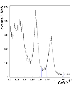
(a) $D_{s}^{+}$

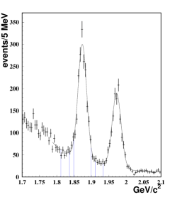
(b) $D^{+}$

Figure 1: Signal and side-band regions of the three-pion invariant-mass distribution for a) $D_{s}^{+}$ and b) $D^{+}$ Dalitz-plot analysis respectively.

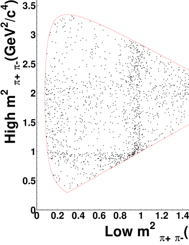
(a) $D_{s}^{+}$

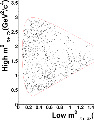
(b) $D^{+}$

Figure 2: a) $D_{s}^{+}$ and b) $D^{+}$ Dalitz plots.

3 The decay amplitude

The decay amplitude of the $D$ meson into the three-pion final state is written as:

$$A(D)=a_{0}e^{i\delta_{0}}+F_{1}+\sum_{i}a_{i}e^{i\delta_{i}}B(abc|r_{i}),$$ (1)

where the first term represents the direct non-resonant three-body amplitude contribution, $F_{1}$ is the contribution of $S$-wave states and the sum is over the contributions from the intermediate two-body non-scalar resonances. $B(abc|r_{i})$ are the usual Breit-Wigner terms of the traditional isobar model, whose explicit forms are given in [9]. $F_{1}$ is written in the context of the K-matrix approach which we will discuss shortly. The coefficients and phases of the $A(D)$ amplitude are all relative to a free parameter of the $F_{1}$ amplitude, $\beta_{1}$, whose modulus and phase are fixed to 1 and 0 respectively (see below). The squared modulus of this amplitude gives the probability density in the three pion Dalitz plot.

In general, the decay of a $D$ meson into three pions via a resonance involves the production of a $(IJ)^{PC}$ state with an accompanying pion. It is believed that, while the usual Breit-Wigner (BW) approximation is suitable for states with $J>0$, since they are characterized by relatively narrow and isolated resonances, the treatment of $S$-wave states requires a more general formalism to account for non-trivial dynamics due to the presence of broad and overlapping resonances [1, 2]. For $J=0$, only states with even isospin and positive $P$ and $C$ are allowed to strongly couple to $\pi^{+}\pi^{-}$. We limit ourselves to isoscalar $S$-wave states, $(00)^{++}$, since $I=2$ must involve at least two $q\bar{q}$ pairs and no four-quark states with $I=2$ are known. At the mass scales relevant to this analysis, the decay of a charm particle into a $(00)^{++}$ state with an accompanying pion consists of five channels $l=1\dots 5$ where $1=\pi\pi$, $2=K\bar{K}$, $3=\mbox{multi-meson}$ states (four-pion state mainly at $\sqrt{s}<1.6\,$GeV) $4=\eta\eta$ and $5=\eta\eta^{\prime}$. The amplitude for the particular channel $(00)^{++}_{l}\pi$ can be written in the context of the K-matrix formalism as

$$F_{l}=(I-iK\rho)_{lj}^{-1}P_{j}\,,$$ (2)

where $I$ is the identity matrix, $K$ is the K-matrix describing the isoscalar $S$-wave scattering process, $\rho$ is the phase-space matrix for the five channels, and $P$ is the “initial” production vector into the five channels. In this picture, the production process can be viewed as consisting of an initial preparation of several states, which are then propagated by the $(I-iK\rho)^{-1}$ term into the final one. Only the $F_{1}$ amplitude is present in the isosinglet $S$-wave term since we are describing the dipion channel.

We require a reliable K-matrix parametrization of $(00)^{++}$-wave scattering. To our knowledge the only self-consistent description of the $S$-wave isoscalar scattering is given by the K-matrix representation of Anisovich and Sarantsev in reference [7] obtained through a global fit of the available scattering data from $\pi\pi$ threshold up to $1900\,$MeV. Their K-matrix parametrization is:

$$K_{ij}^{00}(s)=\left\{\sum_{\alpha}\frac{g^{(\alpha)}_{i}g^{(\alpha)}_{j}}{m^{2}_{\alpha}-s}+f^{\mathrm{scatt}}_{ij}\frac{1\,\mathrm{GeV}^{2}-s_{0}^{\mathrm{scatt}}}{s-s_{0}^{\mathrm{scatt}}}\right\}\frac{(s-s_{A}m^{2}_{\pi}/2)(1-s_{A0})}{(s-s_{A0})}.$$ (3)

The $g^{(\alpha)}_{i}$ is the coupling constant of the K-matrix pole $m_{\alpha}$ to the $i$ meson channel; the parameters $f^{\mathrm{scatt}}_{ij}$ and $s_{0}^{\mathrm{scatt}}$ describe a slowly varying part (which we will call SVP) of the K-matrix elements; the factor $\frac{(s-s_{A}m^{2}_{\pi}/2)(1-s_{A0})}{(s-s_{A0})}$ is to suppress false kinematical singularity in the physical region near the $\pi\pi$ threshold (Adler zero). The parameter values used in this paper are listed in Table 1, which was provided by the authors of reference [7]. Note that K-matrix representation is by definition real and symmetric.

Table 1: K-matrix parameters. Masses and coupling constants are in GeV. Only the $i=1$ $f_{ij}$ terms are reported here since they are the only values relevant to the three-pion decay.

$\begin{array}[]{cccccc}\hline\cr m_{\alpha}&g_{\pi\pi}&g_{K\bar{K}}&g_{4\pi}&g_{\eta\eta}&g_{\eta\eta^{\prime}}\\ \hline\cr 0.65100&0.24844&-0.52523&\,\,0.00000&-0.38878&-0.36397\\ 1.20720&0.91779&\,\,0.55427&\,\,0.00000&\,\,0.38705&\,\,0.29448\\ 1.56122&0.37024&\,\,0.23591&\,\,0.62605&\,\,0.18409&\,\,0.18923\\ 1.21257&0.34501&\,\,0.39642&\,\,0.97644&\,\,0.19746&\,\,0.00357\\ 1.81746&0.15770&-0.17915&-0.90100&-0.00931&\,0.20689\\ \hline\cr s_{0}^{\mathrm{scatt}}&f^{\mathrm{scatt}}_{11}&f^{\mathrm{scatt}}_{12}&f^{\mathrm{scatt}}_{13}&f^{\mathrm{scatt}}_{14}&f^{\mathrm{scatt}}_{15}\\ -3.30564&0.26681&0.16583&-0.19840&0.32808&0.31193\\ \hline\cr s_{A}&s_{A0}&&&&\\ 1.0&-0.2&&&&\\ \hline\cr\end{array}$

The K-matrix values of Table 1 generate a physical T-matrix, $T=(I-iK\cdot\rho)^{-1}K$, which describes the scattering in the $(00)^{++}$-wave with five poles, whose masses, half-widths, and couplings are listed in Table 2.

Table 2: T-matrix poles and $\pi^{+}\pi^{-}$ scattering coupling-constants; phases are in degrees. The $f_{0}(980)$ pole position is found by the authors of [7] on the second Riemann sheet, thus the closest physical region is the beginning of $K\bar{K}$ threshold.

T-matrix pole	$g_{K\mathchoice{\makebox[0.0pt][l]{$\displaystyle\kern 1.435pt\overline{\kern-1.67418pt\phantom{K}\kern-0.3014pt}$}}{\makebox[0.0pt][l]{$\textstyle\kern 1.435pt\overline{\kern-1.67418pt\phantom{K}\kern-0.3014pt}$}}{\makebox[0.0pt][l]{$\scriptstyle\kern 1.0045pt\overline{\kern-1.17192pt\phantom{K}\kern-0.21098pt}$}}{\makebox[0.0pt][l]{$\scriptscriptstyle\kern 0.7175pt\overline{\kern-0.83708pt\phantom{K}\kern-0.1507pt}$}}K}/g_{\pi\pi}$	$g_{4\pi}/g_{\pi\pi}$	$g_{\eta\eta}/g_{\pi\pi}$	$g_{\eta\eta^{\prime}}/g_{\pi\pi}$
( $m,\Gamma/2$ ) GeV
$f_{0}(980)$
(1.019, 0.038)	1.3970 ei83.4	0.3572 ei67.8	1.1660 ei85.5	0.9662 ei89.0
$f_{0}(1300)$
(1.306, 0.170)	0.2579 e-i16.6	2.1960 e-i178.7	0.3504 ei23.2	0.5547 ei16.2
$f_{0}(1200-1600)$
(1.470, 0.960)	1.1140 e-i0.4	2.2200 e-i6.8	0.569 ei17.7	0.2309 ei54.6
$f_{0}(1500$)
(1.488, 0.058)	0.5460 e-i1.8	1.9790 ei85.3	0.4083 ei37.9	0.4692 ei74.6
$f_{0}(1750)$
(1.746, 0.160)	0.1338 ei32.6	1.3680 ei134.8	0.2979 ei25.1	0.5843 e-i0.5

The $f_{0}$ series reported in Table 2 differs somewhat from that reported by the PDG [10] group. In addition to the $f_{0}(980)$ and $f_{0}(1500)$ poles which also appear in the PDG classification, three other poles are present, $f_{0}(1300)$, $f_{0}(1200-1600)$ and $f_{0}(1750)$, in contrast with only two poles listed by the PDG, $f_{0}(1370)$ and $f_{0}(1710)$. The five-pole series used here is able to consistently reproduce the available $S$-wave isoscalar data in the energy range relevant for this analysis. The decay amplitude for the $D$ meson into the three-pion final state, where $\pi^{+}\pi^{-}$ are in a $(IJ^{PC}=00^{++}$)-wave is then

$$F_{1} = (I-iK\rho)^{-1}_{1j}\left\{\sum_{\alpha}\frac{\beta_{\alpha}g_{j}^{(\alpha)}}{m^{2}_{\alpha}-s}+f_{1j}^{\mathrm{prod}}\frac{1\,\mathrm{GeV}^{2}-s_{0}^{\mathrm{prod}}}{s-s_{0}^{\mathrm{prod}}}\right\}$$ (4)

$$\hskip 160.00024pt\hbox{}\times\frac{(s-s_{A}m^{2}_{\pi}/2)(1-s_{A0})}{(s-s_{A0})}\,,$$

where $\beta_{\alpha}$ is the coupling to the $m_{\alpha}$ pole in the ‘initial’ production process, $f_{1j}^{\mathrm{prod}}$ and $s_{0}^{\mathrm{prod}}$ are the P-vector SVP parameters. $\beta_{\alpha}$ and $f_{1j}^{\mathrm{prod}}$ are in general complex numbers [4]. The phase space matrix elements for the two pseudoscalar-particle states are:

$$\rho_{i}(s) = \sqrt{\left(1-\frac{(m_{1i}+m_{2i})^{2}}{s}\right)\left(1-\frac{(m_{1i}-m_{2i})^{2}}{s}\right)}$$ (5)

$$\hskip 160.00024pt(i=\pi\pi,K\bar{K},\eta\eta,\eta\eta^{\prime}).$$

The normalization is such that $\rho_{i}\to 1$ as $s\to\infty$. The expression for the multi-meson state phase space can be found in reference [7].

We note that the P-vector poles have to be the same as those of the K-matrix in order to cancel out infinities in the final amplitude as each pole is realized. The P-vector SVP parametrization is chosen in complete analogy with that used for the K-matrix. The need for the Adler-zero term, not a-priori required in the P-vector, will be investigated by studying its effect on the quality of the fit to our data. The K-matrix parameters are fixed to the values of Table 1 in our Dalitz plot fits. The free parameters are the P-vector parameters ($\beta_{\alpha}$, $f^{\mathrm{prod}}_{1j}$ and $s_{0}^{\mathrm{prod}}$), and the coefficients and phases of Eq. 1 ($a_{0},a_{i}$ and $\delta_{0},\delta_{i}$). All amplitudes are referenced to $\beta_{1}$ which is fixed at 1. The P-vector Adler-zero parameters have been chosen to be identical to those of the K-matrix, $s_{A}$ and $s_{A0}$. Because of the limited allowed range for these parameters, we do not expect our results to critically depend on this particular choice.

4 The likelihood function and fitting procedure

The probability density function is corrected for geometrical acceptance and reconstruction efficiency. We find that finite-mass resolution effects are negligible. The shape of the background in the signal region is parametrized through a polynomial fit to the Dalitz plot of mass sidebands. The number of background events expected in the signal region is estimated through fits to the $\pi^{+}\pi^{-}\pi^{+}$ mass spectrum. All background parameters are included as additional fit parameters and tied to the results of the sideband fits through the inclusion in the likelihood of a $\chi^{2}$ penalty term derived from the covariance matrix of the sideband fit. The contamination in the $D^{+}$ left sideband from $D^{+}\to K^{-}\pi^{+}\pi^{+}$, where $K^{-}$ is misidentified as $\pi^{-}$, is reduced to a negligible level (3.5 % of the total events in the sideband) using the tight Čerenkov cut. Background from the decay, $D_{s}^{+}\to\eta^{\prime}\pi^{+}$ with $\eta^{\prime}\to\rho\gamma$ and $\rho\to\pi^{+}\pi^{-}$, is expected in the $D^{+}$ signal and sideband regions. It is included by adding a $\rho$-BW component in the background parametrization. The $D^{+}$ and $D_{s}^{+}$ samples are fitted with likelihood functions $\mathcal{L}$ consisting of signal and background probability densities. Checks for fitting procedure are made using Monte Carlo techniques and all biases are found to be small compared to the statistical errors. The systematic errors on our results are evaluated by comparing their values in disjoint samples corresponding to different experimental running conditions, different kinematical regions, such as low versus high $D$ momenta, and particle versus anti-particle. A split sample systematic error was added in quadrature to the existing statistical error to make the split sample estimates consistent to within $1\,\sigma$ if necessary. The assumption that the shape of the background in the sideband is a good representation of the background in the signal region could potentially constitute another source of systematic error. We study this effect by varying the polynomial function degree and adding/removing the Breit-Wigner terms, which are introduced to take into account any feed-through from resonances in the background, and computing the r.m.s. of the different results, which is added in quadrature to form the total experimental systematic error.

5 Results for the $D^{+}_{s}\to\pi^{+}\pi^{-}\pi^{+}$ decay

We recall that the physical parameters of our fit are P-vector parameters: $\beta_{\alpha}$, $f^{\mathrm{prod}}_{1j}$, along with $s_{0}^{\mathrm{prod}}$, and the coefficients and phases of Eq. 1, $a_{0},a_{i}$ and $\delta_{0},\delta_{i}$. The K-matrix parameters are fixed to the values given in Table 1. The general procedure, adopted for all the fits reported here, consists of several successive steps in order to eliminate contributions whose effects on our fit are marginal. We initially consider all the well established, non-scalar resonances decaying to $\pi^{+}\pi^{-}$ with a sizeable branching ratio. Contributions are removed if their amplitude coefficients, $a_{i}$ of Eq. 1, are less than $2\,\sigma$ significant and the fit confidence level increases due to the decreased number of degrees of freedom in the fit. The P-vector initial form includes the complete set of K-matrix poles and slowly varying function (SVP) as given in reference [7]; $\beta_{\alpha}$ as well as the $f^{\mathrm{prod}}_{1j}$ terms of Eq. 4 are removed with the same criteria. The fit confidence levels (C.L.) are evaluated with a $\chi^{2}$ estimator over a Dalitz plot with bin size adaptively chosen to maintain a minimum number of events in each bin. Once the minimal set of parameters is reached, addition of each single contribution previously eliminated is reinstated to verify that the C.L. does not improve.

Table 3 shows the P-vector composition from our final fit results on the $D_{s}^{+}\to\pi^{+}\pi^{-}\pi^{+}$ Dalitz plot.

Table 3: P-vector parameters of the $D_{s}^{+}$ fit.

P-vector parameters	modulus	phase (deg)
$\beta_{1}$	1 (fixed)	0 (fixed)
$\beta_{2}$	$0.974\pm 0.102$	$207.0\pm 5.9$
$\beta_{3}$	$0.755\pm 0.196$	$\,\,\,85.7\pm 19.3$
$\beta_{4}$	$1.760\pm 0.371$	$119.1\pm 19.9$
$f^{\mathrm{prod}}_{11}$	$0.863\pm 0.153$	$202.3\pm 9.4$
$f^{\mathrm{prod}}_{13}$	$3.768\pm 0.746$	$140.3\pm 16.7$
$f^{\mathrm{prod}}_{14}$	$2.179\pm 0.663$	$106.6\pm 24.4$
$f^{\mathrm{prod}}_{15}$	$2.452\pm 0.684$	$236.5\pm 13.7$

The fifth K-matrix pole and the second SVP contribution were eliminated. The inclusion of an Adler zero term did not improve our fit quality and was removed. The quoted results were obtained with $s^{\mathrm{prod}}_{0}=-3$ GeV², but they were insensitive to any choice in the range $-5\,$GeV${}^{2}\leq s^{\mathrm{prod}}_{0}\leq-1\,$GeV² – typical parameter values for the SVP.

The resulting fit fractions , phases and amplitude coefficients are quoted in Table 4. We note that both the three-body non-resonant and $\rho^{0}(770)\pi^{+}$ components were not required by the fit. We represent the entire $S$-wave contribution by a single fit fraction since, as previously discussed, one cannot distinguish the different resonance or SVP $S$-wave contributions on the real axis. The couplings to T-matrix physical poles, reported in Table 5, are computed by continuing the amplitude $F_{1}(s)$ into the complex s-plane to the position of the poles and evaluating the pole residues . The $D_{s}^{+}$ Dalitz projections of our data are shown in Fig. 3 superimposed with our final fit projections. Figure 4 shows the corresponding adaptive binning scheme used to obtain the fit confidence level.

Table 4: Fit results from the K-matrix model for $D_{s}^{+}$.

decay channel	fit fraction (%)	phase (deg)	amplitude coefficient
($S$-wave) $\pi^{+}$	$87.04\pm 5.60\pm 4.17$	0 (fixed)	1 (fixed)
$f_{2}(1270)\,\pi^{+}$	$9.74\pm 4.49\pm 2.63$	$168.0\pm 18.7\pm 2.5$	$0.165\pm 0.033\pm 0.032$
$\rho^{0}(1450)\,\pi^{+}$	$6.56\pm 3.43\pm 3.31$	$234.9\pm 19.5\pm 13.3$	$0.136\pm 0.030\pm 0.035$
Fit C.L	3.0 %

Table 5: $D_{s}^{+}\to\pi^{+}\pi^{-}\pi^{+}$ production coupling constants for the five T-matrix poles, which comprise the $S$-wave component in Table 4, referenced to the $f_{0}(980)$. Phases are in degrees.

T-matrix pole	($m,\Gamma/2$) (GeV)	$D_{s}^{+}$ (relative) coupling constant
$f_{0}(980)$	(1.019, 0.038)	1 ei0 (fixed)
$f_{0}(1300)$	(1.306, 0.170)	$(0.43\pm 0.04)$ ei(-163.8±4.9)
$f_{0}(1200-1600)$	(1.470, 0.960)	$(4.90\pm 0.08)$ ei(   80.9±1.06)
$f_{0}(1500)$	(1.488, 0.058)	$(0.51\pm 0.02)$ ei(   83.1±3.03)
$f_{0}(1750)$	(1.746, 0.160)	$(0.82\pm 0.02)$ ei(-127.9±2.25)

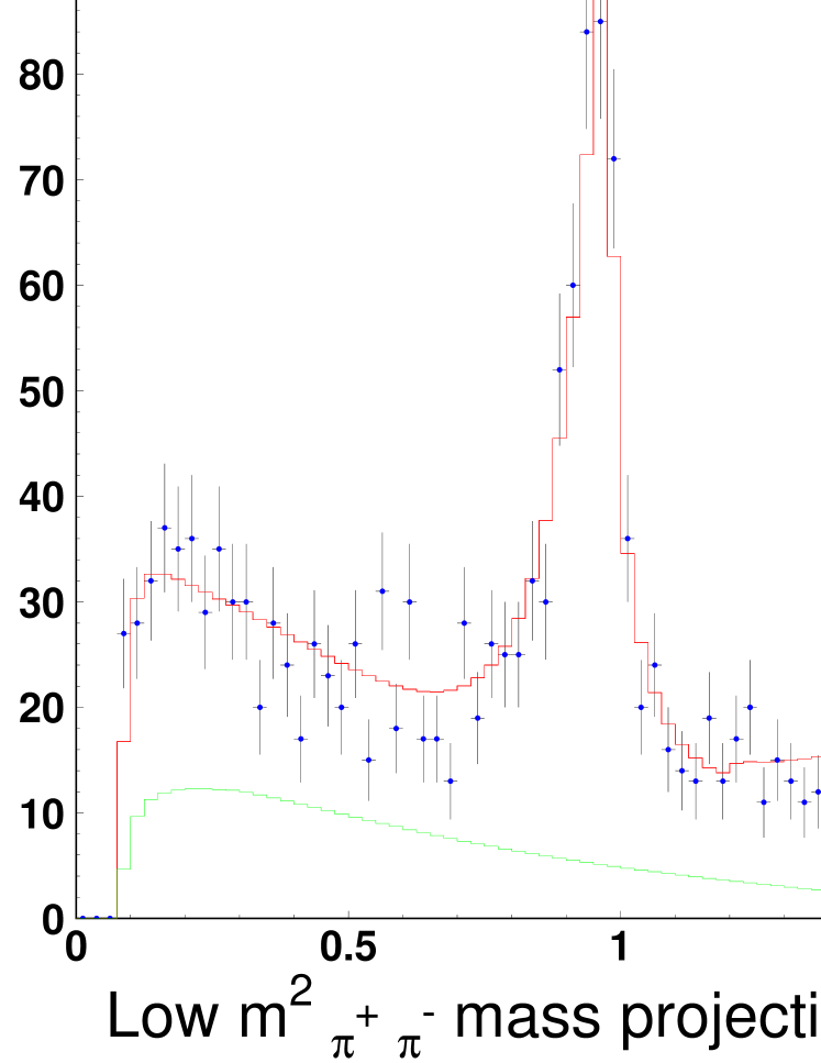
Figure 3: $D_{s}^{+}$ Dalitz-plot projections with our final fit superimposed. The background shape under the signal is also shown.

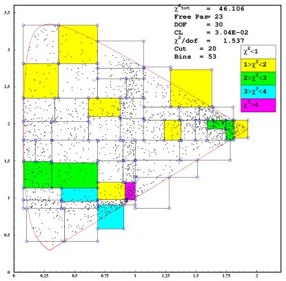
Figure 4: $D_{s}^{+}$ adaptive binning Dalitz-plot for the K-matrix model.

6 Results for the $D^{+}\to\pi^{+}\pi^{-}\pi^{+}$ decay

The $D^{+}\to\pi^{+}\pi^{-}\pi^{+}$ Dalitz plot shows an excess of events at low $\pi^{+}\pi^{-}$ mass, which cannot be explained in the context of the simple isobar model with the usual mixture of well established resonances along with a constant, non-resonant amplitude. A new scalar resonance, the $\sigma(600)$, has been previously proposed [11] to describe this excess. However we know that complex structure can be generated by the interplay among the $S$-wave resonances and the underlying non-resonant $S$-wave component that cannot be properly described in the context of a simple isobar model. It is therefore interesting to study this channel with the present formalism, which embeds all our experimental knowledge about the $S$-wave $\pi^{+}\pi^{-}$ scattering dynamics.

With the same procedure based on statistical significance and fit confidence level used in the $D_{s}^{+}$ analysis, we obtained the final set of P-vector parameters that is reported in Table 6.

Table 6: P-vector parameters of the $D^{+}$ fit.

P-vector parameters	modulus	phase (deg)
$\beta_{1}$	1 (fixed)	0 (fixed)
$\beta_{2}$	$2.471\pm 0.431$	$82.5\pm 10.3$
$\beta_{3}$	$1.084\pm 0.386$	$102.8\pm 23.5$
$f^{\mathrm{prod}}_{11}$	$2.565\pm 0.737$	$155.4\pm 18.3$
$f^{\mathrm{prod}}_{12}$	$6.312\pm 0.967$	$-160.0\pm 8.7$

The last two poles and the last three SVP terms were eliminated. The $s^{\mathrm{prod}}_{0}$ value is measured to be $s^{\mathrm{prod}}_{0}=(-1.0^{+0.4}_{-5.5})\,$GeV² . The fit did not require an Adler-zero term.

Beside the $S$-wave component, the decay appears to be dominated by the $\rho^{0}(770)$ plus a $f_{2}(1270)$ component. The $\rho^{0}(1450)$ was always found to have less than $2\,\sigma$ significance and was therefore dropped from the final fit. In analogy with the $D_{s}^{+}$, the direct three-body non-resonant component was not necessary since the SVP of the $S$-wave could reproduce the entire non-resonant portion of the Dalitz plot. The complete fit results are reported in Table 7. The resulting production coupling constants are reported in Table 8.

Table 7: Fit results from the K-matrix model fit for $D^{+}$.

decay channel	fit fraction (%)	phase (deg)	amplitude coefficient
($S$-wave) $\pi^{+}$	$56.00\pm 3.24\pm 2.08$	0 (fixed)	1 (fixed)
$f_{2}(1270)\,\pi^{+}$	$11.74\pm 1.90\pm 0.23$	$-47.5\pm 18.7\pm 11.7$	$1.147\pm 0.291\pm 0.047$
$\rho^{0}(770)\,\pi^{+}$	$30.82\pm 3.14\pm 2.29$	$-139.4\pm 16.5\pm 9.9$	$1.858\pm 0.505\pm 0.033$
Fit C.L.	7.7 %

Table 8: $D^{+}\to\pi^{+}\pi^{-}\pi^{+}$ production coupling constants for the five T-matrix poles, which comprise the $S$-wave component in Table 7, referenced to the $f_{0}(980)$. Phases are in degrees.

T-matrix pole	($m,\Gamma/2$) (GeV)	$D^{+}$ (relative) coupling constant
$f_{0}(980)$	(1.019, 0.038)	1 ei0 (fixed)
$f_{0}(1300)$	(1.306, 0.170)	$(0.67\pm 0.03)$ ei(-67.9±3.0)
$f_{0}(1200-1600)$	(1.470, 0.960)	$(1.70\pm 0.17)$ ei(-125.5±1.7)
$f_{0}(1500)$	(1.488, 0.058)	$(0.63\pm 0.02)$ ei(-142.2±2.2)
$f_{0}(1750)$	(1.746, 0.160)	$(0.36\pm 0.02)$ ei(-135.0±2.9)

The $D^{+}$ Dalitz projections are shown in Fig. 5 and the corresponding adaptive binning scheme is shown in Fig. 6.

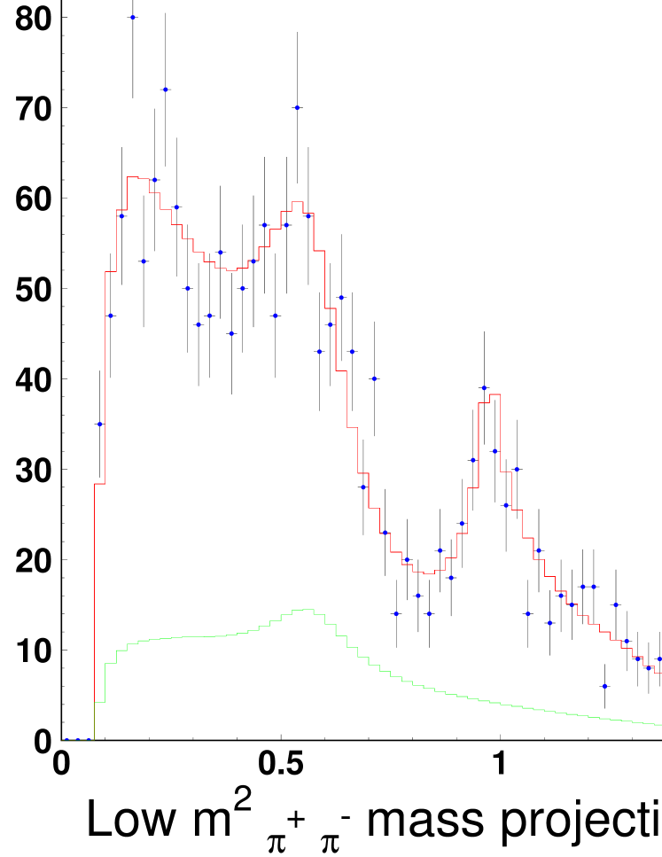
Figure 5: $D^{+}$ Dalitz-plot projections with our final fit superimposed. The background shape under the signal is also shown.

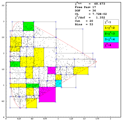
Figure 6: $D^{+}$ adaptive binning Dalitz-plot for the K-matrix fit.

The most interesting feature of these results is the fact that the better treatment of the $S$-wave contribution provided by the K-matrix model can reproduce the low-mass $\pi^{+}\pi^{-}$ structure of the $D^{+}$ Dalitz plot. This suggests that any $\sigma$-like object in the $D$ decay should be consistent with the same $\sigma$-like object measured in the $\pi^{+}\pi^{-}$ scattering. We believe that additional studies with higher statistics will be required to completely understand the $\sigma$ puzzle.

7 $D_{s}^{+}$ and $D^{+}$ final results

The K-matrix parameters used in this analysis correspond to the best solution provided by the authors of reference [7]. Several solutions with slightly different parametrizations for the 4$\pi$ phase-space and for the K-matrix background terms were presented in the same paper. We evaluate the systematic error due to solution choice by computing the r.m.s. of the fit fractions and phases obtained using the different solutions. The final results, including this last systematic error, are presented in Table 9.

Table 9: Final results on $D_{s}^{+}$ and $D^{+}\to\pi^{+}\pi^{-}\pi^{+}$ fit fractions and phases. Beside the first reported error, which is statistical, two systematic errors are quoted. The first one is from the measurement systematics and the second one is due to the particular solution chosen for the K-matrix poles and backgrounds.

$D_{s}^{+}$
decay channel	fit fraction (%)	phase (deg)
($S$-wave) $\pi^{+}$	$87.04\pm 5.60\pm 4.17\pm 1.34$	0 (fixed)
$f_{2}(1270)\,\pi^{+}$	$9.74\pm 4.49\pm 2.63\pm 1.32$	$168.0\pm 18.7\pm 2.5\pm 21.7$
$\rho^{0}(1450)\pi^{+}$	$6.56\pm 3.43\pm 3.31\pm 2.90$	$234.9\pm 19.5\pm 13.3\pm 24.9$
$D^{+}$
decay channel	fit fraction (%)	phase (deg)
($S$-wave) $\pi^{+}$	$56.00\pm 3.24\pm 2.08\pm 0.50$	0 (fixed)
$f_{2}(1270)\,\pi^{+}$	$11.74\pm 1.90\pm 0.23\pm 0.18$	$-47.5\pm 18.7\pm 11.7\pm 5.3$
$\rho^{0}(770)\pi^{+}$	$30.82\pm 3.14\pm 2.29\pm 0.17$	$-139.4\pm 16.5\pm 9.9\pm 5.0$

8 Conclusions

The K-matrix formalism has been applied for the first time to the charm sector in our Dalitz plot analyses of the $D_{s}^{+}$ and $D^{+}\to\pi^{+}\pi^{-}\pi^{+}$ final states. The results are extremely encouraging since the same K-matrix description gives a coherent picture of both two-body scattering measurements in light-quark experiments as well as charm meson decay. This result was not obvious beforehand. Furthermore, the same model is able to reproduce features of the $D^{+}\to\pi^{+}\pi^{-}\pi^{+}$ Dalitz plot that otherwise would require an ad hoc $\sigma$ resonance. In addition, the non-resonant component of each decay seems to be described by known two-body $S$-wave dynamics without the need to include constant amplitude contributions.

The K-matrix treatment of the $S$-wave component of the decay amplitude allows for a direct interpretation of the decay mechanism in terms of the five virtual channels considered: $\pi\pi$, $K\bar{K}$, $\eta\eta$, $\eta\eta^{\prime}$ and $4\,\pi$. By inserting $KK^{-1}$ in the decay amplitude, $F$,

$$F=(I-iK\rho)^{-1}P=(I-iK\rho)^{-1}KK^{-1}P=TK^{-1}P=TQ$$ (6)

we can view the decay as consisting of an initial production of the five virtual states which then scatter via the physical $T$ into the final state. The Q-vector contains the production amplitude of each virtual channel in the decay. Figure 7 shows the ratio of the moduli of the Q-vector amplitudes with respect to the $\pi\pi$ modulus for the $D_{s}^{+}$ $S$-wave. The last plot in Fig. 7 represents the normalizing $\pi\pi$ modulus. The two peaks of the ratios correspond to the two dips of the $\pi\pi$ normalizing modulus, while the two peaks due to the K-matrix singularities, visible in the normalization plot, cancel out in the ratios.

Figure 7: Measured $D_{s}^{+}$ Q-vector components: the first four plots are the ratios of moduli of the Q-vector amplitudes with respect to the $\pi\pi$ modulus; the last plot is the normalizing $\pi\pi$ modulus.

Figure 8 shows the analogous plots for the $D^{+}$ $S$-wave decay. The resulting picture, for both $D_{s}^{+}$ and $D^{+}$ decay, is that the $S$-wave decay is dominated by an initial production of $\eta\eta$, $\eta\eta^{\prime}$ and $K\bar{K}$ states. Dipion production is always much smaller. This suggests that in both cases the $S$-wave decay amplitude primarily arises from a $s\bar{s}$ contribution such as that produced by the Cabibbo favoured weak diagram for the $D_{s}^{+}$ and one of the two possible singly Cabibbo suppressed diagrams for the $D^{+}$. For the $D^{+}$, the $s\bar{s}$ contribution competes with a $d\bar{d}$ contribution. That the $f_{0}(980)$ appears as a peak in the $\pi\pi$ mass distribution in $D^{+}$ decay, as it does in $D_{s}$ decay, shows that for the $S$-wave component the $s{\bar{s}}$ contribution dominates [2]. Comparing the relative $S$-wave fit fractions that we observe for $D_{s}^{+}$ and $D^{+}$ reinforces this picture. The $S$-wave decay fraction for the $D_{s}^{+}$ (87 %) is larger than that for the $D^{+}$ (56 %). Rather than coupling to an $S$-wave dipion, the $d\bar{d}$ piece prefers to couple to a vector state like $\rho^{0}(770)$ that alone accounts for $\sim 30\,\%$ of $D^{+}$ decay.

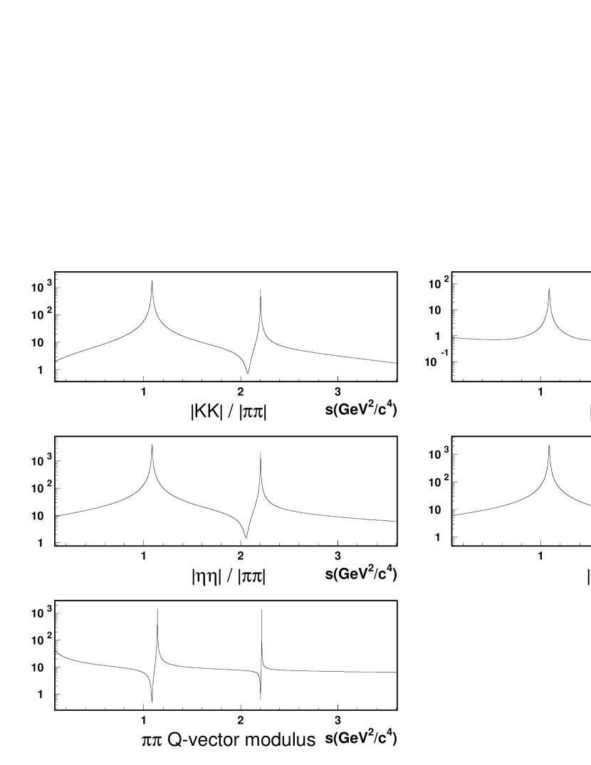
Figure 8: Measured $D^{+}$ Q-vector components: the first four plots are the ratios of moduli of the Q-vector amplitudes with respect to the $\pi\pi$ modulus; the last plot is the normalizing $\pi\pi$ modulus.

This interpretation also bears on the role of the annihilation diagram in the $D_{s}^{+}\to\pi^{+}\pi^{-}\pi^{+}$ decay. We believe that Fig. 7 suggests that the $S$-wave annihilation contribution is negligible over much of the dipion mass spectrum. It might be interesting to search for annihilation contributions in higher spin channels, such as $\rho^{0}(1450)\pi$ and $f_{2}(1270)\pi$.

9 Acknowledgments

We are particularly indebted to Prof. M. R. Pennington, for his patience in guiding us through the fascinating K-matrix world and for his frequent advice in formalizing our problem. This work would have not be possible without the invaluable help and assistance by Prof. V. V. Anisovich and Prof. A. V. Sarantsev, who provided us with K-matrix input numbers and even crucial pieces of code. Their expertise was vital to us and certainly accelerated our work. We wish to acknowledge the assistance of the staffs of Fermi National Accelerator Laboratory, the INFN of Italy, and the physics departments of the collaborating institutions. This research was supported in part by the US National Science Fundation, the US Department of Energy, the Italian Istituto Nazionale di Fisica Nucleare and Ministero dell’Istruzione dell’Università e della Ricerca, the Brazilian Conselho Nacional de Desenvolvimento Científico e Tecnológico, CONACyT-México, the Korean Ministry of Education, and the Korean Science and Engineering Foundation.

References

- [1] S. Spanier and N. A. Törnqvist, Scalar Mesons (rev.), Particle Data Group, Phys. Rev. D66 (2002) 010001-450.
- [2] M. R. Pennington, Proc. of Oxford Conf. in honour of R. H. Dalitz, Oxford, July, 1990, Ed. by I. J. R. Aitchison, et al., (World Scientific) pp. 66–107; Proc. of Workshop on Hadron Spectroscopy (WHS 99), Rome, March 1999, Ed. by T. Bressani et al., (INFN, Frascati).
- [3] E. P. Wigner, Phys. Rev. 70 (1946) 15.
- [4] S. U. Chung et al., Ann. Physik 4 (1995) 404.
- [5] I. J. R. Aitchison, Nucl. Phys. A189, (1972) 417.
- [6] K. L. Au, D. Morgan, and M. R. Pennington, Phys. Rev. D35 (1987) 1633.
- [7] V. V. Anisovich and A. V. Sarantsev, Eur. Phys. J. A16 (2003) 229.
- [8] J. M. Link et al., Nucl. Instr. Meth. A484 (2002) 270.
- [9] P. L. Frabetti et al., Phys. Lett. B407 (1997) 79.
- [10] Particle Data Group, Phys. Rev. D66 (2002) 010001.
- [11] E. M. Aitala et al., Phys. Rev. Lett. 86 (2001) 770.
- [12] R. N. Chan and P. V. Landshoff, Nucl. Phys. B266 (1986) 451.