KALMAN FILTER BASED TRACKER STUDY FOR $\mu e$ - CONVERSION EXPERIMENT

Abstract

The search for muon to electron conversion with a sensitivity of the order $10^{-17}$ requires a several order of magnitude increase in muon intensity and a high resolution, $\sigma\simeq$ 0.1 MeV/c of the electron’s momentum.

We present results of a pattern recognition and track momentum reconstruction algorithm that relies on a Kalman filter approach. Background from captured protons, neutrons, photons and from muon decay in orbit were generated by GEANT. The effective average straw tube background rate was 800 kHz.

The pattern recognition proceeds in two stages. In the first, simple considerations using only straw tube center coordinates, without drift time information, were applied to reduce the background to a manageable level. Then the drift time information is incorporated and a Deterministic Annealing Filter applied to reach the final level of background suppression and to provide a starting point for the track momentum reconstruction using the Kalman filter. This procedure reduces the simulated background by a factor 800 with small,(2.7%), losses in real tracker hits.

The momentum resolution of the tracker is $\sigma$ = 0.12 MeV/c and the acceptance for muon conversion events with momentum above 103.6 MeV/c is 22%. These numbers do not differ significantly from the values obtained without background.

The expected number of events from muon decay in orbit (main background) in which the decay electron has momentum greater than 100 MeV/c is 0.3, compared to 6.5 $\mu e$ - conversion events above the same threshold for $R_{\mu e}=10^{-16}$.

I Introduction

The observation of $\mu e$ - conversion would provide the first direct evidence for lepton flavor violation in charged lepton sector and require new physics, beyond the Standard Model (see  kuno and references therein). Lepton flavor is not conserved in neutrino oscillations but the modifications to the Standard Model to include the small neutrino masses do not lead to an appreciable rate for $\mu e$ - conversion

$\mu^{-}+N\to e^{-}+N$ .

This process violates the lepton flavor numbers, $L_{e}$ and $L_{\mu}$, but conserves the total lepton number. The signature of the process is very clear: a single monochromatic electron in the final state with the energy close to the muon mass:

$E_{e}=m_{\mu}-B_{\mu}-E_{rec}$

where $m_{\mu}$ is a muon mass, $B_{\mu}$ is a binding energy of the 1s muonic atom, $E_{rec}$ is a nuclear recoil energy.

The SINDRUM II collaboration at PSI has carried out a program of experiments to search for $\mu e$ - conversion in various nuclei. They find that at 90% CL the upper limit for the reaction $\mu^{-}+Ti\to e^{-}+Ti$ is $6.1\times 10^{-13}$  psi . In this experiment muons were accumulated at a rate of $10^{7}\mu^{-}/sec$. According to preliminary results  psigold for the reaction $\mu^{-}+Au\to e^{-}+Au$ a single event sensitivity is $3.3\times 10^{-13}$

In  rashid an idea of increasing of muon beam intensity by a few orders of magnitude up to $10^{11}\mu^{-}/sec$ based on the solenoid-capture scheme was discussed and MELC experiment was proposed  abadj with a goal to reach a sensitivity of the order $10^{-17}$.

A new $\mu e$ - conversion experiment MECO (Muon Electron COnversion) E-940  bnl , exploiting the idea of the solenoid-capture scheme, is under preparation at BNL. MECO aims to search for $\mu^{-}+Al\to e^{-}+Al$ with a single event sensitivity 2$\times$$10^{-17}$. It will use a new high-intensity pulsed muon beam, which could yield about $10^{11}\mu^{-}/sec$ stopped in a target.

Also the PRIME (PRISM MuE conversion) working group at KEK expressed an interest  prime to carry out a search for lepton flavor violation in $\mu e$ - conversion in a muonic atom at a sensitivity of $10^{-18}$ using a proposed high intensity pure muon source of $10^{11}-10^{12}\mu^{-}/sec$ .

In this article we develop a pattern recognition and track reconstruction procedure based on the Kalman filter technique for a transverse version of tracker for MECO experiment.

This paper is organized as follows: In section 2 the transverse tracker is described and the advantages of the tracker discussed. In Section 3 possible backgrounds are discussed and the procedure of background simulation briefly explained. In Section 4 the pattern recognition procedure is developed. At this stage a deterministic annealing filter (DAF) is applied to make a final background suppression and provide a starting point for track momentum reconstruction by the Kalman filter technique. Section 5 describes the procedure of momentum reconstruction based on the Kalman filter. Results of the pattern recognition and momentum reconstruction are presented in this section. A brief summary outlook can be found in Section 6. The appendices provide a more detailed look at Kalman filter and deterministic annealing filter. Also tracker resolution is discussed in Appendix.

II The Transverse Tracker Description

The goal of the MECO tracker is to detect the electron from $\mu e$ - conversion with large acceptance and measure its momentum with high resolution ($\sigma\simeq$ 0.1 MeV/c). The tracker is located in a uniform 1T magnetic field. The minimal tracker length is defined by the following requirements:

Background electrons with an energy around 105 MeV are produced by cosmic rays in the wall between the transport and detector solenoids. These electrons cannot have a pitch angle $\theta$ in the tracker greater than $45^{o}$, due to the adiabatic character of charge particle movement. To suppress the cosmic ray background we require that measured pitch angle $\theta_{min}$ for signal events to be more than $45^{o}$.

To get more redundancy for signal events we require that the measured trajectory should have two full turns. This requirement sets limits on the minimal tracker length, which is expressed as:

$L_{Tracker}^{min}=4\cdot\pi\cdot 1/2.998\cdot P\cdot cos(\theta_{min})/B\simeq 4.19\cdot 105\cdot 0.707$/1.0 $\simeq$ 310 cm

where P is a muon conversion momentum (MeV/c) and B is a magnetic field (1 Tesla) in the tracker region.

The tracker consists of 18 modules spaced 17 cm apart. A module consists of 6 planes, each turned at 30^o and shifted 2.5 cm relative to the previous one (Figure  1). A plane consists of two trapezoidal chambers of width 30 cm and lengths 70 to 130 cm in an up and down configuration. The chamber coordinate systems are defined by a rotation angle proportional to 30^o giving an effective “stereo” of crossed directions for 12 different views.

A protective sheath is used to suppress background Compton electrons from a chamber frame. The protective sheath makes nonsensitive a small region of the anode wire near the frame.

The chamber consists of one layer of straw tubes (60 straws) of 5 mm diameter, and length varying from 70 cm to 130 cm. The total number of chambers is 216. The chamber sensitive area starts from 38 cm radius. The straws are assumed to have wall thickness 15 $\mu$m and are constructed of kapton. The total thickness of each chamber is 9 mg/$cm^{2}$. The total number of the tracker straws is 12960. The tracker length is 302 cm. A signal from the straw anode wire will be used to get drift time.

The Al target is tapered in the downstream direction, with 5 cm disk spacing and radii from 8.3 cm to 6.53 cm. The target is placed in the graded portion of the DS magnetic field, with the first disk at 1.75 T and the last at 1.3 T. Protons from the muon capture are absorbed in three concentric polyethylene absorbers: a conical tube of dimensions $R_{1}$ = 46 cm, $R_{2}$ = 70 cm, L = 260 cm and a tube (R = 70 cm, L = 200 cm) both have thickness 3 mm, and a tube of smaller radius (R = 36 cm, L = 235 cm) of thickness 0.5 mm which are placed before the tracker.

Figure 1: Schematic drawing of the tracker design.

The transverse tracker is to be compared with a longitudinal version that MECO is also considering. The longitudinal tracker  bnl consists of an octagonal array of eight detector planes placed symmetrically around the Detector Solenoid axis, plus eight more planes projecting radially outward from each vertex of the octagon. Each plane consists of resistive straws approximately 300 cm long. A hit position in the radial and azimuthal direction is determined by the straw position and the drift time on the anode wire. The hit position in the axial direction is determined by the centroid of the imaged charge from the anode wire, as collected on cathode pads.

The transverse tracker would have several advantages in comparison with a longitudinal one since:

$\bullet$ Normal non resistive straws are used without a pad system.
$\bullet$ Gas manifolds, straw end-caps and chamber supports are all outside the conversion electron trajectories.
$\bullet$ Shorter straws (0.7 - 1.3 m) are technically easier to build and are more robust against instability than longitudinal straws of 3 m.
$\bullet$ Complications from the small tilt of each plane of the longitudinal tracker with respect to the magnetic field are avoided.
$\bullet$ Transverse geometry provides a simple signature of an event since charged particles cross a single straw only once.
$\bullet$ There is a significant simplification dealing only with single chamber hits points.
$\bullet$ The average number of spatially separated hits is a few times greater in comparison with the number of spatially separated clusters in the longitudinal tracker. The hits are distributed uniformly in lobes along the transverse tracker.
$\bullet$ The transverse tracker presents less material in the case of 15 $\mu$m straw wall thickness. The effective total thickness is 29*(15+2)*3.14 = 1550 $\mu$m versus longitudinal tracker 8*3.5*25*3.14 = 2200 $\mu$m.
$\bullet$ The pattern recognition can be performed with good precision even without drift time and amplitude information.
$\bullet$ The Cu layer covering straw tubes suppresses significantly gas diffusion through a straw wall.
$\bullet$ Capacitive crosstalk between channels is small.
$\bullet$ Low energy Compton electron backgrounds have distinguished signature.

III Background simulation

Our analysis is based on a full GEANT simulation taking into account an individual straw structure. Multiple scattering and energy loss are taken into account. Isobutane ($C_{4}H_{10}$) gas is assumed to fill the tubes.

For the subsequent analysis we take only events satisfying the following criteria: number of hits in the tracker is greater than 15; MC simulated energy release in the calorimeter is greater than 80 MeV; pitch angle is greater than 45 ⁰. That leaves about $35\%$ of the original events.

The primary sources of charged particles in the tracker detector during the detection time are protons, neutrons and photons from muon capture by ${}^{27}Al$ nuclei and electrons from muon decay in orbit. The average and peak tracker rates from different backgrounds are presented in Table   1. The main source of background to muon conversion is muon decay in orbit (DIO).

Table 1: The Average and Peak (in parenthesis) Tracker Rates

Processes	proton	neutron	$\gamma$	DIO	DIO
				$<$ 55 MeV	$>$ 55MeV
Particles/process	0.1	1.2	1.8	0.9945	$5.5\cdot 10^{-3}$
Particles/nsec	$120(170)\times 0.1$	$120(170)\times 1.2$	$120(170)\times 1.8$	80 (115)	80 (115)
Prob. Particle to Hit Tracker	$1.08\cdot 10^{-2}$	$0.92\cdot 10^{-3}$	$0.9\cdot 10^{-3}$	$4.0\cdot 10^{-4}$	$1.4\cdot 10^{-2}$
Events in Tracker/30ns	3.9 (5.5)	4.0 (5.6)	5.9 (8.2)	1.0 (1.4)	0.2 (0.3)
Straws on in Tracker/event	14.0	5.2	31.0	15.7	4.3
Straw Rate (kHz)	140 (200)	53 (75)	470 (650)	40 (56)	2.2 (3.3)

To study the tracker performance in the presence of the background the number of muon conversion events ($10^{5}$) with initial momentum of conversion electrons produced in the target (105 MeV/c) was simulated and saved to a data file. The expected number of DIO events during the experiment time ($10^{7}$ sec) in this region is $5.2\cdot 10^{4}$ events above 100 MeV/c.

To study the main background the number of simulated DIO events in this energy region was chosen to be ten times greater. Five different random backgrounds (protons, neutrons, photons and DIO (see Table  1) were generated and saved to data files.

The numbers in the table are the result of a GEANT simulations at the anticipated beam intensity, with no artificial increase as a safety factor. No suppression was added for rejection of heavy ionization particles.

Background was taken from the data files and added to conversion events and DIO events above 100 MeV/c. For example, we simulate the number of events N for the proton background according to a Poisson distribution with average 3.9 taken from background Table  1. Then we randomly pick-up N accidental proton events from the corresponding data file and add these events to the muon conversion or DIO event. In the same way the above procedure is repeated for all background types.

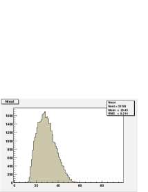
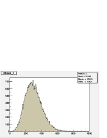
In Figure  2 distributions in the number of real and background tracker hits are shown. The average number of real hits is 29. The real hits distribution starts from 15 hits, corresponding to the cut-off in the minimum number of selected hits. The maximum number of real tracker hits can reach 60. The average number of background hits is 300 which corresponds to an average straw rate about 800 kHz. The distribution in the number of background hits is a broad one and the maximum number of hits is about 900.

Figure 2: Distributions in the number of real and background tracker hits.

IV Pattern recognition

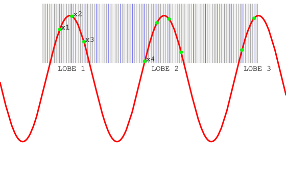
There are twelve views in the tracker, each separated from the previous by 30 degrees. In a typical event, a two-dimensional projection of the helical trajectory, a sine curve, is observed in three or four of the views. There are approximately 10 hits in each view, and 29 hits in the event. The hits are grouped in lobes (see Figure  3) with a typical gap between lobes about 60 cm (in these gaps an electron travels in vacuum). Therefore in the sensitive area of the tracker one gets track segments but not a complete track and the problem of combining information from different lobes arises. Since in a given view at least 4 hits are required to reconstruct four parameters describing a two-dimensional projection of helix often it is not possible to get helix parameters for a track segment in a single lobe and than to apply track element merging strategy. Quite opposite one has to use hits from different lobes for pattern recognition and then for momentum reconstruction. We will show that an appropriate mathematical approach allows to resolve the problem..

The sinusoidal projection of helix is described by four parameters: $x_{0}^{\prime}$ , $z_{0}^{\prime}$, $R_{L}$, $R_{T}$,

$$x_{i}^{\prime}=x_{0}^{\prime}+R_{T}\cos(\frac{z_{i}-z_{0}^{\prime}}{R_{L}})$$ (1)

where importantly, $R_{L}$ and $R_{T}$, related to the longitudinal and transversal momenta, and z coordinate are common to all projections. Coordinate $x^{\prime}$ is defined in a system for each given view.

A simple and powerful reconstruction strategy starts from a single chamber view. To determine the parameters in this view a minimum of four hits are required. The total momentum and momentum pitch angle are determined.

Figure 3: Lobes in the tracker.

To find the five parameters describing the full 3-dimensional helix, one additional hit outside the plane is required:

$$x_{i}^{\prime}=x_{0}^{\prime}+R_{T}\cos(\frac{z_{i}-z_{0}^{\prime}}{R_{L}});~{}~{}~{}~{}~{}~{}~{}y_{i}^{\prime}=y_{0}^{\prime}+R_{T}\sin(\frac{z_{i}-z_{0}^{\prime}}{R_{L}})$$ (2)

The mathematical procedure to find the parameters is the following one:

$\bullet$ four hits from a single view are taken to give the system of equations for helix parameters in the coordinate system related with the view.
$\bullet$ the system of four equations is reduced to a unique equation for $R_{L}$.

$$\Delta x_{24}S_{43}S_{41}S_{31}+\Delta x_{14}S_{43}S_{42}S_{23}+\Delta x_{34}S_{41}S_{42}S_{12}=0$$ (3)

where $\Delta x_{ij}=x_{i}^{\prime}-x_{j}^{\prime}$ , $S_{ij}=\sin((z_{i}-z_{j})/2R_{L}).$
$\bullet$ the equation is solved for $R_{L}$ numerically by the Newton-Raphson method.
$\bullet$ the parameters are expressed in terms of $R_{L}$.

$$\tan(z_{0}^{\prime}/R_{L})=\frac{\Delta x_{14}S_{43}\sin((z_{4}+z_{3})/2R_{L})-\Delta x_{34}S_{41}\sin((z_{4}+z_{1})/2R_{L})}{\Delta x_{14}S_{43}\cos((z_{4}+z_{3})/2R_{L})-\Delta x_{34}S_{41}\cos((z_{4}+z_{1})/2R_{L})}$$ (4)

$$R_{T}=\frac{\Delta x_{12}}{c_{1}-c_{2}}$$

$$x_{0}^{\prime}=\frac{x_{2}c_{1}-x_{1}c_{2}}{c_{1}-c_{2}}$$

where $c=\cos((z_{i}-z_{0}^{\prime})/R_{L}).$

$\bullet$ a fifth hit from a different view is included to obtain the remaining parameters of helix.

$$x_{0}=\frac{1}{\sin(\alpha^{\prime\prime}-\alpha^{\prime})}\left\{x_{0}^{\prime}\sin\alpha^{\prime\prime}-[x_{5}^{\prime\prime}-R_{T}\cos(\frac{z_{5}-z_{0}}{R_{L}}-\alpha^{\prime\prime})]\sin(\alpha^{\prime})\right\}$$ (5)

$$y_{0}=\frac{-1}{\sin(\alpha^{\prime\prime}-\alpha^{\prime})}\left\{x_{0}^{\prime}\cos\alpha^{\prime\prime}-[x_{5}^{\prime\prime}-R_{T}\cos(\frac{z_{5}-z_{0}}{R_{L}}-\alpha^{\prime\prime})]\cos(\alpha^{\prime})\right\}.$$ (6)

where $\alpha^{\prime}$ ($\alpha^{\prime\prime}$) is the angle of rotation from the global system to a given chamber system,

$$z_{0}=z_{0}^{\prime}-\alpha^{\prime}R_{L}.$$ (7)

It is important to note that the consideration of several lobes (see Figure  3) allows calculation of the longitudinal radius $R_{L}$ with high precision $\Delta P/P\approx 10^{-4}$ due to the large distance between the lobes in comparison with their size.

A two stage procedure was developed to provide the pattern recognition in the transverse tracker:

$\bullet$ pattern recognition without drift time. At this step only information on centers of straw hits is used. The parameters of the reconstructed average helix are considered as a starting point to find an approximate helix which fits the straw hit centers.

$\bullet$ pattern recognition with drift time. A deterministic annealing filter DAF  daf  is applied to make a final background suppression and provide a starting point for track momentum reconstruction by the Kalman filter technique  rkalm ,  kalman .

Pattern recognition without drift time information

In the first level of the analysis procedure (the straw hit center approximation) only centers of straw hits were used as chamber hit coordinates $x^{\prime}$, z. It was assumed that there is only one useful muon conversion or DIO track.

It is important to note that the straw hits allow us to reconstruct the helix parameters with high precision even without drift time information. Indeed, the uncertainty in the helix radius $\Delta R_{T}$ is approximately $\sigma\sim D/\sqrt{1}2\approx$ 0.14 cm for the diameter of a straw tube $D=$5 mm. The average helix radius for muon conversion events is $R_{T}\sim$ 25 cm . We can therefore expect the momentum resolution $\Delta P/P\sim 0.5-1\%$ for a straw diameter of 5 mm. It is worth noting that using straw tube center positions without drift time information we can reconstruct the total momentum with the standard deviation $\sigma$ = 0.45 MeV/c for a straw diameter of 5 mm.

Figure 4: Momentum distribution of electrons entering the tracker.

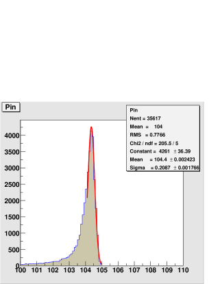
The initial momentum distribution of electrons entering the tracker and satisfying the criteria mentioned above is shown in Figure  4. This distribution is the a narrow one and can be fitted by a Gaussian with a standard deviation $\sigma$ = 0.21 MeV/c and average momentum P_in = 104.4 MeV/c in the range 104.2 MeV/c - 105 MeV/c. The width of the initial distribution of electrons is small in comparison with the total width of the momentum distribution reconstructed in the straw hit center approximation.

In Figure  5 an initial map of real and background tracker hits in all tracker’s views is shown as an example for a first simulated event. We will call it the sample event in the following. The number of real tracker hits is 29 and the number of background hits is 260 in this event. The real hits are depicted as cyan spots and the background ones are shown as red spots. Note that in the figure all 12 views were joined in one for all 18 tracker modules.

Figure 5: Plot of real + background tracker hits before the selection procedure.

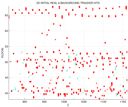
One can see from the initial distribution of tracker hits that some of background hits are concentrated along straight lines ( Figure  5) providing a typical signature of Compton electrons from photon background.

The procedure of the pattern recognition and fitting without drift time in the presence of background can be described by the following steps:

1) Rejection of hits produced by Compton electrons.

$\bullet$ A grouping containing 6 modules is taken for a given view. If in this grouping there are $N_{1}>2$ hits with the same tube number (same straw (x^′) coordinate) the corresponding hit numbers are recorded. If, in a second grouping displaced by one module from the first, there are $N_{2}>2$ hits with the same tube numbers as at the initial position of the grouping then hits from the first and the second grouping are marked as Compton electron hits. The procedure is repeated in forward and backward directions. At the end of this step all marked hits are temporary removed from the following analysis. This selection typically reduces twofold the number of background hits. Also about 5$\%$ of the real hits are rejected by the procedure but later they can be restored.

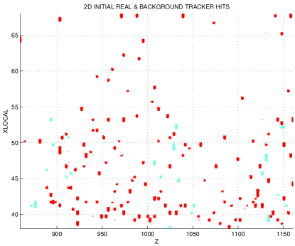
Figure  6 demonstrates the remaining tracker hits after application of the rejection procedure to the sample event. The suppression of background hits is evident.

Figure 6: Plot of real + background tracker hits after the first selection procedure.

2) Selection based on calorimeter and tracker hits.

To reconstruct the helix parameters four hits are needed. To reduce the number of four hit combinations the calorimeter hit is used in each combination. The calorimeter coordinate resolution is $\sigma=1.5$ cm which is ten times greater than tracker hit resolution in the straw hit center approximation. In spite of the poor coordinate calorimeter resolution it is possible to get a significant background suppression.

This procedure is described by the following steps:

$\bullet$ For a given view all possible three hit combinations are chosen and four hits are formed by adding a calorimeter hit to the three hit combinations. The mathematical approach described above is applied to four hits. The algorithm allows us to calculate $R$ , $\cos\theta$ , $z_{0}^{\prime}$ , $x_{0}^{\prime}$ in the chamber system of coordinates. Only the combinations that survive a cut-off in the particle momentum $p_{\min}=94MeV/c<p<p_{\max}=114MeV/c$ and pitch angle $\theta_{\min}=41.4^{\circ}<\theta<\theta_{\max}=66.4^{\circ}$ are retained for subsequent analysis.

$\bullet$ A fifth hit from a different view than the four hit combination is added. This allows us to calculate all 5 helix parameters in the global system of coordinates. A cut-off in $x_{0}$ and $y_{0}$ is applied at this step to five hits. The coordinates $x_{0},y_{0}$ are required to be in an acceptable range $-40<x_{0},y_{0}<40$ cm, where the range is determined by the GEANT simulation

$\bullet$ We look for hits correlated in 3 dimensions to choose good five hit combinations. For each selected five hit combination using the found helix parameters we reconstruct the helix, calculate all crossings of the tracker chambers for the reconstructed trajectory and define the total number of crossings N. Then we calculate how many times M at least one tracker hit matches the crossing in a road $\pm$ 3 cm. In an ideal case M should be equal to N.

$\bullet$ The probability is evaluated to get M hits in the road. The probability that M of N crossings are in the road is estimated by a trial function

$$\mathit{Prob}=\frac{N!}{M!(N-M)!}\epsilon^{M}(1-\epsilon)^{N-M}$$

where   $\epsilon$ is the probability of that there is a hit in the road within $\pm$3 cm.

If the total probability Prob is greater than the threshold probability then the given helix is considered as a good candidate. The threshold probability and  $\epsilon$ were found empirically to be 0.001 and 0.95, respectively.

As an output of the previous steps we get a collection of valid five hit combinations (helices). An individual hit is kept if it is in any valid hit combination, providing a list of good tracker hits. It is worth emphasizing that, due to the strong spatial correlations between the helix hits in comparison with the un-correlated background, the number of false hits is reduced drastically on applying the road requirement. On average the number of background hits is reduced due to this step by a factor 20.

In Figure  7 the surviving hits are shown. The significant reduction of background hits can be seen by comparing Figure  6 and Figure  7.

Figure 7: Plot of real + background tracker hits after the second selection procedure.

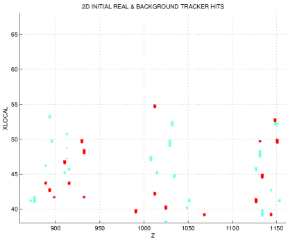
Note that at this step no real hits are removed for the sample event.

3) Selection based on tracker hits.

In this selection procedure the tracker hits found in step 2 are used. This procedure repeats the previous one with the following changes:

$\bullet$ Hits are chosen only from the tracker hits which allows to improve the performance of the selection procedure since tracker hit coordinates are defined significantly better than calorimeter hit coordinates.

A plot of the number of four hit and five hit combinations in the presence of the background (in average about 120 and 630 respectively) is shown in Figure  8 (a) and (b).

Figure 8: Number of four hit and five hit combinations.

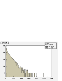
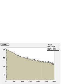
As seen in Figure  8 these distributions are broad ones reaching a few thousand combinations.

$\bullet$ For each five hit combination selected above we evaluate the position of a hit in the calorimeter $x_{eval}$ , z_eval on the basis of the defined helix parameters. The hit combination is accepted only if the evaluated hit matches the calorimeter hit within a road : $\left|x_{calo}-x_{eval}\right|<7cm$ .

$\bullet$ Parameters at this step are more restrictive: the road width is taken to be 0.75 cm and the probability to be within the road $\epsilon$ = 0.97.

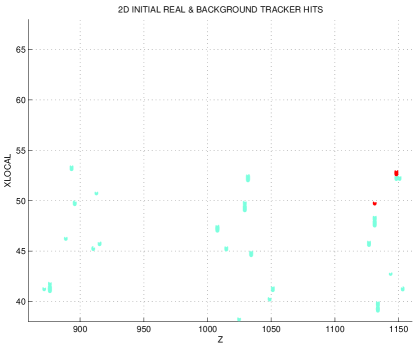
Figure  9 shows tracker hits remaining after this step for the sample event. The number of background hits is reduced typically by a factor 4 - 5 due to this step.

Figure 9: Plot of real + background tracker hits after the third selection procedure.

4) Selection including restored tracker hits.

$\bullet$ Some real tracker hits are lost at previous steps of the procedure especially at Compton electron hits rejection. To restore the lost hits an average helix for a given event is reconstructed and tracker hits that match the average helix in a road $\pm$1 straw are added to the list of valid tracker hits obtained above.

$\bullet$ Step 3 of the procedure is repeated for the extended list of tracker hits. On average the list of valid hits is extended by 1 real and 2 background hits.

$\bullet$ The union of all hits in valid five hit combinations in the extended list is used to provide an input for an average helix. A global fit is applied to reconstruct the helix parameters on the basis of the list of the selected tracker hits and the parameters of the average helix are considered as a starting point for the fit.

In this section the pattern recognition procedure without drift time based on the straw hit center approximation was developed. In this approximation no ambiguity due to mirror hits arises and the total momentum is reconstructed with the standard deviation $\sigma$ = 0.45 MeV/c. The selection procedure based on 3D space correlations between real tracker hits inside the road significantly reduces background. The overall background rejection factor is about 130 for the pattern recognition procedure without drift time.

Pattern recognition with drift time

The second stage in the pattern recognition procedure uses the fitted helix and drift time for hits selected at the first stage. The reconstruction of helix parameters can be improved by taking into account that in addition to a straw coordinate for each hit a chamber gives the radius r calculated from the measured drift time $t_{i}^{meas}$. The errors ($\sigma$) in radius measurements were taken to be 0.2 mm. This radius r carries an ambiguity as to whether the track passed left or right of the wire. The search of two possible up and down hit positions lying on the circle of radius r is based on the fitted helix obtained previously in the straw hit center approximation. We can call these up and down points as true and mirror ones. Up and down points are extracted (see Figure  10) from the intersections of a normal to the helix through the straw center and the circle of the drift radius r. In this case coordinates of up and down points are given by

$$x_{\prime}=x_{c}\mp rsin\beta;~{}~{}~{}~{}~{}z=z_{c}\pm rcos\beta;\\ ~{}~{}~{}~{}~{}tan\beta=-(R_{T}/R_{L})sin((z_{c}-z_{0}^{\prime})/R_{L})$$ (8)

Figure 10: Reconstruction of up and down points by the helix obtained in the straw hit center approximation.

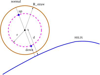
The uncertainties $\Delta s$ (see Figure  11) in the determination of up and down point positions are small and can be evaluated in the following way. The direction of 2D helix in the chamber coordinate system is given by $tan\beta$ (see Figure  11 and Eq.(8)).

Figure 11: Uncertainties in up and down point positions.

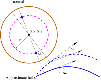
Since the uncertainty in $R_{T}$ is the dominant one the uncertainty in the direction of the helix is of the order $\Delta\beta/\beta\sim\Delta R_{T}/R_{T}\sim\Delta R/R\sim\Delta P/P$ where $\Delta P/P<0.01,\beta\sim 1$.

The uncertainty in the determination of up or down point position
$\Delta s\sim\Delta\beta$ r $<\beta(\Delta P/P)r_{tube}\sim 1\times 10^{-2}\times 0.25$ cm $\sim 25\mu$m which is much less than a measurement precision 200 $\mu$m.

To reject background hits remaining after pre-selection stage and to resolve the up - down ambiguity the deterministic annealing filter (DAF) and the Kalman filter (KF) are applied.

In principle at this stage the Kalman filter (KF) approach kalman could be applied. However an application of the Kalman filter (see Appendix A) requires that the problem of assignment of hits to a track has been entirely resolved by the preceding selection procedure. If this is not the case the filter has to run on every possible assignment choosing the best one according to the chi-square criterion. For the number of tracker hits greater than 15 this combinatorial search is computationally expensive and practically unfeasible. Therefore as the last step of pattern recognition we will use the deterministic annealing filter (DAF)  daf .

DAF is a Kalman filter with re-weighted observations (see Appendix B). For the DAF procedure we introduce artificial layers placed at the chamber straw centers in order to have competing true and mirror points in one layer. To overcome the problem of insufficient information in the initial phase of the filter, an iterative procedure is applied. After a first pass of filter and after smoothing, the track position can be predicted in every layer of the tracker. Based on these predictions, the assignment probabilities for all competing hits can be calculated in every layer. If the probability falls below a certain threshold, the hit is excluded from the following consideration. The assignment probabilities of the remaining hits are normalized to one and used as the weights in the next iterations of the filter.

In our case the operation of DAF is described by the following steps:

$\bullet$ every true and mirror point is projected on a layer corresponding to the center of straw in the direction defined by the fitted helix for a given event.

$\bullet$ initial probabilities of competing points in the layer are assumed to be equal.

$\bullet$ annealing schedule is chosen according to the following formula
$V_{n}=V(\frac{50}{f^{n}}+1)$ for a variance of observations, where V = $\sigma^{2}$ and $\sigma$ = 200 $\mu$m. The annealing factor f is chosen to be either 1.4 or 2.

$\bullet$ standard Kalman filter runs on all layers taking observations as weighted mean according to assignment probabilities.

$\bullet$ the filter runs in the opposite direction, using the same weighted mean as the forward filter. By taking a weighted mean of the predictions of both filters at every layer, a smoothed state vector and its covariance matrix are obtained.

$\bullet$ based on these predictions and the covariance matrix, the assignment probabilities of the hits are calculated. If combined hit probability for true and mirror point falls below a certain threshold ($10^{-7}$), the hit is rejected. The assignment probabilities of the remaining points in the layer are normalized to one and used as the weights in the next iterations of the filter.

$\bullet$ iterations in n stop if one of the following conditions is satisfied:
1)for the reconstructed track $\chi^{2}>\chi^{2}_{max}$ where $\chi^{2}_{max}$ = 1000 or $\chi^{2}<0$.
2)for the reconstructed initial momentum $P_{in}<94MeV/c$ or $P_{in}>114MeV/c$
3)variation of $\chi^{2}$ is small in comparison with the previous iteration $|\chi^{2}_{n+1}-\chi^{2}_{n}|/\chi^{2}_{n}<0.01$.

$\bullet$ when iterations stop (on average after 7 iterations) The DAF procedure is repeated for the different annealing factor f. From results corresponding to two annealing factors we choose that one corresponding to the minimum $\chi^{2}$.

Figure  12 shows the distribution of tracker hits for the sample event (recall that initially we had 260 background hits for this event). There are no surviving background hits and missing real hits in this case. Reconstructed lobes are clearly seen in the Figure. We conclude that DAF is effective in rejection of background hits remaining after pre-selection procedure and also it provides a good starting point for the track reconstruction.

Figure 12: Plot of real + background tracker hits after the DAF selection procedure.

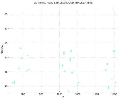
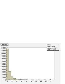
Figure  13(a) represents the number of real hits lost by the pattern recognition procedure. Some of the real tracker hits (0.8 hits $\sim 2.7\%$) are lost due to the selection procedure.

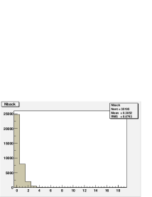
Figure  13(b) represents the number of background hits remaining after the selection procedure. As one can see from Figure  13(b) the number of background hits remaining is 0.38 hits in comparison with the primary 300 hits. So a total background suppression factor is 300/0.38 $\approx$ 800.

Figure 13: Distributions in the number of missing real hits and remaining background hits.

V Reconstruction based on Kalman filter

Background studies presented in this subsection are based on the application of the Kalman filter to hits selected by previous pattern recognition procedure.

At this stage the reconstruction is based on the hits selected by the pattern recognition procedure described above.

In principle we could use the results obtained by DAF for the track reconstruction but our analysis shows that an application of a combinatorial Kalman filter to hits selected by DAF provides better precision.

In the last decade the Kalman filter (KF) approach kalman has been extensively exploited for track fitting in high energy physics. This approach possesses the following features for effective track fitting:
$\bullet$ multiple scattering and energy losses are included in a natural way;
$\bullet$ a 3D trajectory is restored that approximates closely the real one;
$\bullet$ complex tracker geometries are handled in a simple way;
$\bullet$ N$\times$N matrix inversion, where N is the total number of measurements, is avoided;
$\bullet$ control for error propagation is provided;
$\bullet$ trajectory is reconstructed progressively from one measurement to the next, improving the precision with each step;
$\bullet$ initial and final momenta of a particle crossing the tracker are reconstructed.

The KF is very useful because it simultaneously finds and fits the track; it is much more economical than the conventional least-squares global fit. The KF is a “progressive” step by step method whose predictions are rather poor at the beginning of the track at the first stage of filtering. Since a state vector ${\bf{x}_{k}}=(x,y,t_{x},t_{y},1/p_{L})$ at point k (see definitions in Appendix A) has five parameters we need approximately $\simeq$ 6-7 straw hits to get good KF prediction precision. The prediction step, in which an estimate is made for the next measurement from the current knowledge of the state vector, is very useful to discard noise signal and hits from other tracks. Assuming the validity of the helix track model for each step, the KF propagates the track in 3D space, from one 2D surface to the next.

Below we will use the standard notations:

$\bf{x}_{k+1}^{k}$ is a prediction, i.e. the estimation of the “future” state vector at position “k+1” using all the “past” measurements up to and including “k”.

$\bf{x}_{k}^{k}$ is a filtered state vector, i.e. the estimation of the state vector at position “k” based upon all “past” and “present” measurements up to and including “k”.

The same notations will be held for the covariance matrix $\bf{C}$, noise matrix $\bf{Q}$ and so on.

The Kalman filter algorithm can be divided into three major steps.

INITIALIZATION

The KF can start from arbitrary parameters and an infinite covariance matrix but for track finding applications it is significantly better to fix somehow the initial state if possible.

The initialization of forward and backward KF algorithms is quite simple. It starts from the artificial point and initial parameters calculated from the previous stage of reconstruction procedure. The initial covariance matrix is empirically found to be diagonal with matrix elements being much greater than the corresponding uncertainties: $\bf{C}_{0}^{0}$ = (0.3,0.3,0.03,0.03,0.000003).

FILTERING

Once the KF is initialized it makes standard consequent steps. The current state at the k-th step is defined by the state vector $\bf{x}_{k}$, the state covariance matrix $\bf{C}_{k}^{k}$ and the current straw hit. To take the (k+1)-th step it is necessary to:

$\bullet$ update $\bf{x}_{k}^{k},\bf{C}_{k}^{k}$ to take into account the ionization losses
$\bullet$ define the next hit object (up or down point)
$\bullet$ propagate the parameters and the covariance matrix to: $\bf{x}_{k}^{k}\rightarrow\bf{x}_{k+1}^{k}$, $\bf{C}_{k}^{k}\rightarrow\bf{C}_{k+1}^{k}$
$\bullet$ update $\bf{C}_{k+1}^{k}$ to take into account multiple scattering $\bf{C}_{k+1}^{k}\rightarrow\bf{C}_{k+1}^{k}+\bf{Q}_{k}$
$\bullet$ calculate the Kalman matrix $\bf{K}_{k+1}$
$\bullet$ update the covariance matrix $\bf{C}_{k+1}^{k+1}$
$\bullet$ calculate residuals $\bf{r}_{k+1}^{k+1}$ and their covariance matrices $\bf{R}_{k+1}^{k+1}$
$\bullet$ calculate the incremental $\chi^{2}=(\bf{r}_{k+1}^{k+1})^{T}(\bf{R}_{k+1}^{k+1})^{-1}\bf{r}_{k+1}^{k+1}$
$\bullet$ store all information defining the new state

SMOOTHING

In the standard Kalman filter algorithm the smoothing is a well defined procedure. Smoothing allows one to obtain the best estimate of the track parameters at any trajectory point using all hit information accumulated during the KF propagation.

Figure  14 (a) displays the results of the KF forward filtering for the total momentum Ptot reconstruction at each tracker hit position. Figure  14 (b) displays how the KF smoother, based on all hit information accumulated during the KF filtering, improves the total momentum Ptot reconstruction at each tracker hit position.

Figure 14: The total momentum reconstructed by the forward Kalman filtering a) and by the smoothing b) for each hit of a selected event. The y-axis is Ptot, the x-axis is the z-ordered hit number.

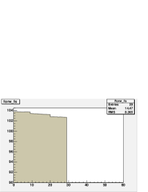
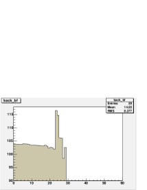
Figure  15 (a) displays the results of the KF backward filtering for the total momentum Ptot reconstruction at each tracker hit position. Figure  15 (b) displays how the KF smoother, based on all hit information accumulated during the KF filtering, improves the total momentum Ptot reconstruction at each tracker hit position.

Figure 15: The total momentum reconstructed by the backward Kalman filtering a) and by the smoothing b) for each hit of a selected event. The y-axis is Ptot, the x-axis is the z-ordered hit number.

The Kalman filter approach is effective in the resolving of up - down ambiguity. By applying the Kalman filter at each step up and down points are considered and the point providing the best $\chi^{2}$ for the trajectory is selected as the true point. This procedure is approximately linear in the number of tracker hits in comparison with the a combinatorial search, which is not feasible.

At this reconstruction stage due to left-right ambiguity for the straw drift chamber we have a set of true and mirror points for each straw hit. As discussed above the reconstruction procedure for each tracker hit defines true and mirror points and one of them is close to the real point with high precision $\simeq$ 25 $\mu$m. So we can formulate our goal as to find a true point combination for N straw hits in the presence of N mirror points.

The procedure to find the best approximation to the true point combination for N straw hits in the presence of N mirror points for one track from a muon-electron conversion event is based on the following steps:

$\bullet$ chose the first eight straw hits and built $2^{8}$ (256) possible hit combinations corresponding to up and down points. The KF forward and backward procedures described above are applied to these combinations. Only those combinations which satisfy a rather loose $\chi^{2}$ cut, $\chi^{2}<$ 30, are retained (typically about 10 out of the initial 256 combinations);

$\bullet$ make a loop for all retained combinations with fixed up and down points for the first eight straw hits. For the 9th and higher straw hit, the up and down point choices are take into account and the point with minimal incremental $\chi^{2}$ for this point is selected for the further KF propagation step. If both incremental $\chi^{2}$ satisfy the cut $\chi^{2}<$ 10 the second point is stored in the stack to make an iterative loop. A single combination of all possible steps defines a candidate track. At this stage on average 45 candidate tracks are stored in the stack per event;

$\bullet$ make a loop for all combinations from the stack. For each new hit added to the hits restored from the stack again the two up and down point choices are taken into account and the point with the minimal incremental $\chi^{2}$ for this point is selected for the further KF propagation step;

$\bullet$ select up and down track combinations with the minimal $\chi^{2}$ for the track;

$\bullet$ select a track satisfying the cut $\chi^{2}<$ 70;

$\bullet$ select a track with the difference between the forward (Pin_f) and backward (Pin_b) reconstructed input momentum satisfying the cut $|Pin\_f-Pin\_b|<$ 0.7 MeV/c.

The Kalman filter reconstructs a trajectory of a particle in three dimensions. The trajectory is bent each time it crosses a tracker plane due to multiple scattering. Therefore, the reconstructed track is a set of helices that intersect at the planes. This is the track followed by the particle.

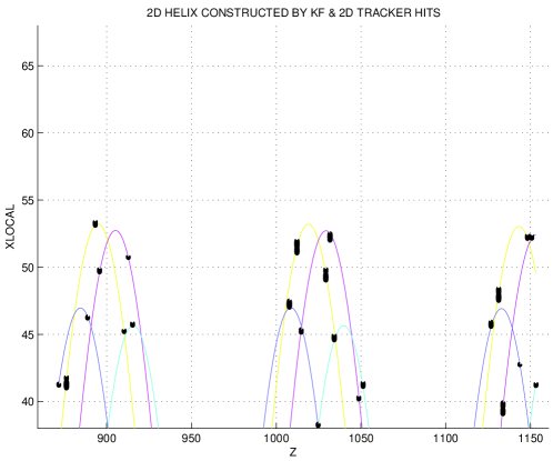
Figure  16 displays a 2D projection of 3D trajectory reconstructed by the Kalman filter for the sample event. As above in this figure all 12 views were joined in one for all 18 tracker modules. The 2D trajectory is shown only for sensitive area of the tracker and for each view the trajectory is in a different color. For the sample event real hits are in four tracker’s views and the reconstructed lobes for these views are clearly seen in the figure.

Due to a scale in this figure the 2D trajectory looks as an ideal sine curve and tracker hits look like spots of different size. In order to see a detailed behavior of the trajectory and hit positions a dynamical zoom is applied to a rectangular region indicated in Figure  16 in the x-range 49-50 cm and z-range 1029-1029.5 cm.

Figure  17 demonstrates the magnified region of the tracker. Blue line in the figure represents the reconstructed trajectory. Two circles represent two hits in chamber. These circles look like ellipses due to different axis scales.

Figure 16: Plot of real + background tracker hits after the DAF selection procedure.

Figure 17: Zoom enlargement of the region in Figure  16.

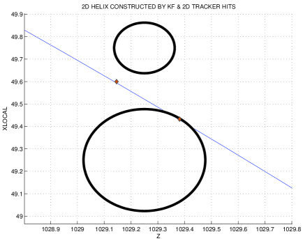
Radii of the circles are directly proportional to the drift times. For illustrative purposes two nearest to the straw center points corresponding to the real trajectory obtained in Monte Carlo simulation are shown in the Figure in the form of diamonds   (note that in the pattern recognition procedure only radii were used but not these points). The measurement uncertainty was taken into account assuming that circle radii are distributed normally about the simulated radii with $\sigma=200\mu$m. For this reason the position of one of the nearest points is not on a circle in Figure  17.

In Figure  17 due to the corresponding scale the trajectory looks like a straight line. It is tangent to one of two circles obtained on the basis of drift time. In the region under consideration the deviation of the trajectory from the nearest point is less than 0.2 mm. The change in the direction of the trajectory due to multiple scattering can not be seen in the Figure because of the smallness of the average angle of the scattering.

Figure  18 shows transverse xy-projection of the trajectory for the sample event. In this projection the trajectory looks approximately as a circle.

Figure 18: The transverse projection of the 3D trajectory reconstructed for the sample event.

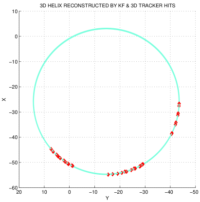
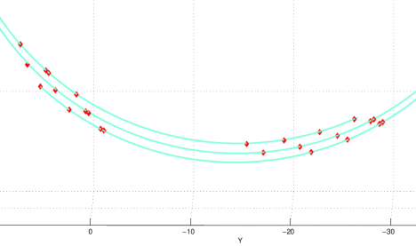
However if a specific region of the tracker is magnified by the dynamical zoom one can see in Figure  19 that the shape of the circle is distorted due to multiple scattering and energy loss. More than two turns of trajectory are clearly seen in the Figure.

Figure 19: Zoom enlargement of the region in Figure  18.

Note that by using the KF filter a momentum of a particle can be reconstructed at any point of the tracker. For our purposes the most important is the momentum of a particle entering the tracker, which in the following we will call the input momentum.

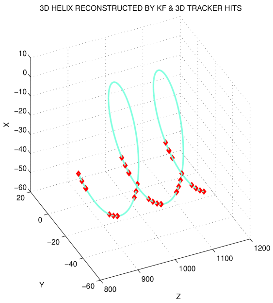
Figure  20 demonstrate 3D trajectory reconstructed for the sample event. The trajectory looks in this scale as a helix, but we remind that it consists of many helix parts. Also in the Figure tracker’s hits generated by Monte Carlo simulation program are shown.

Figure 20: 3D trajectory reconstructed for the sample event.

The distribution in the difference between the initial momentum (Pin_f) reconstructed by the Kalman filter and the generated initial momentum (Pin) is shown in Figure  21 in linear (a) and logarithmic (b) scale. According to this distribution the intrinsic tracker resolution is $\sigma$ = 0.12 MeV/c if one fits the distribution by a Gaussian in the range -0.3 - 0.7 MeV/c.

Figure 21: Distribution in the difference between the input reconstructed momentum based on the Kalman filter and the simulated input momentum with background.

Figure 22: Distribution in the input momentum reconstructed by the Kalman filter with background.

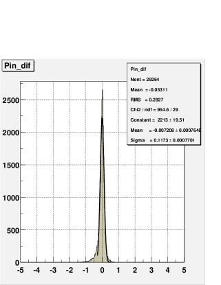
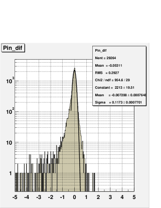
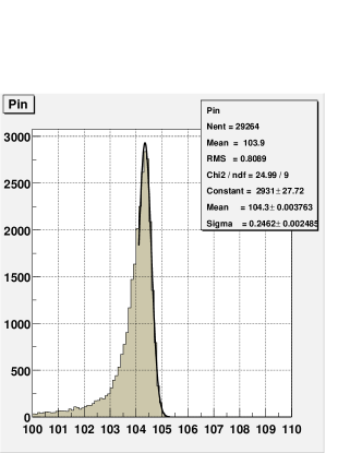
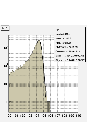
Figure  22 shows a distribution in the input momentum (Pin_f) reconstructed by the Kalman filter in linear (a) and logarithmic (b) scale with background. This distribution is characterized by the standard deviation $\sigma$ = 0.25 MeV/c of the reconstructed input momentum for a Gaussian fit in the range 104-106 MeV/c.

Note that the trajectory reconstructed by the Kalman filter consists of many helix parts. The reconstructed input momentum resolution by the Kalman filter is $\sigma$ = 0.25 MeV/c. This resolution significantly better than the resolution $\sigma=0.35$ MeV/c obtained by a single helix fit.

The overall reconstruction acceptance is 22.1 $\%$ for muon conversion events with the momentum above a threshold momentum of 103.6 MeV/c.

Comparing these results with the results of the reconstruction without background we get the difference in tracker resolution 1.5 % and the difference 2.7 % in overall acceptance (see Appendix C). Therefore the tracker resolution and overall acceptance are not affected significantly at the considered background level (explained in Section 3).

A summary of the critical selection criteria used in the momentum reconstruction is shown in Table  2. The efficiencies are for the selection criteria applied in consecutive order.

An overall acceptance for muon conversion events with momentum above threshold momentum $P_{th}$ is 22.1% . We define a threshold momentum, above which events are considered as the useful ones by $P_{th}=P_{max}-\Delta$, where $P_{max}$ = 104.3 MeV/c the most probable reconstructed momentum. If $\Delta$ = 0.7 MeV/c is chosen then $P_{th}$ = 103.6 MeV/c.

Table 2: A summary of the reconstruction selection criteria

Selection criterion	Efficiency
Calorimeter energy above 80 MeV	0.53
Required pitch angle at the tracker	0.86
At least 15 hits in the tracker	0.87
Position match in the calorimeter	0.95
Requirements on fit quality	0.79
Detected energy above 103.6 MeV	0.74
Overall acceptance	0.22

The main factors entering into the experimental sensitivity are the running time, the proton intensity, the probability per proton that a $\mu$ is produced, transported and stopped in the stopping target, the fraction of stopped muons that are captured (as opposed to decay), the trigger efficiency and the tracker reconstruction acceptance. We do not include in this table loss of events due to accidental cosmic ray vetoes, dead-time losses and losses due to straw chamber inefficiencies, all of which are expected to be small. According to our analysis taking into account the straw efficiency 97% the overall acceptance is reduced from 22.1% to 21.7% .

Table  3 shows expected MECO sensitivity for a one year ($10^{7}$ s) run.

Table 3: A summary of the expected MECO sensitivity.

Running time (s)	$10^{7}$
Proton flux (Hz)	$4\cdot 10^{13}$
Probability of $\mu$/p transported and stopped in target	0.0025
$\mu$ capture probability	0.6
Fraction of $\mu$ which are captured in time window	0.49
Trigger efficiency and the selection criteria	0.22
Detected events for $R_{\mu e}=10^{-16}$	6.5

Muon DIO events are the most important background for the experiment. The main background from muon DIO events in the presence of background tracker hits was simulated and reconstructed. Based on the simulated DIO events in the momentum range above 100 MeV/c the track pattern recognition and momentum reconstruction were performed in the presence of background tracker hits (protons, neutrons, photons, DIO) by applying the selection criteria discussed above.

Figure 23: Distributions of DIO reconstructed momentum in the presence of the background above 100 MeV/c .

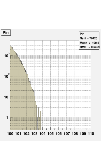
The number of primary DIO events simulated in the momentum range above 100 MeV/c was 10 times more than expected and 3 background events were found (see Figure  23). So the background is expected to be 0.3 events.

It is important to note that input reconstructed momenta for these three background events are very close to simulated input momenta. The input simulated momenta 103.48, 103.6 and 103.74 MeV/c for these events have to be compared with input reconstructed momenta 103.6, 103.76 and 103.8 MeV/c, respectively.

At the present level of pattern recognition and momentum reconstruction studies we can expect the background from DIO events in the range above 100 MeV/c $\sim$0.3 events compared to 6.5 signal events for $R_{\mu e}=10^{-16}$.

VI Conclusion

A study of the impact of background on the performance of the transverse tracker proposed for the MECO experiment is presented. Background from capture protons, neutrons and photons, and from muon decay in orbit was generated using GEANT3. The effective average straw tube rate from these sources was 800 kHz at the proposed muon beam intensity of $2\times 10^{11}\mu^{-}/sec$.

A pattern recognition procedure based on a Kalman filter technique was developed to suppress background and assign hits to tracks. In the first stage of this procedure, straw hit center coordinates, without drift time information, were used to reduce the background by a factor $\sim$ 130. In the second stage, the full drift time information and a deterministic annealing filter were used to obtain an additional six-fold suppression. The total suppression of 800 reduces the number of background hits on average from an initial value of 300 to approximately 0.4 per event. About 0.8 hits of the 29 real hits typically recorded, or 2.7 $\%$, are lost in the process.

It was found that in the presence of background the resolution of the tracker is $\sigma=0.12$ MeV/c and the overall setup acceptance for muon conversion events with momentum above the threshold momentum 103.6 MeV/c is about 22 $\%$. At the considered background level the tracker resolution and the overall acceptance are not affected significantly by presence of the background: the tracker resolution is changed by 1.5 % and the overall acceptance by 2.7 %.

Additional constraints on the background, not considered here, may be imposed if the drift time measurement is supplemented by a measurement of the pulse amplitude at the anode wire. A straightforward, crude measurement of the amplitude is sufficient to reduce significantly the background from heavily ionizing particles, i.e., the capture protons that comprise 30 % of the background hits in the above study. We estimate too that a significant background suppression, of 10-20, would be achieved if resistive anode wires were used in place of conducting wires to obtain a measurement of the hit position along the wire. This would improve the resolution as well.

At the present level of pattern recognition and momentum reconstruction studies the background from DIO events above 100 MeV/c is about 0.3 events. This is to be compared to 6.5 signal events for $R_{\mu e}=10^{-16}$.

The study carried out shows that the developed procedures of pattern recognition and momentum reconstruction in the case of the transverse tracker provide a required precision for lepton number violation search at a sensitivity level about $10^{-17}$.

We wish to thank A. Mincer, P.Nemethy, J.Sculli and one of us (R.K.) thanks W.Willis for fruitful discussions and helpful remarks.

APPENDIX A. KALMAN FILTER AND ITS APPLICATION TO TRACK FITTING

The Kalman filter is an algorithm that processes measurements to deduce an optimum estimate of the past, present, or future state of  a dynamic system by using a time sequence of measurements of the system behavior, plus a statistical model that characterizes the system and measurements errors, plus initial condition information.

The Kalman filter addresses the general problem of trying to estimate at different points ($1\leq k\leq n$) the state $\bf{x}_{k}$ of a discrete process that is governed by the linear stochastic difference equation

$$\bf{x}_{k}=\bf{F}_{k-1}\bf{x}_{k-1}+\bf{w}_{k-1}$$ (9)

with a measurement $\bf{m}_{k}$ that is

$$\bf{m}_{k}=\bf{H}\bf{x}_{k}+\bf{\varepsilon}_{k}.$$ (10)

The system equation (9) is not deterministic since the track experiences stochastic processes such as multiple scattering, bremsstrahlung, etc. These processes are taken into account by the process noise $\bf{w}_{k}$ . $\bf{\varepsilon}_{k}$ represents the measurement noise. $\bf{w}_{k}$ and $\bf{\varepsilon}_{k}$ are assumed to be independent of each other with zero expectation values:

$E\{\bf{w}_{k}\}=0,\qquad cov\{\bf{w}_{k}\}=\bf{Q}_{k}$ ,   $1\leq k\leq n,$

$E\{\bf{\varepsilon}_{k}\}=0,\qquad cov\{\bf{\varepsilon}_{k}\}=\bf{V}_{k}$ ,   $1\leq k\leq n,$

where $\bf{Q}_{k}$ and $\bf{V}_{k}$ are process noise and measurement noise covariances, respectively.

Eq.(9) in the absence of the last term is the standard equation of motion with a propagator $\bf{F}_{k-1}$ (transport matrix). Note that at the moment $\bf{F}_{k-1}$ is assumed to be constant.

Regarding a track in space as a dynamic system the filtering technique is applied to the track fitting. For example, in the case of a particle moving in magnetic field this can be done naturally by identifying the state vector $\bf{x}_{k}$ of the dynamic system with a vector $\bf{x}_{k}=(x,y,\tan\theta_{x},\tan\theta_{y},1/p_{L})$ of 5 parameters uniquely describing the track at each point of the trajectory. The $\bf{F}$ matrix propagates the state vector on one plane to the state vector on the next plane combining position information with directional information. The transport matrix implicitly contains information about a gap between planes.

In general the set of parameters $\bf{x}_{k}$ is not measured directly; only a function of $\bf{x}_{k}$ , $\bf{H}\bf{x}_{k}$ is observed. For example, in the case of the transverse tracker one does not measure $\bf{x}_{k}$ but $x\prime=x\cos\alpha+y\sin\alpha$ in the chamber coordinate system which corresponds to

$$\bf{H}=(\cos\alpha,\sin\alpha,0,0,0)$$ (11)

There are three types of operations to be performed in the analysis of a track.

• Prediction is the estimation of the “future” state vector at position “k” using all the “past” measurements up to and including “k-1”. $\bf{x}_{k}^{k-1}$ is a prediction (a priori state estimation).

• Filtering is the estimation of the state vector at position “k” based upon all “past” and “present” measurements up to and including “k”. $\bf{x}_{k}^{k}$ is a filtered state vector (a posteriori state estimation).

• Smoothing is the estimation of the “past” state vector at position “k” based on all “n” measurements taken up to the present time. $\bf{x}_{k}^{n}$ is a smoothed state vector.

The first step to estimate $\bf{x}_{k}$ is the prediction (time update):

$$\bf{x}_{k}^{k-1}=\bf{F}_{k-1}\bf{x}_{k-1}^{k-1}$$ (12)

$$\bf{C}_{k}^{k-1}=\bf{F}_{k-1}\bf{C}_{k-1}^{k-1}\bf{F}_{k-1}^{T}+\bf{Q}_{k-1}$$ (13)

where Eq.(12) projects the state ahead and Eq.(13) projects the error covariance ahead.

The filtered estimate (measurement update) $\bf{x}_{k}^{k}$ is calculated as a weighted mean of the prediction and the observation:

$$\bf{K}_{k}=\bf{C}_{k}^{k-1}\bf{H}_{k}^{T}[\bf{H}_{k}\bf{C}_{k}^{k-1}\bf{H}_{k}^{T}+\bf{V}_{k}]^{-1}$$ (14)

$$\bf{x}_{k}^{k}=\bf{x}_{k}^{k-1}+\bf{K}_{k}[\bf{m}_{k}-\bf{H}_{k}\bf{x}_{k}^{k-1}]$$ (15)

$$\bf{C}_{k}^{k}=[\bf{I}-\bf{K}_{k}\bf{H}_{k}]\bf{C}_{k}^{k-1}.$$ (16)

Eq.(14) computes the Kalman gain matrix defining the correction to the predicted state due to the current observation. Eq.(15) updates the prediction with the measurement and Eq.(16) updates the error covariance. The error covariance may be also expressed in a computationally superior form

$$\bf{C}_{k}^{k}=[\bf{I}-\bf{K}_{k}\bf{H}_{k}]\bf{C}_{k}^{k-1}[\bf{I}-\bf{K}_{k}\bf{H}_{k}]^{T}+\bf{K}_{k}\bf{V}_{k}\bf{K}_{k}^{T}.$$ (17)

The filtering is a recursive operation. The prediction step and the filtering step are repeated for the next plane proceeding progressively from plane “1” to plane “n”. The state vector at the last filtered point contains always the full information from all points.

At each step one can calculate the filtered residuals $\bf{r}_{k}^{k}$ , the covariance matrix of the filtered residuals $\bf{R}_{k}^{k}$ and the filtered $\chi^{2}$:

$$\bf{r}_{k}^{k}=\bf{m}_{k}-\bf{H}_{k}\bf{x}_{k}^{k}$$

$$\bf{R}_{k}^{k}=\bf{V}_{k}-\bf{H}_{k}\bf{C}_{k}^{k}\bf{H}_{k}^{T}$$

$$\chi_{k}^{2}=\bf{r}_{k}^{kT}(\bf{R}_{k}^{k})^{-1}\bf{r}_{k}^{k}$$

where $\chi_{k}^{2}$ is $\chi^{2}$ - distributed with dim($\bf{m}_{k}$) degrees of freedom. The total $\chi^{2}$ of the track is given by the sum of the $\chi_{k}^{2}$ contributions for each plane.

The system of equations defining the Kalman filter represents an asymptotically stable system, and therefore, the estimate of the state vector $\bf{x}_{k}^{k}$ becomes independent on the starting point $\bf{x}_{0}^{0}$ , $\bf{C}_{0}^{0}$ as k is increased.

When the last plane (nth) is taken into account the Kalman filter performs the final step which is a smoothing. The filter runs backward in time updating all filtered state vectors on the basis of information from all n planes. The equations describing the smoothing are given by

$$\bf{A}_{k}=\bf{C}_{k}^{k}\bf{F}_{k}^{T}(\bf{C}_{k+1}^{k})^{-1}$$

$$\bf{x}_{k}^{n}=\bf{x}_{k}^{k}+\bf{A}_{k}(\bf{x}_{k+1}^{n}-\bf{x}_{k+1}^{k})$$

$$\bf{C}_{k}^{n}=\bf{C}_{k}^{k}+\bf{A}_{k}(\bf{C}_{k+1}^{n}-\bf{C}_{k+1}^{k})\bf{A}_{k}^{T}$$

$$\bf{r}_{k}^{n}=\bf{m}_{k}-\bf{H}_{k}\bf{x}_{k}^{n}$$

$$\bf{R}_{k}^{n}=\bf{V}_{k}-\bf{H}_{k}\bf{C}_{k}^{n}\bf{H}_{k}^{T}$$

Until now it was assumed that the problem of estimation of a discrete-time process is described by a linear stochastic differential equation. However for example in the presence of a magnetic field the track propagator $\bf{F}$ is non-linear. Let’s assume that the process of a particle propagation is governed by the non-linear stochastic differential equation

$$x_{k}=f(x_{k-1})+w_{k-1}$$ (18)

with a measurement m in the form Eq.(10). f is a non-linear function. The Kalman filter can be applied to this system by linearizing the system for example about the estimated trajectory. If deviations between the estimated trajectory and the actual trajectory remain sufficiently small the linear approximation is valid. The non-linear equation (18) can be written down in the linearized form as

$$\bf{x}_{k}=\bf{f}(\bf{x}_{k-1}^{k-1})+\bf{F}\cdot(\bf{x}_{k-1}-\bf{x}_{k-1}^{k-1})+\bf{w}_{k-1}$$ (19)

where as before $\bf{x}_{k}$,$\bf{m}_{k}$ are the actual state and measurement vectors, $\bf{x}_{k}^{k}$ is a filtered estimate of the state at step k. $\bf{F}$ is Jacobian matrix

$$\bf{F}_{ij}=\partial\bf{f}_{i}(\bf{x}_{k-1}^{k-1})/\partial x_{j}$$ (20)

Therefore the complete set of extended Kalman filter equations is given by Eqs.(13)-(16),(19) by using F in the form (20).

In order to apply the extended Kalman filter to a track fitting for a particle moving in uniform magnetic field (the magnetic field is in z direction) one has to choose the state vector parameters, define the initial state vector and calculate the transport matrix $\bf{F}$, the projection matrix $\bf{H}$, and the noise matrix $\bf{Q}$. As it was mentioned above in this case the state vector can be chosen in the form ${\bf{x}_{k}}=(x,y,t_{x},t_{y},1/p_{L})$ where x, y are the track coordinates in the tracker system, $t_{x}=p_{x}/p_{L}$, $t_{y}=p_{y}/p_{L}$ define the track direction. The projection matrix H is given by Eq.(11). Due to multiple scattering the absolute value of electron momentum remains unaffected, while the direction is changed. This deflection can be described using two orthogonal scattering angles, which are also orthogonal to the particle momentum  mank . In terms of these variables the noise matrix is given by

$$\bf{Q}_{k}=<\Theta^{2}>(t_{x}^{2}+t_{y}^{2}+1)\left.\left(\begin{array}[]{ccccc}0&0&0&0&0\\ 0&0&0&0&0\\ 0&0&t_{x}^{2}+1&t_{x}t_{y}&t_{x}/p_{L}\\ 0&0&t_{x}t_{y}&t_{y}^{2}+1&t_{y}/p_{L}\\ 0&0&t_{x}/p_{L}&t_{y}/p_{L}&\frac{(t_{x}^{2}+t_{y}^{2})}{p_{L}^{2}(t_{x}^{2}+t_{y}^{2}+1)}\end{array}\right.\right)$$

For the variance of the multiple scattering angle the well-known expression is used

$$<\Theta^{2}>=(13.6MeV/p)^{2}[1+0.038\ln(t/X_{R})]t/X_{R}$$ (21)

where $X_{R}$ is a radiation length, t is a distance traveled by the particle inside a scatterer. Energy losses are taken into account by

$$p\prime=p-<dE/dx>t.$$ (22)

APPENDIX B. DETERMINISTIC ANNEALING FILTER

Track reconstruction in modern high energy physics experiments faces a significant amount of noise hits in a detector. The track fit thus is confronted with several competing hits in detector’s layers. The Kalman filter (see Appendix A) is now widely used for the reconstruction of the track parameters in high energy physics. However the application of the Kalman filter requires that the problem of assignment of the detector hits to track candidates has been entirely resolved by the preceding selection procedure. If this is not the case, the filter has to run on every possible assignment to select the best one by chi-square criterion. Obviously this approach is computationally expensive and practically unfeasible for a considerable amount of noise hits. For this reason the Deterministic Annealing Filter (DAF) was developed  daf . In DAF there is an additional validation feature eliminating hits which are not compatible with the predicted track position.

The deterministic annealing filter itself is a Kalman filter with re-weighted observations. The propagation part of DAF is identical to the standard Kalman filter.

The filtered estimate (measurement update) $\bf{x}_{k}^{k}$ at layer k is calculated as a weighted mean of the prediction $\bf{x}_{k}^{k-1}$ and the observations $\bf m_{k}^{i},i=1,2,...n_{k}$:

$$\bf x_{k}^{k}=\bf x_{k}^{k-1}+\bf K_{k}\sum_{i=1}^{{n}_{k}}p_{k}^{i}[\bf{m}_{k}^{i}-\bf{H}_{k}\bf{x}_{k}^{k-1}]$$ (23)

where ${\bf p_{k}^{i}}$ is the assignment probability of observation $\bf m_{k}^{i}$. $\bf{K}_{k}$ is the Kalman gain matrix which is given by

$$\bf{K}_{k}=[[\bf{C}_{k}^{k-1}]^{-1}+p_{k}\bf{H}_{k}^{T}\bf{V}_{k}^{-1}\bf{H}_{k}]^{-1}\bf{H}_{k}^{T}\bf{V}_{k}^{-1}$$ (24)

where ${\bf p_{k}}$ is the sum over all weights ${\bf p_{k}^{i}}$, $\bf{H}_{k}$ is the measurement matrix, $\bf{V}_{k}$ is the variance of the observations.

The covariance matrix $\bf{C}_{k}^{k}$ of the updated estimate $\bf{x}_{k}^{k}$ is written as

$$\bf{C}_{k}^{k}=[[\bf{C}_{k}^{k-1}]^{-1}+p_{k}\bf{H}_{k}^{T}\bf{V}_{k}^{-1}\bf{H}_{k}]^{-1}.$$ (25)

After completion of the forward filter a backward filter runs in opposite direction, using the same weights as the forward filter. By taking a weighted mean of the filtered states of both filters at every layer a prediction for the state vector $\bf x_{k}^{n*}$ along with its covariance matrix $\bf{C}_{k}^{n*}$ is obtained, using all hits except the ones at layer k. (The asterisk indicates that the information from layer k is not used in this prediction.) Initially all assignment probabilities for the hits in each layer are set to be equal but based on the estimated state vector $\bf x_{k}^{n*}$ and its covariance matrix, the assignment probabilities of all competing hits are then recalculated in the following way:

$${\bf{p}_{k}^{i}}\sim\varphi(\bf{m}_{k}^{i};\bf{H}_{k}\bf x_{k}^{n*},\bf{V}_{k}+\bf{H}_{k}\bf{C}_{k}^{n*}\bf{H}_{k}^{T})$$ (26)

where $\varphi(\bf x;{\bf\mu},\bf V$) is a multivariate Gaussian probability density with mean vector ${\bf\mu}$ and covariance matrix $\bf V$.

If the probability falls below a certain threshold, the hit is considered as the false one and is excluded from the list of the hits assigned to the track.

However at this step we cannot be sure in calculated probabilities especially in the initial phase due to insufficient information for the filter. This problem is overcome by adopting a simulated annealing iterative procedure. This is an additional feature of DAF.

The simulated annealing optimization algorithm is based on an analogy between the behavior of a material heated past its melting point that is slowly cooled (annealed) to form a single crystal. If the cooling proceeds slowly enough, the crystalline state reached at zero temperature will have all the atoms fixed in a perfect lattice structure, corresponding to the lowest possible energy of the system (global minimum).

In the same way in track fitting the simulated annealing allows to avoid a local minimum and find the global one corresponding to the minimum chi-square for the track.

DAF annealing algorithm can be described in the following way. The annealing schedule is chosen for example in the form ${\bf V_{N}}={\bf V}(A/f^{N}+1)$ where the annealing factor $f>1$ and factor $A>>1$. This provides that the initial variance is well above the nominal value ${\bf V}$ of the observation error but the final one tends to ${\bf V}$. After each iteration the assignment probabilities exceeding the threshold are normalized to 1 and used again as weights in the next iteration, and so on. The iterations generally are stopped if the relative change in chi-square is less than correspondent control parameter (typically of the order 0.01).

Since we deal with the stochastic process the best result can be reached repeating the DAF procedure for a few different annealing factors f and then choosing the result corresponding to the minimum chi-square.

APPENDIX C. Tracker Resolution

This appendix demonstrates the results of application of the pattern recognition and reconstruction procedure for the conversion events without background.

The distribution in the difference between the input reconstructed momentum (Pin_f) based on the Kalman filter and the simulated input momentum (Pin) is shown in Figure  24 in linear (a) and logarithmic (b) scale. According to this distribution the intrinsic tracker resolution is $\sigma$ = 0.12 MeV if one fits the distribution by a Gaussian in the range -0.3 - 0.7 MeV.

Figure 24: Distribution in the difference between the input reconstructed momentum based on the Kalman filter and the simulated input momentum without background.

Figure 25: Distribution in the input momentum reconstructed by the Kalman filter without background.

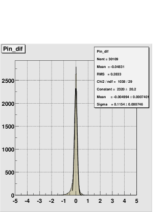
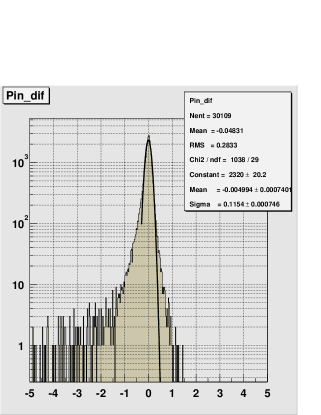
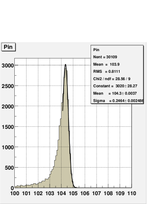
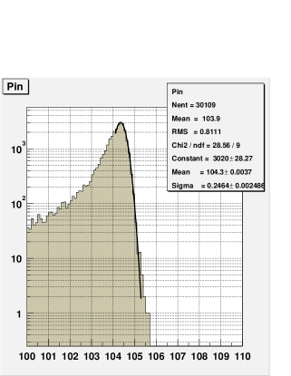
Figure  25 shows a distribution in the input momentum (Pin_f) reconstructed by the Kalman filter in linear (a) and logarithmic (b) scale without background. This distribution is characterized by the standard deviation $\sigma$ = 0.25 MeV of the reconstructed input momentum for a Gaussian fit in the range 104-106 MeV. The overall reconstruction acceptance is 22.7 $\%$ for muon conversion events with the momentum above a threshold momentum of 103.6 MeV/c.

Comparing these results with the results of the reconstruction in the presence of the background we get the difference in tracker resolution 1.5 % and the difference 2.7 % in overall acceptance. Therefore the tracker resolution and overall acceptance are not affected significantly at the considered background level.

References

- (1) J.D.Vergados, Phys.Rep. 133, 1, (1986); Y.Kuno and Y.Okada, Rev.Mod.Phys.73, 151 ,(2001).
- (2) P.Wintz, Proc. of the 1st Int.Symp. on Lepton and Baryon Number Violation, 1998, ed. by H.V.Klapdor-Kleingrothaus and I.V.Krivosheina (Inst. of Physics Publishing, Bristol and Philadelphia), 534.
- (3) A. van der Schaaf, J.Phys.G: Nucl.Part.Phys. 29, 1503, (2003).
- (4) R.M.Djilkibaev and V.M.Lobashev, Sov.J.Nucl.Phys. 49, 384, (1989).
- (5) V.Abadjev et al, MELC proposal, INR preprint 786/92, (1992).
- (6) M.Bachman et al, a research proposal to BNL AGS, (1997); NSF RSVP proposal (MECO), (1999).
- (7) S.Machida et al, a letter of intent to the J-PARC 50-GeV Proton Synchrotron Experiment, The PRIME Working Group, (2003).
- (8) R. Frühwirth and A. Stradlie, Comp.Phys.Comm. 120, 197, (1999).
- (9) R.E.Kalman, Transactions of the ASME: J.Basic Engineering, D82, 35, (1960).
- (10) P.Billoir, Nucl.Instr.Meth. 225, 352, (1984); R.Frühwirth, ibid. A262, 444, (1987); P.Billoir and S.Qian, ibid. A294, 219, (1990); E.J.Wolin and L.L.Ho, ibid. A329, 493, (1993).
- (11) R.Mankel, Hera B note (1997).