Recent Results from KamLAND

Abstract

The Kamioka Liquid-scintillator Anti-Neutrino Detector (KamLAND) has detected for the first time the disappearance of electron antineutrinos from a terrestrial source at the 99.95% C.L.[1] Interpreted in terms of neutrino oscillations $\bar{\nu}_{e}\leftrightarrow\bar{\nu}_{x}$, the best fit to the KamLAND data gives a mixing angle $\sin^{2}2\theta=1.0$ and a mass-squared difference $\Delta m^{2}=6.9\times 10^{-5}$ eV², in excellent agreement with the Large Mixing Angle (LMA) solution to the ”solar neutrino problem”.[2] Assuming CPT invariance, this result excludes other solutions to the solar neutrino problem at $>$ 99.95% C.L.

1 Reactor Antineutrino Experiments and Neutrino Oscillation

Nuclear reactors emit a calculable flux of electron antineutrinos ($\bar{\nu}_{e}$s) in all directions. For standard particle propagation, one expects a detector located a distance $L$ from the reactor to measure a flux that decreases as $1/L^{2}$. But if $\bar{\nu}_{e}$s are massive, they may ”oscillate” into undetectable flavors on the way to the detector, leading to an apparent ”disappearance” of the $\bar{\nu}_{e}$s.

Neutrinos are produced and detected in weak interactions, which couple to the weak eigenstates $\nu_{l}$, where $l=e,\mu,\tau$. For massive neutrinos, the weak eigenstates may be expressed as a linear combination of three mass eigenstates $\nu_{i}$, $i=1,2,3$, with mass $m_{i}$:

$$\nu_{l}=\sum_{i}U_{li}\nu_{i}.$$ (1)

$U_{li}$ is a $3\times 3$ unitary ”mixing” matrix and is analogous to the CKM matrix in the quark sector. As a neutrino propagates through vacuum with momentum $p_{\nu}$, the phase of each mass eigenstate will change at different rates according to

$$\nu_{l}(t)=\sum_{i}U_{li}e^{-iE_{i}t}\nu_{i},$$ (2)

where $E_{i}\approx p_{\nu}+\frac{m_{i}^{2}}{2p_{\nu}}$. At times $t>0$ the neutrino will be in a superposition of the weak eigenstates. The probability of detecting flavor $\nu_{l^{\prime}}$ at a distance $L\approx t$ from the source is then

$$P(\nu_{l}\rightarrow\nu_{l^{\prime}})=Re\sum_{i,j}U_{li}U_{il^{\prime}}^{\dagger}U_{lj}U_{jl^{\prime}}^{\dagger}e^{i\frac{m_{i}^{2}-m_{j}^{2}}{2p_{\nu}}L}.$$ (3)

In neutrino oscillation experiments, it is common to simplify to two neutrino flavors, say $\nu_{e}$ and $\nu_{\mu}$, in which case $U_{li}$ is parameterized by a single mixing angle $\theta$. In this picture, the probability of a neutrino emitted as $\nu_{e}$ to be detected as $\nu_{e}$ is then

$$P\left(\nu_{e}\rightarrow\nu_{e}\right)=1-\sin^{2}2\theta\sin^{2}\left(\frac{\pi L}{L_{osc}}\right)$$ (4)

where $L_{osc}=\frac{4\pi p_{\nu}}{\Delta m^{2}}$. Here, $\Delta m^{2}=\left|m_{1}^{2}-m_{2}^{2}\right|$ is taken to be the mass-squared difference between two ”effective” mass eigenstates relevant to $\nu_{e}\leftrightarrow\nu_{\mu}$ mixing. Note that $P\left(\nu_{e}\rightarrow\nu_{e}\right)$ is a sinusoidal function of L, hence the name ”neutrino oscillation”.

The situation becomes slightly more complicated for neutrinos propagating through matter. As first recognized by Wolfenstein[3], Mikheyev, and Smirnov[4], while all three weak states participate in neutral-current interactions with normal matter, only electron neutrinos have additional charge-current interactions with electrons in the material being traversed. This results in an effective index-of-refraction for $\nu_{e}$ different from that for $\nu_{\mu,\tau}$ by

$$\Delta n=\frac{2\pi N_{e}}{p_{\nu}^{2}}f(0),$$ (5)

where $N_{e}$ is the number-density of electrons in the material, and $f(0)$ is the forward scattering amplitude. $\Delta n$ changes the phase of the $\nu_{e}$-component relative to the other components by $2\pi$ over a distance $L_{0}$ given by

$$L_{0}=\frac{2\pi}{\sqrt{2}G_{F}N_{e}},$$ (6)

where $G_{F}$ is the Fermi constant. This phenomenon, called the MSW effect, alters the two flavor oscillation probability as follows:

$$P\left(\nu_{e}\rightarrow\nu_{e}\right)=1-\sin^{2}\left(2\theta_{m}\right)\sin^{2}\left(\frac{\pi L}{L_{m}}\right)$$ (7)

$$\tan 2\theta_{m}\equiv\tan 2\theta\left(1+\frac{L_{osc}}{L_{0}}\sec 2\theta\right)$$ (8)

$$L_{m}\equiv L_{osc}\left[1+\left(\frac{L_{osc}}{L_{0}}\right)^{2}+\frac{2L_{osc}}{L_{0}}\cos 2\theta\right]^{-\frac{1}{2}}$$ (9)

For neutrinos created in and propagating out of the sun, $L_{0}\approx 200$ km $\ll R_{sun}$, and matter effects are significant. The result is that $\nu_{e}$ disappearance experiments that use the sun as a source, such as Homestake[5], GALLEX[6], SAGE[7], Kamiokande[8], Super-Kamiokande[9], and SNO[10], individually allow values of $\tan^{2}\theta$ and $\Delta m^{2}$ over many orders of magnitude. The overlap of allowed regions from multiple experiments with different thresholds leaves a few small patches, with values around $\tan^{2}\theta\approx 1$ and $\Delta m^{2}\approx 10^{-4}$ eV² highly favored. This region is called the ”Large Mixing Angle” (LMA) MSW solution. Prior to KamLAND, another patch at lower $\Delta m^{2}\approx 10^{-7}$ eV², known as the ”LOW” MSW solution, survived at the 99.73% C.L.[10]

For neutrino experiments with artificial sources on the earth, matter effects are typically much less significant. This is because for matter with density similar to rock $L_{0}\approx 10^{4}$ km, larger than the radius of the earth. Thus for these sources the modifications to the oscillation parameters can be viewed as perturbations on the vacuum parameters, and for short enough oscillation lengths can be neglected.

Artificial $\nu$ sources for oscillation experiments typically take one of two forms: neutrino beams or nuclear reactors. These two sources comprise a highly complementary experimental program in neutrino oscillation. Neutrino beams in general require very long baselines for good $\Delta m^{2}$ sensitivity, but the collimation of these sources lessens the severity of this obstacle considerably. Moreover, beams produce higher energy neutrinos and multiple flavors, allowing for not only disappearance but also appearance measurements. Reactors, on the other hand, are a non-collimated source, and produce exclusively electron (anti)neutrinos, restricting the experimenter to disappearance-only measurements and thus giving limited sensitivity to $\sin^{2}2\theta$. However, due to the lower energies of the neutrinos (1-10 MeV), reactor experiments are sensitive to very small $\Delta m^{2}$.

Note that both neutrino beams and reactors are ”laboratory-style” experiment, in which both the source and the detector are controlled. The physics of neutrino propagation can then be cleanly tested separately from the mechanisms involved in the production of the neutrinos.

2 Calculating Reactor Antineutrino Fluxes

More than 99.9% of $\bar{\nu}_{e}$s emitted by nuclear reactors are produced in the decay chains of the fission products of only four isotopes: ²³⁵U, ²³⁸U, ²³⁹Pu, and ²⁴¹Pu. The number of fissions of each of these isotopes over the data-taking period is estimated from a Monte Carlo simulation of the reactor core that tracks fuel burn-up and U/Pu production over reactor fuel cycles. The performance of such simulations has been verified by comparing the simulated fuel composition at the end of a fuel cycle with measurements of isotopic abundances in the actual spent fuel rods.

The inputs to the simulation include the initial fuel composition and periodic measurements of the secondary calorimetric power, the pressure and flow rate in the primary cooling system, and various other operational parameters. However, the results of the simulations depend very weakly on most of the inputs. Accuracy is required only for the fuel composition and the power, on which the fission rates depend linearly. The power is measured rather precisely: reactors are regulated to operate at about a standard deviation or so below their rated power outputs. The economic incentive to produce as much power as possible pushes this error to be small; uncertainties $<1\%$ are common.

The emitted $\bar{\nu}_{e}$ spectrum is then calculated by summing the spectrum emitted by each isotope weighted by the number of fissions of that isotope during the data taking period. For ²³⁵U, ²³⁹Pu, and ²⁴¹Pu, $\bar{\nu}_{e}$ spectra are derived from $\beta$-spectra measurements.[11]^,[12] Extracting the $\bar{\nu}_{e}$ spectra from the $\beta$-spectra is non-trivial; it involves complex bookkeeping of the decay chains for each daughter nucleus and summing the contributions. The spectra are normalized to the number of $\bar{\nu}_{e}$s emitted per fission, and have uncertainties of a few percent. For ²³⁸U, no measurements are available, so we must rely on a calculation[13] of the $\bar{\nu}_{e}$ spectrum. The uncertainty in the calculation is $\sim$10%, but since fissions from ²³⁸U make up only $\sim$10% of the signal, this results in a 1% uncertainty in the full $\bar{\nu}_{e}$ flux.

Reactor experiments typically detect $\bar{\nu}_{e}$s via inverse-$\beta$-decay, $\bar{\nu}_{e}+p\rightarrow n+e^{+}$, because the 2-particle final state distinguishes the $\bar{\nu}_{e}$ from most other particles and dramatically reduces backgrounds. The positron carries away almost all of the energy of the incident neutrino, so that the detected positron spectrum is to a good approximation the incident neutrino spectrum folded with the detection cross section and shifted by a constant energy. The cross section has a threshold of 1.8 MeV, and has been calculated[14] with uncertainties on the level of a percent.

The most recent generation of reactor experiments, Palo Verde[15] and Chooz[16], showed that uncertainties on the level of a few percent can be achieved for these calculations. The fact that $\bar{\nu}_{e}$ disappearance has not been detected in reactor experiments with baselines up to $\sim$1 km[15]^-[20] allows one to view these experiments as a verification the reactor flux calculations to within a few percent over most of reactor neutrino spectrum.

3 The KamLAND Experiment

KamLAND uses the entire Japanese nuclear power industry as a 180 GW_th long-baseline source. The experiment is located underneath Mt. Ikenoyama in Gifu prefecture in central Japan. 80% of the $\bar{\nu}_{e}$ flux comes from reactors at baselines of 140-210 km. This range of baselines makes KamLAND particularly sensitive to values of $\Delta m^{2}$ corresponding to the LMA MSW solution to the solar neutrino problem. Matter effects in rock can be neglected at this distance scale.

The results presented here are for 145.1 live-days of data taking between March and September 2002. Calculating the incident flux at KamLAND during this period requires summing the flux from every reactor in Japan. Reactor data, including instantaneous power and fuel burn-up, is provided by the Japanese power companies. The flux from reactors in Korea and the rest of the world is estimated from reported power generation, and makes up only a few percent of the overall flux.

As stated earlier, KamLAND detects $\bar{\nu}_{e}$s via inverse-$\beta$-decay, $\bar{\nu}_{e}+p\rightarrow n+e^{+}$, with the energy of the positron $E_{e^{+}}$ related to the energy of the incident $\bar{\nu}_{e}$ by essentially a constant offset of 1.8 MeV. The positron quickly deposits this energy in KamLAND’s liquid scintillator before annihilating with an electron, giving a prompt energy deposit of $E_{\nu}-0.8$ MeV. Meanwhile, the neutron thermalizes and eventually captures on a proton, releasing a 2.2 MeV gamma in the process. The characteristic capture time of $\sim$ 210 $\mu$s between the prompt and delayed events provides a powerful background reduction.

KamLAND’s liquid scintillator is composed of 80% dodecane, 20% pseudocumene, and 1.52 g/liter of PPO. One kton of scintillator is held inside a 6.5 m radius transparent balloon made of a 135 $\mu$m thick sandwich of nylon and ethylene vinyl alcohol copolymer films. 1879 17- and 20-inch photomultiplier tubes (PMTs) mounted on the inner surface of an 18 m stainless steel sphere view events inside the scintillator. For the results reported here, only the 1325 17-inch tubes are used, corresponding to 22% coverage. A buffer of mineral oil between the PMTs and the balloon provide buoyancy for the balloon and shielding from radioactivity in the PMT glass. Outside the steel sphere is a water cherenkov outer detector (OD) serving as a muon veto. A chimney and deck at the top of the detector provide access for calibration devices to be deployed along the z-axis. A schematic of the detector is given in Figure 1.

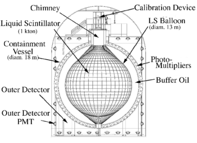
Figure 1: Schematic diagram of the KamLAND detector.

An event is recorded whenever 200 or more PMTs report a signal within 125 ns. A delayed-event window is then opened for 1 ms with a lower threshold of 120 tubes. The pulses are digitized by Analog Transient Waveform Digitizers (ATWDs). There are two ATWDs per PMT to reduce dead time during digitization.

The visible energy and position of each event is reconstructed from the collected charge and the hit pattern. The reconstruction algorithms are developed and tested using uniformly distributed spallation products following muons and using calibration data along the z-axis with ⁶⁸Ge, ⁶⁰Co, and ⁶⁵Zn gamma sources, and an AmBe neutron/gamma source. The calibration data are also used to estimate the conversion from visible energy to kinematic energy, taking into account particle-dependent non-linear effects due to quenching and cherenkov light production. The systematics on the energy scale is shown in the upper panel of Figure 2.

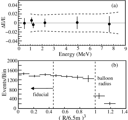
Figure 2: (a) Fractional error in energy reconstruction relative to the known source energies. The dashed line shows the systematic uncertainty in the energy scale. (b) Distribution in R³ of 2.2 MeV capture gammas from neutrons following muons. The ratio of events occurring inside the fiducial volume cut gives the fractional size of the fiducial volume.

Antineutrino events are selected according to the following criteria: time correlation 0.5 $\mu$s $<\Delta t<$ 660 $\mu$s; vertex correlation $\Delta R<$ 1.6 m; prompt event energy $E_{p}>$ 2.6 MeV; delayed event energy 1.8 MeV $<E_{d}<$ 2.6 MeV; spherical fiducial volume $R<$ 5 m; cylindrical radius $\rho>$ 1.2 m. The cut on $E_{p}$ eliminates $\bar{\nu}_{e}$ backgrounds from geological U/Th sources. The cylindrical radius cut removes backgrounds from thermometers deployed along the z-axis to monitor the scintillator. The total efficiency of these cuts was determined to be 78.3 $\pm$ 1.6%, and the residual accidental backgrounds, estimated using an off-coincidence time correlation window 20 $\mu$s $<\Delta t<$ 20 s, is negligible at $<10^{-5}$ events per day. The size of the fiducial volume is determined by counting the ratio of uniformly distributed spallation products that pass the fiducial volume cut. The distribution for spallation neutron capture gammas is given in the bottom panel of Figure 2.

The correlated backgrounds passing the $\bar{\nu}_{e}$ cuts are produced by cosmogenic spallation. An overburden of 2700 m.w.e. reduces the muon rate to $\sim$ 0.3 Hz. Muons are identified by their large energy deposit and outer detector activity, and the muon track is reconstructed from the PMT hit pattern. A 2 ms veto following muons eliminates backgrounds due to spallation neutrons and short lifetime spallation products. Long lifetime spallation products that mimic the $\bar{\nu}_{e}$ signal, such as ⁸He and ⁹Li, are removed by a 2 second veto in a 3 m radius around the muon track, plus a 2 second veto over the entire volume following muons with very high energy deposits ($\gtrsim$3 GeV). The residual correlated backgrounds, estimated from spallation event studies, time-since-last-muon distributions, and, for fast neutrons following muons not tagged by the OD, Monte Carlo simulations, is 1 $\pm$ 1 event in 145.1 days.

Figure 3 shows the distribution of the $\bar{\nu}_{e}$ candidates’ prompt and delayed energies. The delayed 2.2 MeV gamma cleanly separates $\bar{\nu}_{e}$ from the accidental coincidences clustered at small energies. The one event with $E_{d}\approx$ 5 MeV is consistent with neutron capture on carbon; such events are not considered in this analysis at a small cost in efficiency with negligible uncertainty.

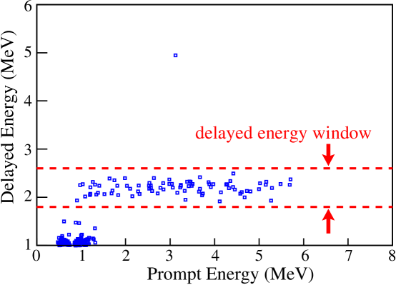
Figure 3: Prompt and delayed energies of $\bar{\nu}_{e}$ candidates.

The systematic uncertainties are listed in Table 1. The largest contribution to the systematics comes from the estimate of the fiducial mass ratio. The total uncertainty is 6.4%.

Table 1: Estimated systematic uncertainties (%).

Total LS mass	2.1	Reactor power	2.0
Fiducial mass ratio	4.1	Fuel composition	1.0
Energy threshold	2.1	Time lag	0.28
Efficiency of cuts	2.1	$\nu$ spectra [11]-[13]	2.5
Live time	0.07	Cross section [14]	0.2
Total systematic error			6.4%

For no oscillations, in 145.1 live-days we expect 86.8 $\pm$ 5.6 events with 1 $\pm$ 1 of these coming from backgrounds. The observed number of events is 54, giving a ratio $\frac{N_{obs}-N_{BG}}{N_{no~{}osc}}=0.611\pm$ 0.085 (stat) $\pm$ 0.041 (syst). This ratio is plotted vs. baseline for KamLAND and previous reactor experiments in Figure 4. The shaded region corresponds to the LMA MSW solution to the solar neutrino problem, with which the reactor experiments are in excellent agreement. ”Standard” $\bar{\nu}_{e}$ propagation is excluded at $>$ 99.95% C.L.

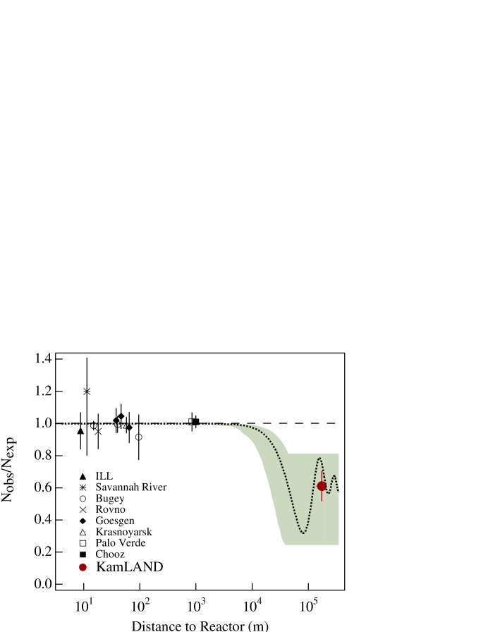
Figure 4: $N_{obs}/N_{no~{}osc}$ for reactor $\bar{\nu}_{e}$ experiments.

The positron energy spectrum is histogrammed in Figure 5. An unbinned maximum likelihood fit was performed and included terms for changes in the overall rate and shape of the spectrum at different points in $\Delta m^{2}-\sin^{2}2\theta$ parameter space. The best fit solution is plotted as the shaded histogram, and corresponds to $\Delta m^{2}=6.9\times 10^{-5}$ eV² and $\sin^{2}2\theta=1.0$. The regions in parameter space allowed at 95% C.L. are drawn in Figure 6. Also shown is the exclusion region in $\Delta m^{2}-\sin^{2}2\theta$ parameter space based on the KamLAND rate alone. Assuming CPT invariance (i.e. that $\nu$ and $\bar{\nu}$ masses are identical), all neutrino oscillation solutions to the solar neutrino problem are excluded except LMA. The KamLAND result divides LMA into two regions of higher and lower $\Delta m^{2}$. The sensitivity in $\sin^{2}2\theta$ is rather poor. Values of $\Delta m^{2}$ between the inclusion regions in general predict large distortions in the energy spectrum that were not observed and are hence disfavored. Constant suppression of the non-oscillated spectrum is consistent with the data at 53% C.L. The inclusion region extends to high $\Delta m^{2}$ where spectral distortions can not be distinguished with current statistics and energy resolution. An upper limit can be placed on $\Delta m^{2}$ using the non-observation of $\bar{\nu}_{e}$ disappearance by Palo Verde and Chooz.

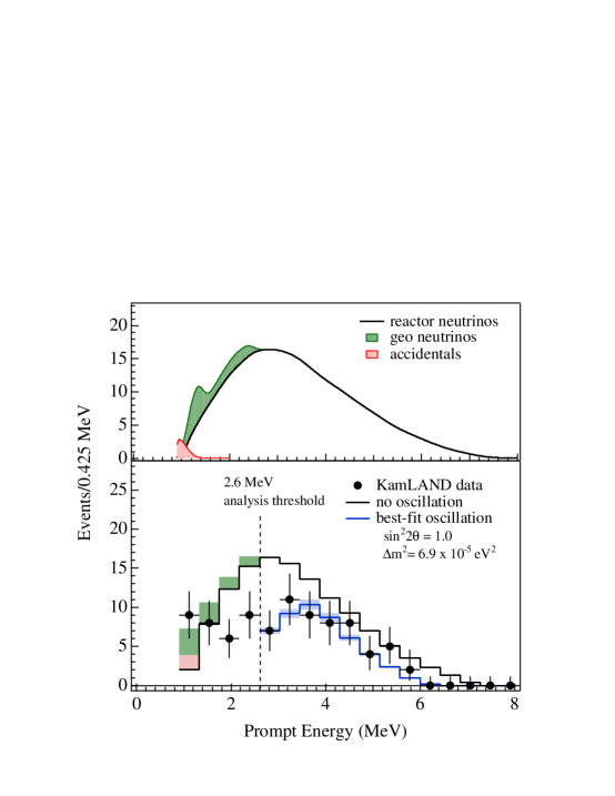
Figure 5: Prompt energy spectrum.

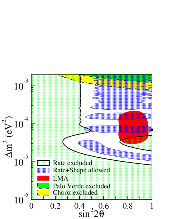
Figure 6: 95% inclusion region from KamLAND rate + shape.

4 Future of the KamLAND Reactor Measurement

Figure 7 shows the $\bar{\nu}_{e}$ flux at KamLAND from March 2002 through May 2003. In early 2003, Japanese utilities powered down their reactors for inspections and maintenance, resulting in a drop in the non-oscillated flux at KamLAND by about a factor of two. Such a drastic time variation will provide a more precise estimate of backgrounds, and depending on the ”true” values of $\Delta m^{2}$ and $\sin^{2}2\theta$, may also provide a time-varying spectral shape that will further restrict the inclusion regions in parameter space.

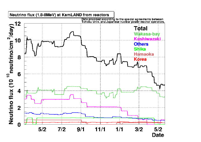
Figure 7: Time variation of the $\bar{\nu}_{e}$ flux at KamLAND.

The expected sensitivity of KamLAND for 5 years of data taking is shown in Figure 8 for two sets of parameters expected from KamLAND’s first results. KamLAND stands to provide exquisite sensitivity in $\Delta m^{2}$. However, further restrictions on $\sin^{2}2\theta$ will probably have to come from future solar neutrino experimental results.

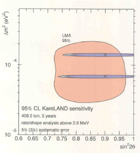
Figure 8: Expected KamLAND sensitivity for 5 years of data.

5 Future of Reactor Experiments

With the latest generation of solar and reactor experiments dawns a new age in precision neutrino oscillation physics. The next step in this exciting field will be to improve on current measurements and to measure some of the remaining unknown parameters in full three-flavor mixing. In addition to the three masses $m_{i}$, there are 6 free parameters in the mixing matrix $U_{li}$. It is possible to parameterize $U_{li}$ as follows:

$$U=U_{LMA}\times U_{atmospheric}\times U_{13}\times U_{\beta\beta}.$$ (10)

$$U_{LMA} = \left(\begin{array}[]{ccc}\cos\theta_{12}&\sin\theta_{12}&0\\ -\sin\theta_{12}&\cos\theta_{12}&0\\ 0&0&1\end{array}\right)$$ (14)

$$U_{atmospheric} = \left(\begin{array}[]{ccc}1&0&0\\ 0&\cos\theta_{23}&\sin\theta_{23}\\ 0&-\sin\theta_{23}&\cos\theta_{23}\end{array}\right)$$ (18)

$$U_{13} = \left(\begin{array}[]{ccc}\cos\theta_{13}&0&e^{-i\delta_{CP}}\sin\theta_{13}\\ 0&1&0\\ -e^{-i\delta_{CP}}\sin\theta_{13}&0&\cos\theta_{13}\end{array}\right)$$ (22)

$$U_{\beta\beta} = \left(\begin{array}[]{ccc}1&0&0\\ 0&e^{-i\frac{\alpha}{2}}&0\\ 0&0&e^{-i\frac{\alpha}{2}+i\beta}\end{array}\right)$$ (26)

$U_{atmospheric}$ and the value of $\Delta m^{2}_{23}$ has been measured by the Super-Kamiokande experiment.[21] $U_{\beta\beta}$ and the overall mass scale will require kinematical and neutrino-less double-$\beta$ decay measurements. KamLAND is playing a central role in determining $U_{LMA}$ as well as the value of $\Delta m^{2}_{12}$. Reactor experiments stand to play another role in neutrino oscillation, this time in the measurement of $U_{13}$.

Because $\Delta m^{2}_{12}\ll\Delta m^{2}_{23}$, it must be the case that $\Delta m^{2}_{13}\approx\Delta m^{2}_{23}$. A new generation of reactor experiments has been proposed to search for $\bar{\nu}_{e}$ disappearance at baselines of  1 km corresponding to this value of $\Delta m^{2}$. To improve on the mixing angle sensitivity achieved by Palo Verde and Chooz, proposals for reactor $\theta_{13}$ experiments include a large detector to reduce the statistical error, and also a second detector positioned very close ($\sim$100 m) to the reactor. The near detector would precisely measure the incident flux, allowing many of the flux calculation systematics to drop out. This also requires that the detectors be made identical and/or moveable. Sensitivity down to $\sin^{2}2\theta_{13}\approx 10^{-2}$ seems within grasp. Such experiments were first discussed by Mikaelyan and Sinev [22]; for a comprehensive list of references on this topic, please see the web site compiled by Heeger.[23]

6 Conclusion

KamLAND has observed, for the first time, disappearance of electron antineutrinos in a laboratory-style experiment. Assuming CPT invariance, this result excludes solar neutrino oscillation solutions except LMA at $>$ 99.95% C.L. Recall that the LMA solution to the solar neutrino problem is a region in oscillation parameter space allowed from the overlap of many experimental results using different techniques and with different thresholds. Moreover, LMA is an MSW solution for neutrinos, in which matter effects inside the sun drive the oscillations. It is significant that KamLAND, which uses yet another detection technique and is sensitive to vacuum oscillations of antineutrinos, gives oscillation parameters in agreement with LMA. These experiments are different in so many aspects, yet the physics of neutrino oscillation ties them together in a beautifully consistent theoretical framework.

7 Acknowledgements

The KamLAND experiment is supported by the Center of Excellence program of the Japanese Ministry of Education, Culture, Sports, Science and Technology, and the United States Department of Energy. The reactor data are provided courtesy of the following electric associations in Japan: Hokkaido, Tohoku, Tokyo, Hokuriku, Chubu, Kansai, Chugoku, Shikoku, and Kyushu Electric Power Companies, Japan Atomic Power Co., and Japan Nuclear Cycle Development Institute. Kamioka Mining and Smelting Company provided services for activities in the mine.

References

- [1] K. Eguchi et al., Phys. Rev. Lett. 90, 021802 (2003).
- [2] J.N. Bahcall and R. Davis, Science 191, 264 (1976); J.N. Bahcall, Neutrino Astrophysics (Cambridge University Press, Cambridge, UK, 1989); J.N. Bahcall, Astrophys. J 467, 475 (1996).
- [3] L. Wolfenstein, Phys. Rev. D 17, 2369 (1978).
- [4] S.P. Mikheev and A.Yu. Smirnov, Sov. J. Nucl. Phys. 42, 913 (1985).
- [5] B.T. Cleveland et al., Astrophys. J 496, 505 (1998).
- [6] GALLEX Collaboration, Phys. Lett. B 447, 127 (1999).
- [7] J.N. Abdurashitov et al., Phys. Rev. C 60, 055801 (1999).
- [8] Y. Fukuda et al., Phys. Rev. Lett. 77, 1683 (1996).
- [9] Super-Kamiokande Collaboration, Phys. Lett. B 539, 179 (2002).
- [10] Q.R. Ahmad et al., Phys. Rev. Lett. 89, 011302 (2002).
- [11] A.A. Hahn et al., Phys. Lett. B 218, 365 (1989).
- [12] K. Schreckenbach et al., Phys. Lett. B 160, 325 (1985).
- [13] P. Vogel et al., Phys. Rev. C 24, 1543 (1981).
- [14] P. Vogel and J. F. Beacom, Phys. Rev. D 60, 053003 (1999); radiative correction from A. Kurylov, et al., hep-ph/0211306.
- [15] F. Boehm et al., Phys. Rev. D 64, 112001 (2001).
- [16] M. Apollonio et al., EPJC 27, 331 (2003).
- [17] H. Kwon et al., Phys. Rev. D 24, 1097 (1981).
- [18] G. Zacek et al., Phys. Rev. D 34, 2621 (1986).
- [19] G.S. Vidyakin et al., JETP 59, 390 (1994).
- [20] B. Achkar et al., Nucl. Phys. B 434, 503 (1995); B. Achkar et al., Phys. Lett. B 374, 243 (1996).
- [21] Super-Kamiokande Collaboration, Phys. Lett. B 467, 185 (1999).
- [22] L.A. Mikaelyan and V.V. Sinev, Phys. Atom. Nucl. 63, 1002 (2001).
- [23] http://theta13.lbl.gov/references.html