Measurement of Branching Fractions of Color-Suppressed Decays
of the $\kern 2.15991pt\overline{\kern-2.15991ptB}{}^{0}$ Meson to $D^{(*)0}$$\pi^{0}$, $\mathbf{\mbox{$D^{(*)0}$}\eta}$, $\mathbf{\mbox{$D^{(*)0}$}\omega}$, and $\mathbf{\mbox{$D^{0}$}\eta^{\prime}}$

Abstract

Using a sample of $88.8\times 10^{6}$ $B\kern 1.79993pt\overline{\kern-1.79993ptB}{}$ events collected with the BABAR detector at the PEP-II storage rings at the Stanford Linear Accelerator Center, we measure the branching fractions of seven color-suppressed $B$-meson decays: ${\cal B}(\kern 1.79993pt\overline{\kern-1.79993ptB}{}^{0}\rightarrow D^{0}\pi^{0})$ $=(2.9\pm 0.2({\rm stat.})\pm 0.3({\rm syst.}))\times 10^{-4}$, ${\cal B}(\kern 1.79993pt\overline{\kern-1.79993ptB}{}^{0}\rightarrow D^{*0}\pi^{0})$ $=(2.9\pm 0.4({\rm stat.})\pm 0.5({\rm syst.}))\times 10^{-4}$, ${\cal B}(\kern 1.79993pt\overline{\kern-1.79993ptB}{}^{0}\rightarrow D^{0}\eta)$ $=(2.5\pm 0.2({\rm stat.})\pm 0.3({\rm syst.}))\times 10^{-4}$, ${\cal B}(\kern 1.79993pt\overline{\kern-1.79993ptB}{}^{0}\rightarrow D^{*0}\eta)$ $=(2.6\pm 0.4({\rm stat.})\pm 0.4({\rm syst.}))\times 10^{-4}$, ${\cal B}(\kern 1.79993pt\overline{\kern-1.79993ptB}{}^{0}\rightarrow D^{0}\omega)$ $=(3.0\pm 0.3({\rm stat.})\pm 0.4({\rm syst.}))\times 10^{-4}$, ${\cal B}(\kern 1.79993pt\overline{\kern-1.79993ptB}{}^{0}\rightarrow D^{*0}\omega)$ $=(4.2\pm 0.7({\rm stat.})\pm 0.9({\rm syst.}))\times 10^{-4}$, and ${\cal B}(\kern 1.79993pt\overline{\kern-1.79993ptB}{}^{0}\rightarrow D^{0}\eta^{\prime})$ $=(1.7\pm 0.4({\rm stat.})\pm 0.2({\rm syst.}))\times 10^{-4}$. We set the 90% confidence-level upper limit: ${\cal B}(\kern 1.79993pt\overline{\kern-1.79993ptB}{}^{0}\rightarrow D^{*0}\eta^{\prime})$ $<2.6\times 10^{-4}$. The channels $\kern 1.79993pt\overline{\kern-1.79993ptB}{}^{0}\rightarrow D^{*0}\eta$, $D^{*0}\omega$, and $D^{0}\eta^{\prime}$ are seen with more than five-sigma statistical significance. All of these branching fractions are significantly larger than theoretical expectations based on the “naive” factorization model.

I Introduction

Figure 1: The (a) color-allowed and (b) color-suppressed spectator tree diagrams for $\mbox{$\kern 1.79993pt\overline{\kern-1.79993ptB}{}^{0}$}\rightarrow D\ h$ decays.

Weak decays like $\mbox{$\kern 1.79993pt\overline{\kern-1.79993ptB}{}^{0}$}\rightarrow\mbox{$D^{(*)+}$}\mbox{$h^{-}$}$ can proceed through the emission of a virtual $W^{-}$, which then can materialize as a charged hadron ref:footnote1 . Because the $W^{-}$ carries no color, no exchange of gluons with the rest of the final state is required. Such decays are called color-allowed, though color-favored might be more apt. By contrast, decays like $\mbox{$\kern 1.79993pt\overline{\kern-1.79993ptB}{}^{0}$}\rightarrow\mbox{$D^{(*)0}$}\mbox{$h^{0}$}$ cannot occur in this fashion. The quark from the decay of the virtual $W^{-}$ must be combined with some anti-quark other than its partner from the $W^{-}$. However, other anti-quarks will have the right color to make a color singlet only one-third of the time. As a result, these decays are “color-suppressed”. The tree level diagrams for the color-allowed and color-suppressed decays are shown in Fig. 1.

Table 1: Prior measurements of branching fractions for $\kern 1.79993pt\overline{\kern-1.79993ptB}{}^{0}$ color-allowed and color-suppressed decays. When two uncertainties are given, the first uncertainty is statistical and the second systematic. We also quote the 90% confidence upper limits (UL) when the statistical significance of the measurement is less than four standard deviations.

$\kern 1.79993pt\overline{\kern-1.79993ptB}{}^{0}$ mode		$\mbox{${\cal B}$}\ (\times 10^{-4})$		UL ($\times 10^{-4}$)
$D^{+}\pi^{-}$		$26.8\pm 1.2\pm 2.7$ ref:cleoDpi		-
$D^{0}$$\pi^{0}$		$2.9\pm 0.5$ ref:PDG		-
$D^{\ast+}\pi^{-}$		$27.6\pm 2.1$ ref:PDG		-
$D^{*0}$$\pi^{0}$		$2.5\pm 0.7$ ref:PDG		-
$D^{+}\rho^{-}$		$78\pm 14$ ref:PDG		-
$\mbox{$D^{0}$}\rho^{0}$		$2.9\pm 1.0\pm 0.4$ ref:Belle2		-
$D^{\ast+}\rho^{-}$		$73\pm 15$ ref:PDG		-
$\mbox{$D^{*0}$}\rho^{0}$		-		$<5.1$ ref:Belle2
$\mbox{$D^{0}$}\eta$		$1.4^{+0.5}_{-0.4}\pm 0.3$ ref:Belle
$\mbox{$D^{*0}$}\eta$		$2.0^{+0.9}_{-0.8}\pm 0.4$ ref:Belle		$<2.6$ ref:PDG
$\mbox{$D^{0}$}\omega$		$1.8\pm 0.5^{+0.4}_{-0.3}$ ref:Belle		-
$\mbox{$D^{*0}$}\omega$		$3.1^{+1.3}_{-1.1}\pm 0.8$ ref:Belle		$<7.4$ ref:PDG
$\mbox{$D^{0}$}\eta^{\prime}$		-		$<9.4$ ref:PDG
$\mbox{$D^{*0}$}\eta^{\prime}$		-		$<14$ ref:PDG

The decays of $\kern 1.79993pt\overline{\kern-1.79993ptB}{}^{0}$ into $D^{(*)0}$$\pi^{0}$ have been observed by the CLEO collaboration ref:CLEO , while the $\kern 1.79993pt\overline{\kern-1.79993ptB}{}^{0}$ decays into $D^{(*)0}$$\pi^{0}$, $\mbox{$D^{0}$}\eta$, $\mbox{$D^{0}$}\omega$, and $\mbox{$D^{0}$}\rho^{0}$ have also been measured by the Belle collaboration ref:Belle ; ref:Belle2 . We present in Table 1 the prior measurements of branching fractions of the $\kern 1.79993pt\overline{\kern-1.79993ptB}{}^{0}$ color-allowed and color-suppressed decays. The level of color suppression can be estimated from the branching fractions for the $D^{(\ast)}\pi$ and $D^{(\ast)}\rho$ decay modes.

Since QCD calculations of decay rates from first principles are at present not possible, we must rely on models to describe the above processes. In an early model ref:BSW ; ref:Deandrea1 , the “naive” (or “generalized”) factorization model, which is very successful in describing charmed meson decays, the decay amplitudes of exclusive two-body non-leptonic weak decays of heavy flavor mesons are estimated by replacing hadronic matrix elements of four-quark operators in the effective weak Hamiltonian by products of current matrix elements. These current matrix elements are determined in terms of form factors describing the transition of the $B$ meson into the meson containing the spectator quark, and a factor proportional to a decay constant describing the creation of a single meson from the remaining quark–anti-quark pair. In this approach, the decay amplitudes corresponding to Figs. 1(a) and 1(b) are proportional to $a_{1}$ and $a_{2}$ ref:NeuSte , respectively, where the $a_{i}$ are effective QCD Wilson coefficients. As an example, using the naive factorization model, the decay amplitude for the $\mbox{$\kern 1.79993pt\overline{\kern-1.79993ptB}{}^{0}$}\rightarrow D^{+}\pi^{-}$ mode corresponding to Fig. 1(a) can be written as ref:NeuSte

$${\cal A}^{f}{(\mbox{$\kern 1.79993pt\overline{\kern-1.79993ptB}{}^{0}$}\rightarrow D^{+}\pi^{-})}=\\ i{{G_{F}}\over\sqrt{2}}V_{cb}V^{\ast}_{ud}(m^{2}_{B}-m^{2}_{D})a_{1}f_{\pi}F_{0}^{B\rightarrow D}(m^{2}_{\pi}),$$ (1)

while the decay amplitude for the $\mbox{$\kern 1.79993pt\overline{\kern-1.79993ptB}{}^{0}$}\rightarrow D^{0}\mbox{$\pi^{0}$}$ mode corresponding to Fig. 1(b) can be expressed as ref:NeuPet ; ref:ChengYang

$$\sqrt{2}{\cal A}^{f}{(\mbox{$\kern 1.79993pt\overline{\kern-1.79993ptB}{}^{0}$}\rightarrow D^{0}\mbox{$\pi^{0}$})}=\\ i{{G_{F}}\over\sqrt{2}}V_{cb}V^{\ast}_{ud}(m^{2}_{B}-m^{2}_{\pi})a_{2}f_{D}F_{0}^{B\rightarrow\pi}(m^{2}_{D}),$$ (2)

where $G_{F}$ is the Fermi coupling constant, $V_{cb}$ and $V_{ud}$ are CKM matrix elements, $f_{\pi}$ and $f_{D}$ are the decay constants of the $\pi$ and $D$ mesons, and $F_{0}^{B\rightarrow M}(q^{2})$ are the longitudinal form factors of the $B$-meson decays to $M$ mesons at momentum transfer $q^{2}$. The coefficients $a_{1}$ and $a_{2}$ are real in the absence of final-state interactions (FSI) and ideally would be process independent ref:BSW ; ref:Deandrea1 ; ref:NeuSte ; ref:NeuPet .

The color-allowed $\mbox{$\kern 1.79993pt\overline{\kern-1.79993ptB}{}^{0}$}\rightarrow D^{(*)+}(\pi^{-},\rho^{-},a_{1}^{-})$ and $B\rightarrow D^{(*)}D_{s}^{(*)}$ decays, the color-suppressed $B\rightarrow(c\mbox{$\overline{c}$})(K^{(*)},\pi)$ decays, and the mixed $B^{-}\rightarrow\mbox{$D^{(*)0}$}(\pi^{-},\rho^{-},a_{1}^{-})$ decays can all be accommodated by universal constants $a_{1}=1.1\pm 0.2$ and $a_{2}\simeq$ 0.2–0.3 ref:Beneke ; ref:NeuSte ; ref:KKW ; ref:PDG . This no longer holds for color-suppressed $B$ decays with one $c$-quark only, like $D^{(*)}\pi$, where measurements listed in Table 1 are inconsistent with a universal value of $a_{2}$ in the absence of FSI ref:NeuPet . The naive factorization model ref:Beneke ; ref:NeuSte ; ref:NeuPet ; ref:Chua ; ref:Rosner ; ref:Deandrea ; ref:ChRos predicts too small values for the branching fractions of the color-suppressed modes, in the range $(0.3$–$1.7)\times 10^{-4}$ and corresponding to a factor $(a_{2}/a_{1})^{2}\simeq$ 0.03–0.09.

Final state interactions, however, may change this picture significantly and, thus, may increase substantially these rates, as rescattering effects can connect the final states shown in Fig. 1(a) and Fig. 1(b) (see, for example, Ref. ref:Chua ). Similar effects have already in the past completely changed the conclusions of the models that describe non-leptonic $D^{0}$ decays, especially for decay modes such as $\mbox{$D^{0}$}\rightarrow\mbox{$\kern 1.79993pt\overline{\kern-1.79993ptK}{}^{0}$}\mbox{$\pi^{0}$}$ ref:Lipkin . Therefore, in the case of large FSI, a description in terms of isospin amplitudes is more appropriate and will be used in Sec. IX.2 to discuss our results.

This situation is an impetus for higher precision results and the investigation of additional channels that might provide clues to the underlying mechanisms. In this paper we report on the branching fraction measurements of the seven color-suppressed $\kern 1.79993pt\overline{\kern-1.79993ptB}{}^{0}$-meson decays to $D^{(*)0}$$\pi^{0}$, $\mbox{$D^{(*)0}$}\eta$, $\mbox{$D^{(*)0}$}\omega$, and $\mbox{$D^{0}$}\eta^{\prime}$. We also report on a search for the $\mbox{$\kern 1.79993pt\overline{\kern-1.79993ptB}{}^{0}$}\rightarrow\mbox{$D^{*0}$}\eta^{\prime}$ decay. These results are based upon an integrated luminosity equivalent to $88.8\times 10^{6}$ $B\kern 1.79993pt\overline{\kern-1.79993ptB}{}$ events. This corresponds to about nine times that used for the earlier measurement by CLEO ref:CLEO ($9.7\times 10^{6}$ $B\kern 1.79993pt\overline{\kern-1.79993ptB}{}$ events) and about four times that used for the earlier measurements by Belle ref:Belle ($23.1\times 10^{6}$ $B\kern 1.79993pt\overline{\kern-1.79993ptB}{}$ events). Recently, with $31.3\times 10^{6}$ $B\kern 1.79993pt\overline{\kern-1.79993ptB}{}$ events, the Belle collaboration has reported branching fraction measurements for $\mbox{$\kern 1.79993pt\overline{\kern-1.79993ptB}{}^{0}$}\rightarrow\mbox{$D^{(*)0}$}\pi^{+}\pi^{-}$ decays, including the $\mbox{$D^{0}$}\rho^{0}$ mode, as already discussed, and the investigation of the $\mbox{$D^{*0}$}\rho^{0}$ channel ref:Belle2 . We present the first measurement of the $\mbox{$\kern 1.79993pt\overline{\kern-1.79993ptB}{}^{0}$}\rightarrow\mbox{$D^{*0}$}\eta$, $\mbox{$D^{*0}$}\omega$, and $\mbox{$D^{0}$}\eta^{\prime}$ modes with more than five-sigma statistical significance.

II The BABAR detector and data sample

The BABAR detector is located at the PEP-II $e^{+}e^{-}$ storage rings operating at the Stanford Linear Accelerator Center. At PEP-II 9.0-GeV electrons collide with 3.1-GeV positrons to produce a center-of-mass energy of $10.58\,\mbox{\rm GeV}$, the mass of the $\mathchar 28935\relax{(4S)}$. The data used in this analysis were collected with the BABAR detector and correspond to an integrated luminosity of $81.9\,\mbox{${\rm fb^{-1}}$}$ recorded at the $\mathchar 28935\relax{(4S)}$ resonance.

The BABAR detector is described in detail in Ref. ref:babar . Surrounding the interaction point is a 5-layer double-sided silicon vertex tracker (SVT), which gives precision spatial information in three dimensions for charged particles and measures their energy loss $(\mbox{$dE/dx$})$. The SVT is the primary detection device for low-momentum charged particles. Outside the SVT, a 40-layer drift chamber (DCH) provides measurements of the polar angles and of the transverse momentum ($p_{T}$) of charged particles with respect to the beam direction, together with the SVT. The resolution of the $p_{T}$ measurement for tracks with momenta above $1\,\mbox{${\rm GeV}/c$}$ is $\sigma_{\mbox{$p_{T}$}}/\mbox{$p_{T}$}=0.13\%\times\mbox{$p_{T}$}+0.45\%$, where $p_{T}$ is measured in ${\rm GeV}/c$. The drift chamber measures $dE/dx$ with a precision of 7.5%. Beyond the outer radius of the DCH is a detector of internally reflected Cherenkov radiation (DIRC), which is used primarily for charged-hadron identification. The detector consists of quartz bars in which Cherenkov light is produced when relativistic charged particles traverse the material. The light is internally reflected along the length of the bar into a water-filled volume mounted on one end of the detector. The Cherenkov rings expand in the water volume and are measured with an array of photomultiplier tubes mounted on its outer surface. A CsI(Tl) crystal electromagnetic calorimeter (EMC) is used to detect photons and neutral hadrons, as well as to identify electrons. The resolution of the calorimeter can be expressed as $\sigma_{E}/E=2.3\%/(E)^{\frac{1}{4}}\oplus 1.9\%$, where $E$ is measured in GeV. The EMC detects photons with energies down to $20\,\mbox{\rm MeV}$. The EMC is surrounded by a superconducting solenoid, which produces at 1.5-T magnetic field. The instrumented flux-return (IFR) consists of multiple layers of resistive plate chambers (RPC) interleaved with the flux-return iron. The IFR is used in the identification of muons and long-lived neutral hadrons.

Signal and generic background Monte Carlo events are generated using the BABAR particle decay simulation package ref:Lange , the “EvtGen” package. The interactions of the generated particles traversing the detector are simulated using the GEANT4 ref:GEANT program. Beam-induced backgrounds, which varied from one data-taking period to the next, are taken into account in the simulation of the detector response. This is done by adding the signals generated by these beam-induced backgrounds to the simulation of the various physics events.

III Particle reconstruction and Counting of $B\kern 1.79993pt\overline{\kern-1.79993ptB}{}$ events

Charged-particle tracks are reconstructed from measurements in the SVT and/or the DCH. The tracks must have at least 12 hits in the DCH and $\mbox{$p_{T}$}>100$ ${\rm MeV}/c$ ref:footnote2 . In the case of the tracks used to reconstruct $\rho^{\pm}$ mesons, we also use tracks reconstructed with the SVT alone (see Sec. IV.2.1). The tracks must extrapolate to within $20\,\mbox{\rm mm}$ of the $e^{+}$$e^{-}$ interaction point in the plane transverse to the beam axis and to within $50\,\mbox{\rm mm}$ along the beam axis. Charged-kaon candidates are identified using a likelihood function that combines ${\rm d}E/{\rm d}x$ and DIRC information. The likelihood function is used to define tight and loose kaon criteria as pion vetos. To satisfy the tight kaon criterion, the track must also have $p>250$ ${\rm MeV}/c$ and make an angle with respect to the electron beam direction, which is used as the reference axis for all the polar angles, between 0.45 and $2.50\,\mbox{\rm rad}$ so that the candidate is within the fiducial region of the DIRC. Photons are identified by energy deposits in contiguous crystals in the EMC. Each photon must have an energy greater than 30 MeV and a lateral shower shape consistent with that of an electromagnetic shower.

The measurement of branching fractions depends upon an accurate measurement of the number of $B\kern 1.79993pt\overline{\kern-1.79993ptB}{}$ meson pairs in the data sample. We find the number of $B\kern 1.79993pt\overline{\kern-1.79993ptB}{}$ pairs by comparing the rate of spherical multi-hadron events in data recorded on the $\mathchar 28935\relax{(4S)}$  resonance to that in data taken off-resonance. This latter data sample is collected 40 MeV below the $\mathchar 28935\relax{(4S)}$ resonance and corresponds to an integrated luminosity of about $10\,\mbox{${\rm fb^{-1}}$}$.

The purity of the multi-hadrons events is enhanced by requiring the events to pass selection criteria based on all tracks (including those reconstructed in the SVT only), detected in the fiducial region $0.41<\theta<2.54\ \mbox{\rm rad}$ and on neutral clusters with an energy greater than 30 MeV, in the fiducial region $0.410<\theta<2.409\ \mbox{\rm rad}$:

• There must be at least three tracks in the fiducial region. The total energy of the charged and neutral particles in the fiducial region must be greater than 4.5 GeV.

• The ratio of the second to the zeroth Fox-Wolfram moment ref:FoxWolf must be less than 0.5. All tracks and neutral clusters defined above are used.

• The event vertex must be within $5\,\mbox{\rm mm}$ of the nominal beam-spot position in the plane transverse to the beam and within $60\,\mbox{\rm mm}$ along the beam direction.

These requirements are about 95.4% efficient for $B\kern 1.79993pt\overline{\kern-1.79993ptB}{}$ events as estimated from Monte Carlo simulation. The systematic uncertainty on the number of $B\kern 1.79993pt\overline{\kern-1.79993ptB}{}$ events is 1.1%.

IV Meson candidate selection

IV.1 General considerations

The color-suppressed $\kern 1.79993pt\overline{\kern-1.79993ptB}{}^{0}$ meson decay modes are reconstructed from $D^{0}$ or $D^{*0}$ meson candidates that are combined with light neutral-meson candidates $h^{0}$ ($\pi^{0}$, $\eta$, $\omega$, and $\eta^{\prime}$). Events are required to pass the selection criteria used for $B\kern 1.79993pt\overline{\kern-1.79993ptB}{}$ counting listed in Sec. III. Additional requirements discussed below are applied to the signal sample.

We combine tracks and/or neutral clusters to form candidates for the mesons produced in the $B$ decays. Vertex constraints are applied to charged daughters before computing their invariant masses. At each step in the decay chain we require that mesons have masses consistent with their assumed particle type. If daughter particles are produced in the decay of a parent meson with a natural width that is small relative to the reconstructed width, we constrain the meson’s mass to its nominal value. This fitting technique improves the resolution of the energy and the momentum of the $\kern 1.79993pt\overline{\kern-1.79993ptB}{}^{0}$ candidates as they are calculated from improved energies and momenta of the $D^{(*)0}$ and $h^{0}$.

We select $D^{*0}$, $D^{0}$, $h^{0}$, and $\kern 1.79993pt\overline{\kern-1.79993ptB}{}^{0}$ candidates using only well-understood discriminating variables in order to reduce the systematic uncertainties for the branching fraction measurements. We choose selection criteria that maximize the quality factor $Q=S/\sqrt{S+B}$, where $S$ and $B$ are the expected number of signal and background events. The values of $S$ and $B$ are estimated from signal and background Monte Carlo simulation and data in the signal sidebands, but not from data in the signal regions. When optimizing the cuts, the values of $S$ have been estimated using the previous branching fraction measurements obtained by the CLEO ref:CLEO and Belle ref:Belle collaborations. For the $\mbox{$D^{(*)0}$}\eta^{\prime}$ analyses, a conservative value for the branching fractions equal to $10^{-4}$ has been assumed. In most cases we find that $Q$ does not change significantly when selection criteria are varied near their optimal values. This allows us to choose selection criteria that are common to most final states.

IV.2 Selection of $h^{0}$ and $\rho^{\pm}$ candidates

The momentum of the $h^{0}$ candidate must satisfy the condition $1.3<p^{\ast}<3.0$ GeV/c. This requirement is loose enough that various sources of background populate the sidebands of the signal region. These sidebands are used in the background estimate for the signal.

IV.2.1 $\pi^{0}$ and $\rho^{\pm}$ selection

The $\pi^{0}$ meson is reconstructed from photon pairs. We consider three sources of $\pi^{0}$ with decreasing momenta: $\pi^{0}$ originating from $\kern 1.79993pt\overline{\kern-1.79993ptB}{}^{0}$ decays, from $D^{0}$, $\eta$, and $\omega$ decays, and directly from $D^{*0}$ decays. The latter two sources are discussed below. The mass resolution of $\pi^{0}$ candidates from $\kern 1.79993pt\overline{\kern-1.79993ptB}{}^{0}$ decays with momenta $p^{\ast}$ near 2 ${\rm GeV}/c$ is dominated by the uncertainty in the opening angle between the two photons and is approximately 8 ${\rm MeV}/c^{2}$.

These $\pi^{0}$s are also combined with charged pions to attempt the reconstruction of $\rho^{-}$ mesons. The charged pions are not required to satisfy our regular selection criteria for tracks. Thus we retain also low momentum charged pions that are reconstructed with the SVT alone. A $\mbox{$\pi^{0}$}\pi^{-}$ pair is selected if its mass is reconstructed within 250 ${\rm MeV}/c^{2}$ of the nominal $\rho^{-}$ meson mass. The $\rho^{-}$ candidates are used to reconstruct the color-allowed $\mbox{$B^{-}$}\rightarrow\mbox{$D^{(*)0}$}\rho^{-}$ decays that form a significant background for $\mbox{$\kern 1.79993pt\overline{\kern-1.79993ptB}{}^{0}$}\rightarrow\mbox{$D^{(*)0}$}\mbox{$\pi^{0}$}$. The color-allowed decays have branching fractions about fifty times that for $\mbox{$\kern 1.79993pt\overline{\kern-1.79993ptB}{}^{0}$}\rightarrow\mbox{$D^{(*)0}$}\mbox{$\pi^{0}$}$ and they mimic the latter through an asymmetric $\rho^{-}$ decay in which the $\pi^{0}$ carries most of the available energy. We veto events with a reconstructed $\mbox{$B^{-}$}\rightarrow\mbox{$D^{(*)0}$}\mbox{$\rho^{-}$}$. A discussion of the veto is deferred until Secs. VI.1 and B.

IV.2.2 $\eta$ selection

The $\eta$ candidate is reconstructed in the $\gamma\gamma$ and $\pi^{+}$$\pi^{-}$$\pi^{0}$ decay modes. The branching fraction in the $\gamma\gamma$ mode is almost twice as large as that of the $\pi^{+}$$\pi^{-}$$\pi^{0}$ decay channel and the efficiency for the $\gamma\gamma$ mode is greater since there are fewer particles to detect.

In the $\gamma\gamma$ decay mode we require that the photons have energies greater than 200 MeV. A photon is not used if it can be paired with another photon with energy greater than 150 MeV to form a $\pi^{0}$ candidate with an invariant mass in the range 120–150 ${\rm MeV}/c^{2}$. The mass resolution for $\eta\rightarrow\gamma\gamma$ is approximately 15 ${\rm MeV}/c^{2}$.

In the $\pi^{+}$$\pi^{-}$$\pi^{0}$ decay mode, the $\eta$ meson is reconstructed employing a vertex constraint that requires a $\chi^{2}$ probability greater than 0.1%. To reduce combinatorial background the charged-pion candidates must have momentum greater than 250 ${\rm MeV}/c$ and they must fail the tight kaon criterion, while the $\pi^{0}$ must have an energy greater than 300 MeV and a mass in the range 115–150 ${\rm MeV}/c^{2}$. The mass resolution for $\eta\rightarrow\mbox{\mbox{$\pi^{+}$}\mbox{$\pi^{-}$}\mbox{$\pi^{0}$}}$ is approximately 4 ${\rm MeV}/c^{2}$.

IV.2.3 $\omega$ selection

The $\omega$ meson is reconstructed in its $\pi^{+}$$\pi^{-}$$\pi^{0}$ decay mode, employing a vertex constraint that requires a $\chi^{2}$ probability greater than 0.1%. To reduce combinatorial background, the charged pion candidates must have momentum greater than 200 ${\rm MeV}/c$ and they must fail the tight kaon criterion, while the $\pi^{0}$ must have an energy greater than 250 MeV and a mass in the range 120–150 ${\rm MeV}/c^{2}$. The mass resolution of the $\omega$ is dominated by its natural width of approximately $10\,\mbox{${\rm MeV}/c^{2}$}$. The use of additional angular properties in the $\omega$ meson decays will be described in Sec. IV.4.1.

IV.2.4 $\eta^{\prime}$ selection

We reconstruct the $\eta^{\prime}$ meson in its $\mbox{$\mbox{$\pi^{+}$}\mbox{$\pi^{-}$}\eta$}(\rightarrow\gamma\gamma)$ decay mode. The product of the branching fractions of secondary decays in this channel is 17.5% ref:PDG . This limits the signal efficiency, so a separate event selection for $D^{(*)0}$$\eta^{\prime}$ is used. We use the $\mbox{$\pi^{+}$}\mbox{$\pi^{-}$}\eta$ decay mode rather than the dominant $\rho^{0}\gamma$ mode as it provides a much cleaner signal.

The two photons used to reconstruct the $\eta$ candidate are required to have energies greater than 100 MeV. A photon is not used to reconstruct the $\eta$ meson if it can be paired with another photon with energy greater than 100 MeV to form a $\pi^{0}$ candidate with mass in the range 120–150 ${\rm MeV}/c^{2}$. We select $\eta$ candidates with a mass in the range 495–600 ${\rm MeV}/c^{2}$. To obtain the highest possible signal efficiency we rely on the high purity of the signal and impose neither a momentum nor any particle-identification requirement on the charged pions. For the same reason, a vertex constraint is applied to the $\pi^{+}$$\pi^{-}$ pair when computing the energy and the momentum of an $\eta^{\prime}$ meson candidate, but there is no requirement on the $\chi^{2}$ probability of the vertex. The mass resolution for $\eta^{\prime}\rightarrow\mbox{$\mbox{$\pi^{+}$}\mbox{$\pi^{-}$}\eta$}(\rightarrow\gamma\gamma)$ is approximately 4 ${\rm MeV}/c^{2}$.

IV.3 Selection of $D^{0}$ and $D^{*0}$ candidates

The momentum of the $D^{(*)0}$ mesons must satisfy the condition $p^{\ast}>1.5$ GeV/c. As for the light neutral-hadron selection, this requirement retains sidebands, which can be used to evaluate backgrounds.

IV.3.1 $\mbox{$D^{0}$}\to\mbox{$\mbox{$K^{-}$}\mbox{$\pi^{+}$}$}$, $K^{-}$$\pi^{+}$$\pi^{0}$, and $K^{-}$$\pi^{+}$$\pi^{+}$$\pi^{-}$ selection

The $D^{0}$ mesons are reconstructed in three decay modes: $K^{-}$$\pi^{+}$, $K^{-}$$\pi^{+}$$\pi^{0}$, and $K^{-}$$\pi^{+}$$\pi^{+}$$\pi^{-}$. The $\chi^{2}$ probability for the vertex fit of the charged pions is required to be greater than 0.1%. In the $K^{-}$$\pi^{+}$ final state the kaon candidate must satisfy the pion veto requirement, while in the $K^{-}$$\pi^{+}$$\pi^{0}$ and $K^{-}$$\pi^{+}$$\pi^{+}$$\pi^{-}$ final states the kaon candidate must satisfy the tight kaon criterion because of the increased background present in these combinations. All pion candidates must fail the tight kaon criterion.

To reduce combinatorial background in the $K^{-}$$\pi^{+}$$\pi^{0}$ final state we use the results of the Fermilab E691 experiment ref:DaliKpipi0 , which determined the distribution of events in the Dalitz plot. This distribution is dominated by the two possible $K^{*}$ resonances ($K^{*0}\rightarrow\mbox{$K^{-}$}\pi^{+}$ or $K^{*-}\rightarrow\mbox{$K^{-}$}\mbox{$\pi^{0}$}$) and by the $\mbox{$\rho^{+}$}(\rightarrow\mbox{$\pi^{+}$}\mbox{$\pi^{0}$})$ resonance. We select only those events that fall in the enhanced regions of the Dalitz plot as determined by experiment E691. Reconstructed $\pi^{0}$ mesons are required to have masses in the range 115–150 ${\rm MeV}/c^{2}$. The mass resolution is approximately 6.5 ${\rm MeV}/c^{2}$. To increase the signal purity only $\pi^{0}$ mesons with energy greater than 300 MeV, as defined in the laboratory frame, are retained.

The $D^{0}$ mass resolutions are approximately 6.7, 10.7, and 5.0 ${\rm MeV}/c^{2}$ for the $K^{-}$$\pi^{+}$, $K^{-}$$\pi^{+}$$\pi^{0}$, and $K^{-}$$\pi^{+}$$\pi^{+}$$\pi^{-}$ decay modes, respectively.

IV.3.2 $\mbox{$D^{*0}$}\to\mbox{$D^{0}$}\mbox{$\pi^{0}$}$ selection

The $D^{*0}$ mesons are reconstructed in the $D^{0}$$\pi^{0}$ decay mode. The $D^{0}$ candidates are selected as described above. The $\pi^{0}$ candidates are required to have momenta that satisfy the condition $70<p^{\ast}<300$ MeV/c and a mass in the range 115–150 ${\rm MeV}/c^{2}$. The mass resolution for the soft $\pi^{0}$ daughter is approximately 6.5 ${\rm MeV}/c^{2}$. The resolution of the $D^{*0}$–$D^{0}$ mass difference is approximately 1 ${\rm MeV}/c^{2}$.

IV.4 Selection of $B$ candidates

IV.4.1 Event shape and angular distributions

Both $B\kern 1.79993pt\overline{\kern-1.79993ptB}{}$ events and $u$, $d$, $s$, and $c$ quark-antiquark events contribute to the combinatorial background that does not peak near the nominal $B$ mass. To reject $u$, $d$, $s$, and $c$ components we use shape variables and angular distributions that distinguish these from the signal $B\kern 1.79993pt\overline{\kern-1.79993ptB}{}$ events.

Because the $u$, $d$, $s$, and $c$ continuum events are jet-like, while $B$ meson decays produce spherical events, we can suppress them by requiring that the ratio of the second to the zeroth Fox-Wolfram moment ref:FoxWolf must be less than 0.5 as described in Sec. III. For each reconstructed $\kern 1.79993pt\overline{\kern-1.79993ptB}{}^{0}$ candidate we compute the thrust and sphericity axes of both the candidate and the rest of the event, using only the tracks and neutral clusters as defined in Sec. III. We define the angles $\theta_{\rm thr}$ and $\theta_{\rm sph}$ between the axes of the $\kern 1.79993pt\overline{\kern-1.79993ptB}{}^{0}$ candidate and the rest of the event. The distributions of $|\cos{\mbox{$\theta_{\rm thr}$}}|$ and $|\cos{\mbox{$\theta_{\rm sph}$}}|$ peak near 1.0 for $u$, $d$, $s$, and $c$ background while they are nearly flat for $B$ decays. Thus we require at least one of the conditions $|\cos{\mbox{$\theta_{\rm sph}$}}|<0.85$ or $|\cos{\mbox{$\theta_{\rm thr}$}}|<0.85$ to be true for the $D^{(*)0}$$\pi^{0}$, $\mbox{$D^{(*)0}$}\eta$, and $\mbox{$D^{(*)0}$}\omega$ modes. Since the two angles $\theta_{\rm thr}$ and $\theta_{\rm sph}$ are strongly but not completely correlated for signal events, the relative signal efficiency for this requirement is close to 92%. This is larger than the relative signal efficiency of about 85% if only the requirement $|\cos{\mbox{$\theta_{\rm thr}$}}|<0.85$ is applied, while the background rejection is about the same.

For the $D^{(*)0}$$\pi^{0}$, $\mbox{$D^{(*)0}$}\eta$, and $\mbox{$D^{(*)0}$}\omega$ final states we also take advantage of the $\sin^{2}{\mbox{$\theta_{\rm B^{\ast}}$}}$ distribution of the polar angle $\theta_{\rm B^{\ast}}$. This quantity is the angle between the $B$ momentum vector and the beam axis in the $\mathchar 28935\relax{(4S)}$ rest frame. Therefore we only keep the candidates that satisfy $|\cos{\mbox{$\theta_{\rm B^{\ast}}$}}|<0.8$ as the distribution is almost flat in $|\cos{\mbox{$\theta_{\rm B^{\ast}}$}}|$ for combinatorial background.

For the $\mbox{$D^{(*)0}$}\eta^{\prime}$ channels, we have seen that the event yield is expected to be small. In order to keep the signal acceptance as high as possible, we use a more complex scheme. We require $|\cos{\mbox{$\theta_{\rm thr}$}}|<0.9$ and then calculate a Fisher discriminant ($\cal F$) that combines eleven variables ref:CLEOCharmless . Two of these are the two polar angles $\theta_{\rm B^{\ast}}$ and $\theta_{\rm T}$, where $\theta_{\rm T}$ is the angle between the $B$ candidate thrust axis and the beam axis in the $\mathchar 28935\relax{(4S)}$ rest frame. The other nine are the scalar sums of the energies of all charged tracks and neutral showers (except those used in the $B$ candidate reconstruction) binned in nine $10^{\circ}$ polar angle intervals relative to the $B$ candidate thrust axis. The separation between the means of the signal and $q\bar{q}$ background distributions of the ${\cal F}$ variable is 1.2–1.3 times the width of either distribution.

For the $\mbox{$D^{0}$}\omega$ channel where the $\omega$ is necessarily longitudinally polarized, we use the properties of the distributions of two additional angles. The angle $\theta_{\rm N}$ is the angle between the normal to the plane of the three daughter pions in the $\omega$ center-of-mass frame and the line-of-flight of the $B$-meson in the $\omega$ rest frame. The angle $\theta_{\rm D}$ is the angle, in the rest frame of one dipion, between the third pion and either of the other two. The signal events are distributed as $\cos^{2}{\mbox{$\theta_{\rm N}$}}$ and $\sin^{2}{\mbox{$\theta_{\rm D}$}}$, while the corresponding $\cos{\mbox{$\theta_{\rm N}$}}$ and $\cos{\mbox{$\theta_{\rm D}$}}$ distributions are nearly flat for combinatorial background. We select only events in a region of the three-dimensional parameter space of the angles $\theta_{\rm B^{\ast}}$, $\theta_{\rm N}$, and $\theta_{\rm D}$ that has high signal efficiency. This region is defined by

$$\cos{\mbox{$\theta_{\rm D}$}}^{2}+\cos{\mbox{$\theta_{\rm B^{\ast}}$}}^{2}<0.64,$$ (3)

$${\left({\cos{\mbox{$\theta_{\rm D}$}}\over 0.8}\right)}^{2}+{\left({|\cos{\theta_{\rm N}}|-1.0\over 0.5}\right)}^{2}<1,$$ (4)

and

$${\left({\cos{\mbox{$\theta_{\rm B^{\ast}}$}}\over 0.8}\right)}^{2}+{\left({|\cos{\theta_{\rm N}}|-1.0\over 0.5}\right)}^{2}<1.$$ (5)

In the $\mbox{$D^{*0}$}\omega$ channel, the $\omega$ polarization is not known a priori and we apply only the requirement given by Eq. (3).

For the $D^{*0}$$h^{0}$, $\mbox{$h^{0}$}=\mbox{$\pi^{0}$}$, $\eta$, and $\eta^{\prime}$ modes where the $D^{*0}$ is longitudinally polarized, we use the angular decay distribution to reject combinatorial background. The angle $\theta_{\rm hel}$ is defined as the angle between the line-of-flight of the $D^{0}$ and the one of the $D^{*0}$, both evaluated in the $D^{*0}$ rest frame. The distribution is almost flat in $\cos{\mbox{$\theta_{\rm hel}$}}$ for combinatorial background, while signal events are distributed as $\cos^{2}{\mbox{$\theta_{\rm hel}$}}$. For the $D^{*0}$$\pi^{0}$ and $\mbox{$D^{*0}$}\eta$ channels we require

$${\left({\cos{\mbox{$\theta_{\rm B^{\ast}}$}}\over 0.8}\right)}^{2}+{\left({|\cos{\mbox{$\theta_{\rm hel}$}}|-1.0\over 0.6}\right)}^{2}<1.$$ (6)

For the $\mbox{$D^{*0}$}\eta^{\prime}$ final state we only require $|\cos{\mbox{$\theta_{\rm hel}$}}|>0.4$ since the angle $\theta_{\rm B^{\ast}}$ is already included in the definition of $\cal F$.

IV.4.2 Multiple $B$ candidates

After applying the above selection criteria, a small fraction of events have more than one $B$ candidate. The average multiplicity of $B$ candidates for the data events is between 1.01 and 1.18, depending on the $D^{0}$ decay mode. The average multiplicity is slightly higher for the $D^{*0}$$h^{0}$ modes than for the $D^{0}$$h^{0}$ modes. With the exception of the $\mbox{$D^{(*)0}$}\eta^{\prime}$ final states we select the $B$ candidate with the lowest value of

$$\mbox{$\chi^{2}$}_{B}=\left({\frac{m_{D}-m^{\rm nom}_{D}}{\sigma_{m_{D}}}}\right)^{2}+\left({\frac{m_{h}-m^{\rm nom}_{h}}{\sigma_{m_{h}}}}\right)^{2}+$$

$$\left({\frac{\Delta m_{D^{\ast}D}-\Delta m^{\rm nom}_{D^{\ast}D}}{\sigma_{\Delta m_{D^{\ast}D}}}}\right)^{2},$$ (7)

where $\sigma_{m_{D}}$ and $\sigma_{m_{h}}$ are the resolutions of the measured $D^{0}$ and $h^{0}$ masses. The last term in the equation is only present for $D^{*0}$ decays and $\sigma_{\Delta m_{D^{\ast}D}}$ is the average resolution of the measured $D^{*0}$–$D^{0}$ mass difference. The mass resolutions depend on the decay modes and are slightly different for data and Monte Carlo simulation. Each of the three terms is found to be approximately Gaussian with mean value near zero and standard deviation near one.

In order to reduce combinatorial backgrounds, we require that each of the terms in Eq. (7) is less than $2.5^{2}$ (a $\pm\ 2.5\,\sigma$ requirement). In the case of the $\omega$ mesons, the candidates must have a reconstructed invariant mass within $25$ ${\rm MeV}/c^{2}$ ($\pm\ 2.5$ times the $\omega$ natural width) of the nominal value.

For the $\mbox{$D^{(*)0}$}\eta^{\prime}$ channels, the signal acceptance is relatively lower than for other modes, but the background level is also much smaller. Therefore we keep all the candidates in the events and weight them by $1/N$ where $N$ is the number of $B$ candidates in the event. In order to reduce the combinatorial background for these two channels the invariant mass of the $\eta^{\prime}$ candidate is required to be within $2.5\,\sigma$ of its nominal value. The $D^{0}$ candidates are required to have a reconstructed mass within 2–3 $\sigma$ (depending on the decay mode) of their nominal value. We reject $D^{*0}$ candidates whose $D^{*0}$–$D^{0}$ mass difference is not within $3\,\sigma$ of its nominal value.

Table 2: The number of candidates (${\cal N}_{\rm cand}$), the number of non-peaking (${\cal N}_{\rm npb}$) and peaking (${\cal N}_{\rm pb}$) background events, the number of cross-feed (${\cal N}_{\rm CF}$) background events from other color-suppressed modes, the number of signal events ($S$) after peaking and cross-feed backgrounds are subtracted, and the statistical significance of the signals ($S/\sqrt{S+{\cal N}_{\rm bckgd}}$). We obtain ${\cal N}_{\rm npb}$ from a fit to the data $m_{\rm ES}$ distribution, while ${\cal N}_{\rm pb}$ is estimated from the Monte Carlo simulation. The statistical uncertainty on $S$ includes the uncertainty on ${\cal N}_{cand}$ as obtained from the ML $m_{\rm ES}$ fit. The statistical uncertainty on ${\cal N}_{\rm pb}$ and the estimated uncertainties for ${\cal N}_{\rm CF}$ are accounted for in the systematic uncertainties of the branching fractions. For the $\mbox{$D^{(*)0}$}\eta^{\prime}$ modes, the number of candidates is small; therefore Poisson statistics rather than Gaussian statistics are used. The statistical significance is defined as $\sqrt{2\ln({\cal L}_{max}/{\cal L}(0))}$, where ${\cal L}_{max}$ is the likelihood at the nominal signal yield and ${\cal L}(0)$ is the likelihood with the signal yield set to 0. In the table, the symbol “-” means that the corresponding number can be neglected.

$\kern 1.79993pt\overline{\kern-1.79993ptB}{}^{0}$ mode		${\cal N}_{\rm cand}$				${\cal N}_{\rm npb}$				${\cal N}_{\rm pb}$				${\cal N}_{\rm CF}$				$S$				statistical
(decay channel)																						significance
$D^{0}$$\pi^{0}$		556	$\pm$	34		603	$\pm$	22		51	$\pm$	9		18	$\pm$	4		487	$\pm$	34		$14.3$
$D^{*0}$$\pi^{0}$		102	$\pm$	12		32	$\pm$	6		11	$\pm$	5		2	$\pm$	1		88	$\pm$	12		$7.6$
$\mbox{$D^{0}$}\eta(\rightarrow\gamma\gamma)$		200	$\pm$	20		181	$\pm$	12		17	$\pm$	3		10	$\pm$	2		173	$\pm$	20		$8.9$
$\mbox{$D^{0}$}\eta(\rightarrow\mbox{\mbox{$\pi^{+}$}\mbox{$\pi^{-}$}\mbox{$\pi^{0}$}})$		76	$\pm$	12		69	$\pm$	7			-			2	$\pm$	1		74	$\pm$	12		6.2
$\mbox{$D^{*0}$}\eta(\rightarrow\gamma\gamma)$		43	$\pm$	7		8	$\pm$	2			-			4	$\pm$	1		40	$\pm$	7		5.5
$\mbox{$D^{0}$}\omega$		207	$\pm$	18		136	$\pm$	10		4	$\pm$	3		5	$\pm$	1		198	$\pm$	18		$10.7$
$\mbox{$D^{*0}$}\omega$		75	$\pm$	12		58	$\pm$	7			-			5	$\pm$	1		70	$\pm$	12		6.1
$\mbox{$D^{0}$}\eta^{\prime}$		27	$\pm$	6		10	$\pm$	1			-				-			27	$\pm$	6		6.3
$\mbox{$D^{*0}$}\eta^{\prime}$		4	$\pm$	2			-				-				-			4	$\pm$	2		3.0

IV.4.3 $B$ candidates and background yields

Two kinematic variables are used to isolate the $B$-meson signal for all modes. One is $m_{\rm ES}$, the beam-energy-substituted mass. The other is $\Delta E$, the difference between the reconstructed energy of the $B$ candidate and the beam energy in the $e^{+}$$e^{-}$ center-of-mass frame. Both quantities use the strong constraint given by the precisely known beam energy (the beam energy is known to within a fraction of an MeV). The beam-energy-substituted mass is defined as

$$\mbox{$m_{\rm ES}$}=\sqrt{{\left({\frac{{s/2}+\vec{p}_{0}.\vec{p}_{B}}{E_{0}}}\right)^{2}}-|\vec{p}_{B}|^{2}},$$ (8)

and the energy difference is

$$\mbox{$\Delta E$}=E_{D}^{\ast}+E_{h}^{\ast}-\sqrt{s}/2.$$ (9)

Where $\sqrt{s}$ is the $e^{+}$$e^{-}$ center-of-mass energy. The small variations of the beam energy over the duration of the run are taken into account when calculating $m_{\rm ES}$. For the momentum $\vec{p}_{i}$ ($i=0,B$) and the energy $E_{0}$, the subscripts $0$ and $B$ refer to the $e^{+}$$e^{-}$ system and the reconstructed $B$ meson, respectively. The energies $E_{D}^{\ast}$ and $E_{h}^{\ast}$ are calculated from the measured $D^{(*)0}$ and $h^{0}$ momenta. Signal events have $\mbox{$m_{\rm ES}$}\simeq m_{B^{0}}$ and $\mbox{$\Delta E$}\simeq 0$, within their respective resolutions.

We limit the selection of the $\kern 1.79993pt\overline{\kern-1.79993ptB}{}^{0}$ candidates to the “signal neighborhood”, defined by $\mid$$\Delta E$$\mid<350\,\mbox{\rm MeV}$ and $5.2<\mbox{$m_{\rm ES}$}<5.3$ ${\rm GeV}/c^{2}$. The $m_{\rm ES}$ resolution is dominated by the beam energy spread and is approximately $3\,\mbox{${\rm MeV}/c^{2}$}$, depending slightly on the $B$ decay mode. The $\Delta E$ resolution for the $D^{(*)0}$$\pi^{0}$ and $\mbox{$D^{(*)0}$}\eta(\rightarrow\gamma\gamma)$ modes is dominated by the angular and energy resolution of the EMC. The $\Delta E$ resolution is approximately 37–44 MeV for the $D^{(*)0}$$\pi^{0}$ modes and 28–35 MeV for the $\mbox{$D^{(*)0}$}\eta(\rightarrow\gamma\gamma)$ modes, depending on the $D^{*0}$ and $D^{0}$ decay mode. The $\Delta E$ resolution is better for the $\mbox{$D^{0}$}\eta(\rightarrow\mbox{\mbox{$\pi^{+}$}\mbox{$\pi^{-}$}\mbox{$\pi^{0}$}}$), $\mbox{$D^{(*)0}$}\omega$, and $\mbox{$D^{(*)0}$}\eta^{\prime}$ modes because the angular and the momentum resolution for charged tracks is better than for photons. For these modes it is approximately 15–20 MeV.

We define the signal region using the resolutions in $m_{\rm ES}$ and $\Delta E$ obtained from the Monte Carlo. The limits of the signal region are $5.270<\mbox{$m_{\rm ES}$}<5.290\,\mbox{${\rm GeV}/c^{2}$}$ (about $\pm\ 3\ \sigma$ around the $B$ mass) and $|\mbox{$\Delta E$}|<3\ \sigma$. In the case of $\mbox{$\kern 1.79993pt\overline{\kern-1.79993ptB}{}^{0}$}\rightarrow\mbox{$D^{(*)0}$}\mbox{$\pi^{0}$}$ decay modes, we reduce the contribution from the color-allowed $B^{-}\rightarrow\mbox{$D^{(*)0}$}\rho^{-}$ background by requiring $\Delta E$ to be in the region from $-90$ to $100\,\mbox{\rm MeV}$. We change these requirements slightly for the $\mbox{$D^{(*)0}$}\eta^{\prime}$ channels where we want to optimize the statistical significance. Here the signal region is defined by $|\mbox{$\Delta E$}|<$ 2–3 $\sigma$ depending on the $D^{0}$ decay mode and $5.273<\mbox{$m_{\rm ES}$}<5.286\,\mbox{${\rm GeV}/c^{2}$}$. The number of signal candidates is computed in the signal region for each $\kern 1.79993pt\overline{\kern-1.79993ptB}{}^{0}$ decay mode and the signal Monte Carlo simulation is used to determine the acceptance.

We perform an unbinned maximum likelihood (ML) fit to the $m_{\rm ES}$ distribution to extract the number of signal candidates (${\cal N}_{\rm cand}$). A fit to the $m_{\rm ES}$ distribution allows us to model the signal and background shapes with a well known, simple, and universal function, independent of the $B$ decay mode analysed.

In the fit the signal component is modeled by a Gaussian distribution whose $\sigma$ is constrained to the value obtained from the signal Monte Carlo separately for each $\kern 1.79993pt\overline{\kern-1.79993ptB}{}^{0}$ decay mode. The value of ${\cal N}_{\rm cand}$ is computed from the fit within the $m_{\rm ES}$ signal region defined earlier. The background component is modeled by an empirical phase-space distribution ref:Argus (henceforth referred to as the ARGUS distribution):

$$A(\mbox{$m_{\rm ES}$};m_{0},\xi,\alpha) = \alpha\ \mbox{$m_{\rm ES}$}\sqrt{1-(\mbox{$m_{\rm ES}$}/m_{0})^{2}}\times$$ (10)

$$\exp(\xi(1-(\mbox{$m_{\rm ES}$}/m_{0})^{2})),$$

where $m_{0}$ is set to a typical beam energy (5.29  GeV), $\alpha$ is the fitted normalization parameter, and $\xi$ is the fitted parameter describing the shape of the function.

The ML fit is performed within the limits of the signal region in $\Delta E$, as defined above, and for $m_{\rm ES}$ between $5.2$ and $5.3\,\mbox{${\rm GeV}/c^{2}$}$. For the $\mbox{$D^{(*)0}$}\eta^{\prime}$ modes, in addition to using the $m_{\rm ES}$ resolution obtained from the Monte Carlo simulation, the mean of the Gaussian distribution is also constrained in the ML fit to the nominal $B$ mass. The value of the $\xi$ parameter in the ARGUS function is fixed to the value obtained from a ML fit to the $m_{\rm ES}$ data in the $\Delta E$ sideband: $200<|\mbox{$\Delta E$}|<350\,\mbox{\rm MeV}$ and $5.2<\mbox{$m_{\rm ES}$}<5.3\,\mbox{${\rm GeV}/c^{2}$}$.

The ARGUS function accounts for random combinatorial background originating from $u$, $d$, $s$, and $c$ continuum events, ${\tau}^{+}{\tau}^{-}$ events, two-photon processes, and $B\kern 1.79993pt\overline{\kern-1.79993ptB}{}$ events but not for “peaking background” from $B^{0}$$\kern 1.79993pt\overline{\kern-1.79993ptB}{}^{0}$ and $B^{+}$$B^{-}$ decays, which have distributions that peak in the same location as signal events do. The number of non-peaking-background events (${\cal N}_{\rm npb}$) is determined from the fit to the data in the full $5.2<\mbox{$m_{\rm ES}$}<5.3\,\mbox{${\rm GeV}/c^{2}$}$ interval and the $\Delta E$ signal region by integrating the ARGUS function over the much smaller signal region.

The number of peaking-background events (${\cal N}_{\rm pb}$) is small relative to the non-peaking background but it is dangerous because the peaking-background events lie in the signal region. Peaking background comes also from color-suppressed decays in $B^{0}$$\kern 1.79993pt\overline{\kern-1.79993ptB}{}^{0}$ events that are incorrectly reconstructed. This small contribution (${\cal N}_{CF}$) is evaluated separately and thus does not contribute to the value of ${\cal N}_{\rm pb}$, as discussed in Sec. V. Altogether we write the total number of background events (${\cal N}_{\rm bkgd}$) in the signal region as

$${\cal N}_{\rm bkgd}={\cal N}_{\rm npb}+{\cal N}_{\rm pb}+{\cal N}_{CF}.$$ (11)

Finally, the number of signal events is calculated as

$$S={\cal N}_{\rm cand}-{\cal N}_{\rm pb}-{\cal N}_{CF}.$$ (12)

The values of ${\cal N}_{\rm cand}$, ${\cal N}_{\rm npb}$, ${\cal N}_{\rm pb}$, ${\cal N}_{CF}$, $S$, and the statistical significance of the signals for the $\kern 1.79993pt\overline{\kern-1.79993ptB}{}^{0}$ decay channels studied in this paper are listed in Table 2.

V Background Estimation

V.1 Peaking backgrounds from $B\kern 1.79993pt\overline{\kern-1.79993ptB}{}$ decays other than color-suppressed modes

To investigate backgrounds that peak at the $B$ mass in the $m_{\rm ES}$ distribution, we use two types of Monte Carlo samples: a sample that contains only $\mbox{$B^{-}$}\rightarrow\mbox{$D^{(*)0}$}\mbox{$\rho^{-}$}$ and a sample that contains all other charged and neutral $B$-meson decays, except the color-suppressed $\kern 1.79993pt\overline{\kern-1.79993ptB}{}^{0}$ decay modes reported in this paper. In the next section we describe how we estimate the cross-feed from the color-suppressed $\kern 1.79993pt\overline{\kern-1.79993ptB}{}^{0}$ decay modes.

The peaking background is estimated with a ML fit to the Monte Carlo samples, using a Gaussian distribution for signal and an ARGUS background distribution, just as for the data (see Sec. IV.4.3). We constrain the ARGUS shape parameter $\xi$ to be the same as the one obtained for the corresponding data $m_{\rm ES}$ distribution. The normalization of the ARGUS function is a free parameter as are all parameters of the Gaussian. The values of the parameters of the Gaussian distribution for the peaking-background events are expected to be different than that for signal events. The mean value of the Gaussian distribution is possibly different from the $B$ mass and the resolution is expected to be larger than the nominal value for signal events, which is about $3\,\mbox{${\rm MeV}/c^{2}$}$.

The peaking background is taken to be the area under the Gaussian distribution in the signal region $5.270<\mbox{$m_{\rm ES}$}<5.290\,\mbox{${\rm GeV}/c^{2}$}$ ($5.273<\mbox{$m_{\rm ES}$}<5.286\,\mbox{${\rm GeV}/c^{2}$}$ for $\mbox{$D^{(*)0}$}\eta^{\prime}$ channels), normalized to the luminosity of the data. Table 2 gives the estimate of the number of peaking-background events to be subtracted from the fitted candidate event yields in the data for each of the various channels. For each channel, the number is the sum of the various contributions estimated from the $B\kern 1.79993pt\overline{\kern-1.79993ptB}{}$ background Monte Carlo samples. As this number is extracted from Monte Carlo simulations, we use the statistical uncertainty associated with this quantity as a systematic uncertainty for the branching fraction measurements.

The systematic uncertainty due to the constraint applied to the ARGUS parameter $\xi$, which is fixed to the data value in the ML fit to the various Monte Carlo $m_{\rm ES}$ distributions used for the peaking-background computation, is small or negligible. This systematic uncertainty is estimated by recalculating the peaking background when using two other fixed values for $\xi$. These two values are computed from ML fits to two $m_{\rm ES}$ distributions obtained with the Monte Carlo simulation. One distribution corresponds to the sum of all the normalized contributions from the various background sources (peaking or non-peaking) only. The second one also includes the expected contribution from the signal events. It is found that the values of $\xi$ for the two types of Monte Carlo $m_{\rm ES}$ distributions are very close (within the statistical uncertainties) to the corresponding data value.

V.2 Peaking backgrounds from other color-suppressed modes

Signal event yields must be corrected for cross-feed between color-suppressed modes. Cross-feed occurs when a true decay chain of type $k$ is erroneously reconstructed as a candidate decay chain of type $j$. This will bias the signal yield for events of type $j$ if such events of type $k$ enter the signal region. Cross-feed to each signal from $\mbox{$\kern 1.79993pt\overline{\kern-1.79993ptB}{}^{0}$}\rightarrow\mbox{$D^{(*)0}$}\mbox{$h^{0}$}$ decays is investigated using signal Monte Carlo samples for these decay modes. In the end, we find that the contribution of cross-feed is for the most part less than half the statistical uncertainty in the signal.

For each light neutral hadron type, $h^{0}$, the dominant contribution to $\mbox{$\kern 1.79993pt\overline{\kern-1.79993ptB}{}^{0}$}\rightarrow\mbox{$D^{0}$}(\mbox{$D^{*0}$})\mbox{$h^{0}$}$ arises from the associated $\mbox{$\kern 1.79993pt\overline{\kern-1.79993ptB}{}^{0}$}\rightarrow\mbox{$D^{*0}$}(\mbox{$D^{0}$})\mbox{$h^{0}$}$ mode. In the case of the $D^{*0}$$h^{0}$ decay modes, since we only consider the $\mbox{$D^{*0}$}\to\mbox{$D^{0}$}\mbox{$\pi^{0}$}$ channel, the contribution from the final state $\mbox{$D^{*0}$}\to\mbox{$D^{0}$}\gamma$ is non negligible. These cross-feed contributions peak at the same $m_{\rm ES}$ as the signal, but are shifted in $\Delta E$.

The number $N_{k\rightarrow j}$ of events of type $k$ entering the signal region for type $j$ is given by

$$N_{k\rightarrow j}=N(\mbox{$B\kern 1.79993pt\overline{\kern-1.79993ptB}{}$}){\cal B}_{k}{\cal A}_{k\rightarrow j},$$ (13)

where $N(\mbox{$B\kern 1.79993pt\overline{\kern-1.79993ptB}{}$})$ is the number of $B\kern 1.79993pt\overline{\kern-1.79993ptB}{}$ pairs and ${\cal B}_{k}$ is the branching fraction of the decay chain $k$ including the $\kern 1.79993pt\overline{\kern-1.79993ptB}{}^{0}$ branching fraction. ${\cal A}_{k\rightarrow j}$ denotes the probability for an event of type $k$ to enter the signal region for decay mode $j$. The probability ${\cal A}_{k\rightarrow j}$ is estimated from the Monte Carlo simulation as

$${\cal A}_{k\rightarrow j}=\frac{{S}_{{\rm MC},k\rightarrow j}}{N_{{\rm gen},k}}\mbox{.}$$ (14)

Here, ${S}_{{\rm MC},k\rightarrow j}$ is the number of events of type $k$ entering the signal region for decay mode $j$ and $N_{{\rm gen},k}$ is the number of generated Monte Carlo events. It is convenient to introduce the fractional cross-feed quantity

$${\cal R}_{k,j}=\frac{N_{k\rightarrow j}}{N_{j\rightarrow j}}=\frac{{\cal B}_{k}{\cal A}_{k\rightarrow j}}{{\cal B}_{j}{\cal A}_{j\rightarrow j}}.$$ (15)

For a given candidate event of type $j$, the probability that it is generated by one of the possible cross-feed contributions can be expressed by the fraction ${\cal F}_{\rm CF}(j)$ given by

$${\cal F}_{\rm CF}(j)={{\sum_{k\neq j}N_{k\rightarrow j}}\over{N_{j\rightarrow j}+\sum_{l\neq j}N_{l\rightarrow j}}}{\rm,}$$ (16)

or, using Eq. 15, by

$${\cal F}_{\rm CF}(j)={{\sum_{k\neq j}{\cal R}_{k,j}}\over{1+\sum_{l\neq j}{\cal R}_{l,j}}}{\rm.}$$ (17)

In what follows, ${\cal F}_{\rm CF}(j)$ is simply written as ${\cal F}_{\rm CF}$ for each color-suppressed decay mode $j$.

In order to calculate $N_{k\rightarrow j}$, we must know the branching fractions of the investigated decay modes. We use recently measured values for the branching fractions of the $h^{0}$, $D^{0}$, and $D^{*0}$ decays chains ref:PDG . We consider $63$ color-suppressed $\mbox{$\kern 1.79993pt\overline{\kern-1.79993ptB}{}^{0}$}\rightarrow\mbox{$D^{(*)0}$}\mbox{$h^{0}$}$ decay chains. The light neutral hadron $h^{0}$ is a $\mbox{$\pi^{0}$}(\rightarrow\gamma\gamma)$, an $\eta(\rightarrow\gamma\gamma$ or $\mbox{\mbox{$\pi^{+}$}\mbox{$\pi^{-}$}\mbox{$\pi^{0}$}})$, an $\omega(\rightarrow\mbox{\mbox{$\pi^{+}$}\mbox{$\pi^{-}$}\mbox{$\pi^{0}$}})$, a $\rho^{0}(\rightarrow\pi^{+}\pi^{-})$, or an $\eta^{\prime}(\rightarrow\mbox{$\mbox{$\pi^{+}$}\mbox{$\pi^{-}$}\eta$}(\rightarrow\gamma\gamma)$ or $\rho^{0}\gamma)$ meson. The $D^{0}$ mesons are reconstructed in the modes $K^{-}$$\pi^{+}$, $K^{-}$$\pi^{+}$$\pi^{0}$, and $K^{-}$$\pi^{+}$$\pi^{+}$$\pi^{-}$, and the $D^{*0}$ mesons in the channels $D^{0}$$\pi^{0}$ and $\mbox{$D^{0}$}\gamma$. For the $\mbox{$\kern 1.79993pt\overline{\kern-1.79993ptB}{}^{0}$}\rightarrow\mbox{$D^{(*)0}$}\mbox{$h^{0}$}$ branching fractions we use the values measured in this analysis (summarized in Table 8). These final branching fractions are determined after several iterations because the cross-feed estimate depends upon the branching fractions being measured. Therefore, we iterate the calculation of the background from cross-feed until the values of the computed branching fractions do not change by more than $10^{-6}$. For the contributions from $\mbox{$D^{0}$}\rho^{0}$ and $\mbox{$D^{*0}$}\rho^{0}$ channels we use the results obtained recently by Belle ref:Belle2 : $(2.9\pm 1.0({\rm stat.})\pm 0.4({\rm syst.}))\times 10^{-4}$ and the upper limit $5.1\times 10^{-4}$, respectively. In the latter case the assumption of such a large value for the branching fraction is likely to be an overestimate; yet the $\mbox{$D^{(*)0}$}\rho^{0}$ decays do not generate any significant cross-feed contributions to any of the modes studied in this paper.

Table 3 shows the total contributions from cross-feed to each mode reported in this study. The dominant sources are also shown in decreasing order of importance. The number of cross-feed events, ${\cal N}_{\rm CF}$, is calculated as the difference between the number of candidates in the data and the number of other peaking-background events estimated from the Monte Carlo simulation, which includes no signal, multiplied by the fractional cross-feed:

$$\mbox{${\cal N}_{\rm CF}$}=({\cal N}_{\rm cand}-{\cal N}_{\rm pb})\times{\cal F}_{\rm CF}{\rm.}$$ (18)

The corresponding number of cross-feed events is listed in Table 2 for each mode.

The cross-feed contributions for the $\mbox{$\kern 1.79993pt\overline{\kern-1.79993ptB}{}^{0}$}\rightarrow\mbox{$D^{(*)0}$}\eta^{\prime}$ analyses are found to be negligible. This is due to both the good mass resolution of the mode $\eta^{\prime}\rightarrow\mbox{$\mbox{$\pi^{+}$}\mbox{$\pi^{-}$}\eta$}(\rightarrow\gamma\gamma)$ and to the complexity of the signature used to reconstruct these signals.

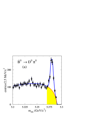
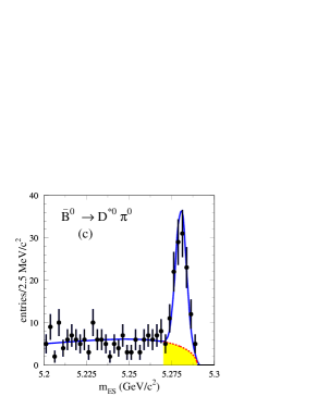
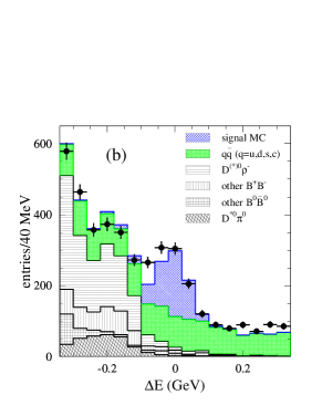
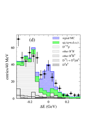
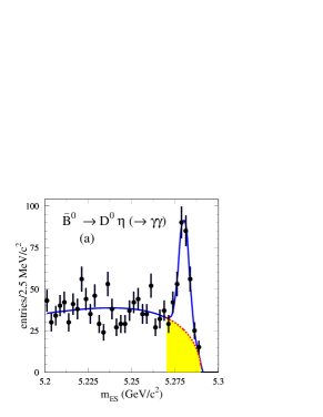
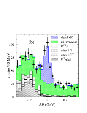
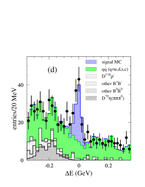
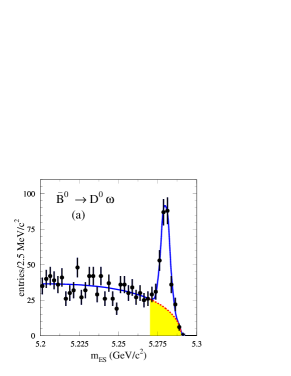
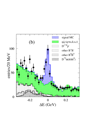
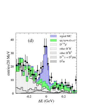
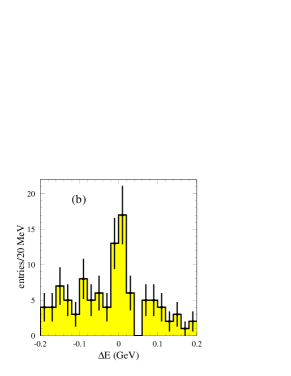
Figure 2: Distributions of $m_{\rm ES}$ and of $\Delta E$ for (a, b) candidate $\mbox{$\kern 1.79993pt\overline{\kern-1.79993ptB}{}^{0}$}\rightarrow\mbox{$D^{0}$}\mbox{$\pi^{0}$}$ events and (c, d) candidate $\mbox{$\kern 1.79993pt\overline{\kern-1.79993ptB}{}^{0}$}\rightarrow\mbox{$D^{*0}$}\mbox{$\pi^{0}$}$ events. The dots with error bars correspond to data. In the $m_{\rm ES}$ distribution, the ARGUS and Gaussian ML fits are superimposed. The number of signal candidates (${\cal N}_{cand}$), which includes peaking-background and cross-feed contributions, is the area of the Gaussian function in the signal region $5.270<\mbox{$m_{\rm ES}$}<5.290\,\mbox{${\rm GeV}/c^{2}$}$. The non-peaking background (${\cal N}_{\rm npb}$) is represented by the shaded region. The hatched histograms in the $\Delta E$ distributions represent the simulated events, and are shown separately for signal and the various backgrounds from $B\kern 1.79993pt\overline{\kern-1.79993ptB}{}$ and $q\overline{q}$ $(q=u,d,s,c)$ events.

Table 3: Total fractional cross-feed $({\cal F})$ expressed in percent (see text for definition) observed in the Monte Carlo simulation. The dominant sources that contribute are shown in decreasing order of importance.

$\kern 1.79993pt\overline{\kern-1.79993ptB}{}^{0}$ mode		${\cal F}_{\rm CF}(\%)$		Dominant sources
$D^{0}$$\pi^{0}$		3.6		$D^{*0}$$\pi^{0}$
$\mbox{$D^{*0}$}(\mbox{$D^{0}$}\mbox{$\pi^{0}$})\mbox{$\pi^{0}$}$		2.6		$\mbox{$D^{*0}$}(\mbox{$D^{0}$}\gamma)\mbox{$\pi^{0}$}$, $D^{0}$$\pi^{0}$
$\mbox{$D^{0}$}\eta(\gamma\gamma)$		5.4		$\mbox{$D^{*0}$}\eta$, $D^{0}$$\pi^{0}$, $D^{*0}$$\pi^{0}$
$\mbox{$D^{0}$}\eta(\mbox{\mbox{$\pi^{+}$}\mbox{$\pi^{-}$}\mbox{$\pi^{0}$}})$		2.2		$\mbox{$D^{*0}$}\eta$, $D^{0}$$\pi^{0}$, $\mbox{$D^{0}$}\omega$
$\mbox{$D^{*0}$}(\mbox{$D^{0}$}\mbox{$\pi^{0}$})\eta(\gamma\gamma)$		8.8		$\mbox{$D^{*0}$}(\mbox{$D^{0}$}\gamma)\eta$, $D^{*0}$$\pi^{0}$, $\mbox{$D^{0}$}\eta$
$\mbox{$D^{0}$}\omega$		2.5		$\mbox{$D^{*0}$}\omega$
$\mbox{$D^{*0}$}(\mbox{$D^{0}$}\mbox{$\pi^{0}$})\omega$		6.5		$\mbox{$D^{*0}$}(\mbox{$D^{0}$}\gamma)\omega$, $\mbox{$D^{0}$}\omega$,
				and $\mbox{$D^{0}$}\eta(\mbox{\mbox{$\pi^{+}$}\mbox{$\pi^{-}$}\mbox{$\pi^{0}$}})$

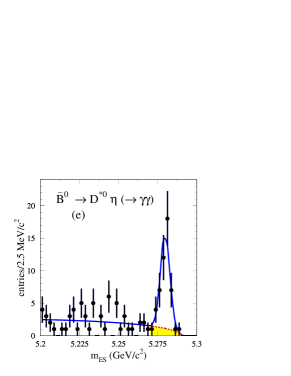
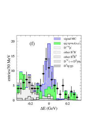
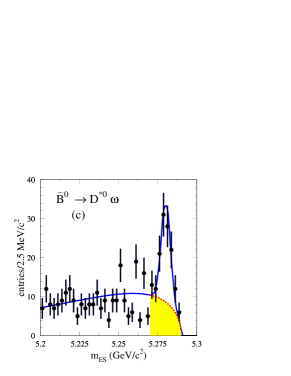
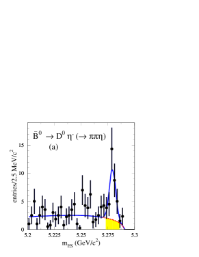
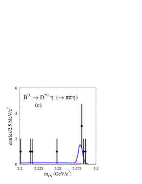
Figure 3: Distributions of $m_{\rm ES}$ and of $\Delta E$ for (a, b) candidate $\mbox{$\kern 1.79993pt\overline{\kern-1.79993ptB}{}^{0}$}\rightarrow\mbox{$D^{0}$}\eta$ ($\eta\rightarrow\gamma\gamma$) events, (c, d) candidate $\mbox{$\kern 1.79993pt\overline{\kern-1.79993ptB}{}^{0}$}\rightarrow\mbox{$D^{0}$}\eta$ ($\eta\rightarrow\mbox{\mbox{$\pi^{+}$}\mbox{$\pi^{-}$}\mbox{$\pi^{0}$}}$) events, and (e, f) candidate $\mbox{$\kern 1.79993pt\overline{\kern-1.79993ptB}{}^{0}$}\rightarrow\mbox{$D^{*0}$}\eta$ ($\eta\rightarrow\gamma\gamma$) events. The various contributions are shown as in Fig. 2.

Figure 4: Distributions of $m_{\rm ES}$ and of $\Delta E$ for (a, b) candidate $\mbox{$\kern 1.79993pt\overline{\kern-1.79993ptB}{}^{0}$}\rightarrow\mbox{$D^{0}$}\omega$ events and (c, d) candidate $\mbox{$\kern 1.79993pt\overline{\kern-1.79993ptB}{}^{0}$}\rightarrow\mbox{$D^{*0}$}\omega$ events. The various contributions are shown as in Fig. 2.

Figure 5: Distributions of $m_{\rm ES}$ and of $\Delta E$ of (a, b) candidate $\mbox{$\kern 1.79993pt\overline{\kern-1.79993ptB}{}^{0}$}\rightarrow\mbox{$D^{0}$}\eta^{\prime}$ events and (c, d) candidate $\mbox{$\kern 1.79993pt\overline{\kern-1.79993ptB}{}^{0}$}\rightarrow\mbox{$D^{*0}$}\eta^{\prime}$ events.

VI $\kern 1.79993pt\overline{\kern-1.79993ptB}{}^{0}$ candidates in the various color-suppressed decay modes

VI.1 $\mbox{$\kern 1.79993pt\overline{\kern-1.79993ptB}{}^{0}$}\rightarrow\mbox{$D^{0}$}\mbox{$\pi^{0}$}$

Figures 2(a) and 2(b) show the distributions in $m_{\rm ES}$ with $-90<\mbox{$\Delta E$}<100$ MeV and in $\Delta E$ with $5.270<\mbox{$m_{\rm ES}$}<5.290\,\mbox{${\rm GeV}/c^{2}$}$ for candidate $\mbox{$\kern 1.79993pt\overline{\kern-1.79993ptB}{}^{0}$}\rightarrow\mbox{$D^{0}$}\mbox{$\pi^{0}$}$ events. The solid line in Fig. 2(a) represents the ML fit to the sum of the ARGUS and Gaussian functions. In Fig. 2(b) the hatched histograms represent the simulated events for the signal and separately for the various backgrounds from $B\kern 1.79993pt\overline{\kern-1.79993ptB}{}$ and $q\overline{q}$ $(q=u,d,s,c)$ events.

Peaking backgrounds originate from color-allowed $\mbox{$B^{-}$}\rightarrow\mbox{$D^{0}$}\mbox{$\rho^{-}$}$ decays where the $\pi^{-}$ from the $\mbox{$\rho^{-}$}\rightarrow\mbox{$\pi^{-}$}\mbox{$\pi^{0}$}$ decay has very low momentum and is missed in the reconstruction of the $D^{0}$$\pi^{0}$ final state. This type of background populates the $\Delta E$ plot in the region that is at least one pion mass below the signal region. It produces a peak in the $m_{\rm ES}$ distribution in and slightly below the signal region. Resolution effects in $\Delta E$ will cause some events to migrate from below the signal region into the signal region and thus contribute to the signal peak in the $m_{\rm ES}$ distribution.

A veto on the color-allowed $\mbox{$B^{-}$}\rightarrow\mbox{$D^{0}$}\mbox{$\rho^{-}$}$ decays is applied as part of the selection of the $\kern 1.79993pt\overline{\kern-1.79993ptB}{}^{0}$ candidates. A $\kern 1.79993pt\overline{\kern-1.79993ptB}{}^{0}$ candidate is rejected if it can be reconstructed as a $\mbox{$B^{-}$}\rightarrow\mbox{$D^{0}$}\mbox{$\rho^{-}$}$ candidate with the following properties:

• It uses the same $D^{0}$ and $\pi^{0}$ as the $\kern 1.79993pt\overline{\kern-1.79993ptB}{}^{0}$ candidate and the $\rho^{-}$ meson is selected as described in Sec. IV.2.1.

• The $m_{\rm ES}$ is within 9 ${\rm MeV}/c^{2}$ of the nominal $B^{-}$ mass and $|\mbox{$\Delta E$}|<100$ MeV.

According to the Monte Carlo simulation, this veto removes only a few percent of signal events, while it rejects about 70% of $D^{0}$$\rho^{-}$ events and 60% of $D^{*0}$$\rho^{-}$ events. This background reduction occurs nearly entirely in the $\Delta E$ region below approximately one pion mass and the veto is less effective in the signal region, where only a few percents of the background events are rejected.

The veto is nevertheless very useful because it decreases the $\Delta E$ distribution in the region just below the signal region, thereby reducing the likelihood that the finite energy resolution will shift events from the negative $\Delta E$ region into the signal region. The precise determination of the resolution here is related to the resolution of the EMC for relatively energetic $\pi^{0}$ mesons. Removing a large fraction of these background events at and below the lower signal region limit reduces substantially this uncertainty. Even after the veto is applied, as it can be seen in Fig. 2(b), the shape of the $\Delta E$ distribution for this background changes abruptly at about minus one pion mass and that below this limit the magnitude of the $\mbox{$B^{-}$}\rightarrow\mbox{$D^{(*)0}$}\mbox{$\rho^{-}$}$ background can still not be neglected.

The yield of the fitted candidate $D^{0}$$\pi^{0}$ events and the numbers for the various background contributions to this decay mode are listed in Table 2.

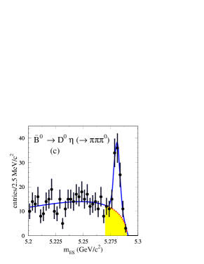
VI.2 $\mbox{$\kern 1.79993pt\overline{\kern-1.79993ptB}{}^{0}$}\rightarrow\mbox{$D^{*0}$}\mbox{$\pi^{0}$}$

Figures 2(c) and 2(d) show the distributions in $m_{\rm ES}$ with $-90<\mbox{$\Delta E$}<100\,\mbox{\rm MeV}$ and in $\Delta E$ with $5.270<\mbox{$m_{\rm ES}$}<5.290\,\mbox{${\rm GeV}/c^{2}$}$ for the candidate $\mbox{$\kern 1.79993pt\overline{\kern-1.79993ptB}{}^{0}$}\rightarrow\mbox{$D^{*0}$}\mbox{$\pi^{0}$}$ events.

The $D^{*0}$$\pi^{0}$ candidates are contaminated by color-allowed $\mbox{$B^{-}$}\rightarrow\mbox{$D^{(*)0}$}\mbox{$\rho^{-}$}$ decays. Events from $\mbox{$B^{-}$}\rightarrow\mbox{$D^{(*)0}$}\mbox{$\rho^{-}$}$ can enter the signal region when the soft $\pi^{-}$ from the $\rho^{-}$ decay is missed. In the case of $D^{0}$$\rho^{-}$ events an unrelated $\pi^{0}$ is used to reconstruct the $D^{*0}$ meson. For this mode we veto both $\mbox{$B^{-}$}\rightarrow\mbox{$D^{0}$}\mbox{$\rho^{-}$}$ and $D^{*0}$$\rho^{-}$ decays. The criteria used to veto $\kern 1.79993pt\overline{\kern-1.79993ptB}{}^{0}$ candidates are the same as for the veto described in the $D^{0}$$\pi^{0}$ subsection except that for $D^{*0}$$\pi^{0}$ the $\kern 1.79993pt\overline{\kern-1.79993ptB}{}^{0}$ candidate is rejected if there is a $\mbox{$B^{-}$}\rightarrow\mbox{$D^{(*)0}$}\mbox{$\rho^{-}$}$ candidate that uses the same $D^{(*)0}$ and $\pi^{0}$ mesons as the $\kern 1.79993pt\overline{\kern-1.79993ptB}{}^{0}$ candidate.

According to the Monte Carlo simulation this veto rejects about 65% of $D^{0}$$\rho^{-}$ events and 70% of $D^{*0}$$\rho^{-}$ events and the signal efficiency is close to 80%. The veto is relatively less effective in the signal region of the $\Delta E$ distribution, where 60% of $D^{0}$$\rho^{-}$ events and 40% of $D^{*0}$$\rho^{-}$ events are rejected. As in the $D^{0}$$\pi^{0}$ case discussed above, the veto reduces the systematic uncertainty related to the background estimate.

The yield of the fitted candidate $D^{*0}$$\pi^{0}$ events and the numbers for the various background contributions to this decay mode are listed in Table 2.

VI.3 $\mbox{$\kern 1.79993pt\overline{\kern-1.79993ptB}{}^{0}$}\rightarrow\mbox{$D^{0}$}\eta$

Figures 3(a) and 3(b) show the distributions in $m_{\rm ES}$ with $|\mbox{$\Delta E$}|<89\,\mbox{\rm MeV}$ (3 times the $\Delta E$ resolution measured in the Monte Carlo simulation) and in $\Delta E$ with $5.270<\mbox{$m_{\rm ES}$}<5.290\,\mbox{${\rm GeV}/c^{2}$}$ for candidate $\mbox{$\kern 1.79993pt\overline{\kern-1.79993ptB}{}^{0}$}\rightarrow\mbox{$D^{0}$}\eta$ events, where the $\eta$ meson is reconstructed in the $\gamma\gamma$ decay channel. Figures 3(c) and 3(d) show the same distributions when the $\eta$ meson is reconstructed in the $\pi^{+}$$\pi^{-}$$\pi^{0}$ decay channel. Here the selection $|\mbox{$\Delta E$}|<54\,\mbox{\rm MeV}$ is applied (again 3 times the $\Delta E$ resolution) in the $m_{\rm ES}$ distribution.

In the $\eta\rightarrow\gamma\gamma$ case, the contribution to the peaking background from $\mbox{$B^{-}$}\rightarrow\mbox{$D^{(*)0}$}\mbox{$\rho^{-}$}$ decays is dominant. It corresponds to 80% of the peaking background. In this case a photon from the fast $\pi^{0}$ in the $\rho^{-}$ decay is combined with another photon to form an $\eta$ candidate. This background is sufficiently suppressed by the $\pi^{0}$ veto described in Sec. IV.2.2 so that no additional requirements are imposed.

According to the Monte Carlo simulation, the peaking background is negligible in the $\pi^{+}$$\pi^{-}$$\pi^{0}$ decay channel. The Monte Carlo simulation includes processes such as $D^{(\ast)}\pi^{-}\pi^{-}\pi^{+}\mbox{$\pi^{0}$}$ that may fake a $\mbox{$\kern 1.79993pt\overline{\kern-1.79993ptB}{}^{0}$}\rightarrow\mbox{$D^{0}$}\eta(\rightarrow\mbox{\mbox{$\pi^{+}$}\mbox{$\pi^{-}$}\mbox{$\pi^{0}$}})$ signal if one charged $\pi$ is lost in the reconstruction of the $\kern 1.79993pt\overline{\kern-1.79993ptB}{}^{0}$ meson. The branching fractions for these modes have been measured recently by the CLEO collaboration ref:cleoDrhoprime . Because these backgrounds are shifted in $\Delta E$ by more than the mass of the missing $\pi$ and because the $\eta$ mass selection is quite tight, the Monte Carlo simulation indicates that no events originating from such modes are selected within the signal region. We checked the effect of widening the signal region to $|\mbox{$\Delta E$}|<110\,\mbox{\rm MeV}$. Due to resolution effects more background events in the $\Delta E$ sideband region migrate into the wider $\Delta E$ signal region; we observe that in that latter case about 10% of the total $B\kern 1.79993pt\overline{\kern-1.79993ptB}{}$ background is generated by ${\rm D}^{(\ast)}\eta(\rightarrow\mbox{\mbox{$\pi^{+}$}\mbox{$\pi^{-}$}\mbox{$\pi^{0}$}})\pi^{-}$ decays.

The yields of the fitted candidate $\mbox{$D^{0}$}\eta$ events for the $\eta\rightarrow\gamma\gamma$ and $\pi^{+}$$\pi^{-}$$\pi^{0}$ decay modes and the numbers for the various background contributions to these decay modes are listed in Table 2.

VI.4 $\mbox{$\kern 1.79993pt\overline{\kern-1.79993ptB}{}^{0}$}\rightarrow\mbox{$D^{*0}$}\eta$

Figures 3(e) and 3(f) show the distributions in $m_{\rm ES}$ with $|\mbox{$\Delta E$}|<92\,\mbox{\rm MeV}$ (3 times the $\Delta E$ resolution measured in the Monte Carlo simulation) and in $\Delta E$ with $5.270<\mbox{$m_{\rm ES}$}<5.290\,\mbox{${\rm GeV}/c^{2}$}$ for candidate $\mbox{$\kern 1.79993pt\overline{\kern-1.79993ptB}{}^{0}$}\rightarrow\mbox{$D^{*0}$}\eta$ events in which the $\eta$ meson is reconstructed in the $\gamma\gamma$ channel.

According to the Monte Carlo simulation, the peaking background is negligible. The yield of the fitted candidate $\mbox{$D^{*0}$}\eta$ events and the numbers for the various background contributions to this decay mode are listed in Table 2. The statistical significance of the signal is $5.5$.

VI.5 $\mbox{$\kern 1.79993pt\overline{\kern-1.79993ptB}{}^{0}$}\rightarrow\mbox{$D^{0}$}\omega$

Figures 4(a) and 4(b) show the distributions in $m_{\rm ES}$ with $|\mbox{$\Delta E$}|<61\,\mbox{\rm MeV}$ (3 times the $\Delta E$ resolution measured in the Monte Carlo simulation), and in $\Delta E$ with $5.270<\mbox{$m_{\rm ES}$}<5.290\,\mbox{${\rm GeV}/c^{2}$}$ for the candidate $\mbox{$\kern 1.79993pt\overline{\kern-1.79993ptB}{}^{0}$}\rightarrow\mbox{$D^{0}$}\omega$ events. Due to the tight $\omega$ mass selection and the angular selections, the peaking background is small.

For the peaking-background determination, we have included possible contributions from $D^{(\ast)}\pi^{-}\pi^{-}\pi^{+}\mbox{$\pi^{0}$}$ decays. CLEO ref:cleoDrhoprime reports the observation of these processes, gives branching fractions for $D^{\ast}\pi^{-}\pi^{-}\pi^{+}\mbox{$\pi^{0}$}$ and $D^{(\ast)}\omega\pi^{-}$, and provides evidence for $D^{(\ast)}\rho^{\prime-}(\rightarrow\omega\pi^{-})$. These measurements have been performed for both charged and neutral $B$ decays. If the additional $\pi^{-}$ from the $\rho^{\prime-}$ decay is missed, these decays can fake $\mbox{$\kern 1.79993pt\overline{\kern-1.79993ptB}{}^{0}$}\rightarrow\mbox{$D^{0}$}\omega$ events. But Monte Carlo simulation indicates that the $\Delta E$ distribution for this background is shifted by more than the mass of the missing pion and rarely falls in the signal region. We estimate from the Monte Carlo simulation that about 11% of the total $B^{0}$$\kern 1.79993pt\overline{\kern-1.79993ptB}{}^{0}$ background in the signal region originates from ${\rm D}^{(\ast)+}\omega\pi^{-}$ modes; similarly, 13% of the total $B^{+}$$B^{-}$ background is from $\mbox{$D^{(*)0}$}\omega\pi^{-}$ decays. These fractions remain the same if the $\Delta E$ signal range is extended to $|\mbox{$\Delta E$}|<100\,\mbox{\rm MeV}$, thus indicating that the $D^{(\ast)}\pi^{-}\pi^{-}\pi^{+}\mbox{$\pi^{0}$}$ background is randomly distributed in $\Delta E$ over the signal region. We also find that $D^{(\ast)}\rho$ events contribute about 5% of the total $B\kern 1.79993pt\overline{\kern-1.79993ptB}{}$ background.

The yield of the fitted candidate $\mbox{$D^{0}$}\omega$ events and the numbers for the various background contributions to this decay mode are listed in Table 2.

VI.6 $\mbox{$\kern 1.79993pt\overline{\kern-1.79993ptB}{}^{0}$}\rightarrow\mbox{$D^{*0}$}\omega$

Figures 4(c) and 4(d) show the distributions in $m_{\rm ES}$ with $|\mbox{$\Delta E$}|<61\,\mbox{\rm MeV}$ (3 times the $\Delta E$ resolution measured in the Monte Carlo simulation) and in $\Delta E$ with $5.270<\mbox{$m_{\rm ES}$}<5.290\,\mbox{${\rm GeV}/c^{2}$}$ for candidate $\mbox{$\kern 1.79993pt\overline{\kern-1.79993ptB}{}^{0}$}\rightarrow\mbox{$D^{*0}$}\omega$ events.

As for the $\mbox{$D^{0}$}\omega$ analysis, when determining the peaking background, the effect of $D^{(\ast)}\mbox{$\pi^{-}$}\mbox{$\pi^{-}$}\mbox{$\pi^{+}$}\mbox{$\pi^{0}$}$ decays has been evaluated. In this case the mode $\mbox{$B^{-}$}\rightarrow\mbox{$D^{0}$}\omega\pi^{-}$ may contaminate the signal when the $\pi^{-}$ is replaced by a $\pi^{0}$ to fake a $D^{*0}$ meson. However, the kinematics of the soft $\pi^{0}$ in the $D^{*0}$ decay for the $\mbox{$D^{*0}$}\omega$ signal is very different from those of the $\pi^{-}$ where the momentum can be large. In addition the relatively small branching fraction for the $\mbox{$D^{0}$}\omega\pi^{-}$ decays implies that the contribution from this background in the signal region is not expected to be important. We estimate from the Monte Carlo simulation that 16% of the total $B^{+}$$B^{-}$ background in the signal region originates from $\mbox{$D^{(*)0}$}\omega\pi^{-}$ modes. No contribution to the $B^{0}$$\kern 1.79993pt\overline{\kern-1.79993ptB}{}^{0}$ background from the ${\rm D}^{(\ast)+}\omega\pi^{-}$ decays has been found. The fractions remain the same when the $\Delta E$ range of the signal region is extended to $|\mbox{$\Delta E$}|<100\,\mbox{\rm MeV}$. Again, this confirms that this type of background is uniformly distributed in $\Delta E$ over the signal region and rules out any significant contribution to the peaking background from these decays. We also find that $D^{(\ast)}\rho$ events contribute about 5% of the total $B\kern 1.79993pt\overline{\kern-1.79993ptB}{}$ background. The peaking background for this decay mode is found to be negligible.

The yield of the fitted candidate $\mbox{$D^{*0}$}\omega$ events and the numbers for the various background contributions to this decay mode are listed in Table 2. The statistical significance of the signal is $6.1$.

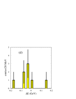
VI.7 $\mbox{$\kern 1.79993pt\overline{\kern-1.79993ptB}{}^{0}$}\rightarrow\mbox{$D^{0}$}\eta^{\prime}$

Figure 5(a) shows the $m_{\rm ES}$ distribution for $\mbox{$D^{0}$}\rightarrow\mbox{$\mbox{$K^{-}$}\mbox{$\pi^{+}$}$}$ with $|\mbox{$\Delta E$}|<60\,\mbox{\rm MeV}$ and for $\mbox{$D^{0}$}\rightarrow\mbox{$\mbox{$K^{-}$}\mbox{$\pi^{+}$}\mbox{$\pi^{0}$}$}$ and $K^{-}$$\pi^{+}$$\pi^{+}$$\pi^{-}$ with $|\mbox{$\Delta E$}|<40\,\mbox{\rm MeV}$. Figure 5(b) shows the $\Delta E$ distribution with $5.273<\mbox{$m_{\rm ES}$}<5.286\,\mbox{${\rm GeV}/c^{2}$}$. According to the Monte Carlo simulation, the peaking background in this channel is negligible. As reported in Table 2, the fit yields $\mbox{${\cal N}_{\rm cand}$}=26.6\pm 6.0$ candidate $D^{0}$$\eta^{\prime}$ events and $\mbox{${\cal N}_{\rm npb}$}=10.4\pm 1.1$ combinatorial-background events. The statistical significance of the signal, calculated from Poisson statistics, is $6.3$.

VI.8 $\mbox{$\kern 1.79993pt\overline{\kern-1.79993ptB}{}^{0}$}\rightarrow\mbox{$D^{*0}$}\eta^{\prime}$

Figure 5(c) shows the $m_{\rm ES}$ distribution for $\mbox{$D^{0}$}\rightarrow\mbox{$\mbox{$K^{-}$}\mbox{$\pi^{+}$}$}$ with $|\mbox{$\Delta E$}|<60\,\mbox{\rm MeV}$ and for $\mbox{$D^{0}$}\rightarrow\mbox{$\mbox{$K^{-}$}\mbox{$\pi^{+}$}\mbox{$\pi^{0}$}$}$ and $K^{-}$$\pi^{+}$$\pi^{+}$$\pi^{-}$ with $|\mbox{$\Delta E$}|<40\,\mbox{\rm MeV}$. Figure 5(d) shows the $\Delta E$ distribution with $5.273<\mbox{$m_{\rm ES}$}<5.286\,\mbox{${\rm GeV}/c^{2}$}$. According to the Monte Carlo simulation the peaking background is negligible. As reported in Table 2, the fit yields $\mbox{${\cal N}_{\rm cand}$}=4.0\pm 2.2$ candidate $D^{*0}$$\eta^{\prime}$ events and $\mbox{${\cal N}_{\rm npb}$}=0.5\pm 0.3$ combinatorial-background events. The statistical significance of the signal, calculated from Poisson statistics, is only $3.0$.

Table 4: Acceptance (${\cal A}$), corrected acceptance (${\cal A}_{\rm{corr}}$) obtained after differences between Monte Carlo simulation of detector response and data are taken into account, and overall efficiency $({\cal E})$ that includes branching fractions from secondary decays. The uncertainties associated with these numbers are discussed in Sec. VIII.

$\kern 1.79993pt\overline{\kern-1.79993ptB}{}^{0}$ mode		${\cal A}$ (%)		${\cal A}_{\rm{corr}}$ (%)		${\cal E}(\%)$
(decay channel)
$D^{0}$$\pi^{0}$		9.1		7.9		1.87
$D^{*0}$$\pi^{0}$		2.7		2.3		0.34
$\mbox{$D^{0}$}\eta(\rightarrow\gamma\gamma)$		9.7		8.6		0.82
$\mbox{$D^{0}$}\eta(\rightarrow\mbox{\mbox{$\pi^{+}$}\mbox{$\pi^{-}$}\mbox{$\pi^{0}$}})$		6.5		5.6		0.30
$\mbox{$D^{*0}$}\eta(\rightarrow\gamma\gamma)$		3.3		2.8		0.17
$\mbox{$D^{0}$}\omega$		4.2		3.5		0.75
$\mbox{$D^{*0}$}\omega$		1.7		1.4		0.19
$\mbox{$D^{0}$}\eta^{\prime}$		5.0		4.2		0.18
$\mbox{$D^{*0}$}\eta^{\prime}$		1.6		1.4		0.035

Table 5: Values of ${\cal A}_{\rm{corr}}$, ${\cal B}(\mbox{$D^{0}$})$ (the branching fraction of the various $D^{0}$ decay modes ref:PDG ), ${\cal B}_{\rm sec}$ (the product of the branching fractions associated with the secondary decays of the $\eta\rightarrow\gamma\gamma$ and the $D^{0}$), and ${\cal E}$ for the $\mbox{$B^{0}$}\rightarrow\mbox{$D^{0}$}\eta(\gamma\gamma)$ decay mode. The branching fraction for the $\eta\rightarrow\gamma\gamma$ is taken to be 39.4% ref:PDG . The uncertainties associated with these numbers are discussed in Sec. VIII.

$D^{0}$ decay		$\mbox{${\cal A}_{\rm{corr}}$}(\%)$		${\cal B}(\mbox{$D^{0}$})(\%)$		$\mbox{${\cal B}_{\rm sec}$}(\%)$		${\cal E}(\%)$
$K^{-}$$\pi^{+}$		19.5		3.8		1.5		0.29
$K^{-}$$\pi^{+}$$\pi^{0}$		6.0		13.1		5.1		0.31
$K^{-}$$\pi^{+}$$\pi^{+}$$\pi^{-}$		7.4		7.5		2.9		0.22
all		8.6		-		9.5		0.82

VII Branching Fractions

The acceptance ${\cal A}$ for signal events is estimated from signal Monte Carlo as

$${\cal A}=\frac{{S}_{\rm MC}}{N_{\rm gen}}\mbox{.}$$ (19)

Where ${S}_{\rm MC}$ is the number of events in the signal region that pass the selection criteria and $N_{\rm gen}$ is the number of generated signal Monte Carlo events.

The selection efficiencies for each mode are obtained from detailed Monte Carlo studies in which the detector response is simulated using the GEANT4 ref:GEANT program. The efficiencies of tracking, detection and reconstruction in the EMC, vertex fitting, and particle identification have been measured in control sets of data and compared with their Monte Carlo simulation. We correct the acceptance for differences between data and Monte Carlo simulation of these effects by using precise correction factors that are applied to each track (for track reconstruction efficiency), to each photon, $\pi^{0}$, $\eta(\gamma\gamma)$ (for neutral cluster detection efficiency and energy resolution), to each kaon candidate (for particle identification efficiency), and to each vertex-fit (for vertex-fit efficiency). Most of these corrections depend upon the polar angle and momenta of the tracks and neutral clusters and some also depend on the running conditions.

Tracking efficiencies are determined by identifying tracks in the SVT and measuring the fraction of tracks that are reconstructed in the DCH. The $\gamma$ and $\pi^{0}$ efficiencies are measured by comparing the ratio of the number of events $N(\tau^{+}\to\overline{\nu}_{\tau}h^{+}\mbox{$\pi^{0}$})$ and $N(\tau^{+}\to\overline{\nu}_{\tau}h^{+}\mbox{$\pi^{0}$}\mbox{$\pi^{0}$})$ to the known branching fractions ref:cleotau . The kaon identification efficiency is estimated from a sample of $\mbox{$D^{*+}$}\rightarrow\mbox{$D^{0}$}\mbox{$\pi^{+}$}$, $\mbox{$D^{0}$}\rightarrow\mbox{$\mbox{$K^{-}$}\mbox{$\pi^{+}$}$}$ decays that are identified kinematically. Based on a similar selection, a sample of $\mbox{$\kern 1.79993pt\overline{\kern-1.79993ptB}{}^{0}$}\rightarrow\mbox{$D^{*+}$}\mbox{$\pi^{-}$}$, $\mbox{$D^{*+}$}\rightarrow\mbox{$D^{0}$}\mbox{$\pi^{+}$}$, $\mbox{$D^{0}$}\rightarrow\mbox{$\mbox{$K^{-}$}\mbox{$\pi^{+}$}$}$, $K^{-}$$\pi^{+}$$\pi^{0}$, or $K^{-}$$\pi^{+}$$\pi^{+}$$\pi^{-}$ decays is used to determine the vertex-fit efficiency corrections.

The acceptances ${\cal A}$ obtained with Eq. (19) and the corrected acceptances ${\cal A}_{\rm{corr}}$ are listed in Table 4. The last column in Table 4 lists the values of the overall efficiency ${\cal E}$ defined as

$${\cal E}=\mbox{${\cal A}_{\rm{corr}}$}\times\mbox{${\cal B}_{\rm sec}$}{\rm,}$$ (20)

where

$$\begin{split}{\mbox{${\cal B}_{\rm sec}$}}=\mbox{${\cal B}$}(\mbox{$D^{*0}$}\rightarrow\mbox{$D^{0}$}\mbox{$\pi^{0}$})\times\mbox{${\cal B}$}(\mbox{$\pi^{0}$}\rightarrow\gamma\gamma)\times\ \\ \mbox{${\cal B}$}(\mbox{$h^{0}$}\rightarrow Y)\times\sum_{X}{\mbox{${\cal B}$}(\mbox{$D^{0}$}\rightarrow X)}\end{split}$$ (21)

is the product of the branching fractions associated with the secondary decays of the $D^{*0}$, $h^{0}$, and $D^{0}$ (with $X=\mbox{$\mbox{$K^{-}$}\mbox{$\pi^{+}$}$}$, $K^{-}$$\pi^{+}$$\pi^{0}$, or $K^{-}$$\pi^{+}$$\pi^{+}$$\pi^{-}$). The $\mbox{${\cal B}$}(\mbox{$D^{*0}$}\rightarrow\mbox{$D^{0}$}\mbox{$\pi^{0}$})\times\mbox{${\cal B}$}(\mbox{$\pi^{0}$}\rightarrow\gamma\gamma)$ factor is only present for the $\mbox{$\kern 1.79993pt\overline{\kern-1.79993ptB}{}^{0}$}\rightarrow\mbox{$D^{*0}$}\mbox{$h^{0}$}$ final states. Note that the overall efficiency ${\cal E}$ for the $\mbox{$D^{(*)0}$}\eta^{\prime}$ decays is reduced with respect to the other $\kern 1.79993pt\overline{\kern-1.79993ptB}{}^{0}$ modes by the relatively small values of ${\cal B}_{\rm sec}$.

In Table 5 we display, as an example, the contributions of the three $D^{0}$ final states in the decay mode $\mbox{$\kern 1.79993pt\overline{\kern-1.79993ptB}{}^{0}$}\rightarrow\mbox{$D^{0}$}\eta(\gamma\gamma)$. There are variations between the acceptance and branching fraction for the three $D^{0}$ decay modes leading to similar values of ${\cal E}$ for the three modes. A similar conclusion holds for other $\mbox{$\kern 1.79993pt\overline{\kern-1.79993ptB}{}^{0}$}\rightarrow\mbox{$D^{(*)0}$}\mbox{$h^{0}$}$ final states.

To obtain branching fractions, the number of background subtracted signal events, $S$, is divided by the number of $B\kern 1.79993pt\overline{\kern-1.79993ptB}{}$ events in the data sample, $N(\mbox{$B\kern 1.79993pt\overline{\kern-1.79993ptB}{}$})$, and the overall efficiency, ${\cal E}$:

$${\mbox{${\cal B}$}}(\mbox{$\kern 1.79993pt\overline{\kern-1.79993ptB}{}^{0}$}\rightarrow\mbox{$D^{(*)0}$}\mbox{$h^{0}$})=\frac{S}{N(\mbox{$B\kern 1.79993pt\overline{\kern-1.79993ptB}{}$})\times{\cal E}}{\rm.}$$ (22)

These branching fraction calculations assume equal production of $B^{0}$$\kern 1.79993pt\overline{\kern-1.79993ptB}{}^{0}$ and $B^{+}B^{-}$ pairs at the $\mathchar 28935\relax{(4S)}$ resonance.

Table 6: Systematic uncertainties of the measured branching fractions in percent. The symbol “-” indicates that the systematic uncertainty is negligible.

Category		$D^{0}$$\pi^{0}$		$D^{*0}$$\pi^{0}$		$\mbox{$D^{0}$}\eta(\gamma\gamma)$		$\mbox{$D^{0}$}\eta(\mbox{\mbox{$\pi^{+}$}\mbox{$\pi^{-}$}\mbox{$\pi^{0}$}})$		$\mbox{$D^{*0}$}\eta$		$\mbox{$D^{0}$}\omega$		$\mbox{$D^{*0}$}\omega$		$\mbox{$D^{0}$}\eta^{\prime}$		$\mbox{$D^{*0}$}\eta^{\prime}$
Tracking		2.1		2.1		2.0		3.6		2.0		3.6		3.6		3.6		3.6
Vertex-fit		1.4		1.4		1.4		2.5		1.4		2.5		2.5		1.4		1.4
Kaon identification		2.5		2.5		2.5		2.5		2.5		2.5		2.5		2.5		2.5
$\gamma$, $\pi^{0}$, and $\eta$ detection		5.2		8.1		3.7		6.0		6.8		5.9		9.1		3.5		6.5
Cross-feed		1.0		0.7		1.4		0.5		2.4		0.6		1.7		-		-
$\Delta E$ resolution		1.7		1.9		3.0		4.4		3.5		5.7		3.3		-		-
$m_{\rm ES}$ fit		0.3		3.2		4.5		4.8		8.4		3.0		10.3		2.3		2.3
Peaking background		3.3		6.3		3.2		2.0		0.5		3.4		4.0		-		-
Event selection		6.8		9.4		6.1		8.9		7.6		6.8		11.9		7.9		7.9
${\cal B}(\mbox{$D^{(*)0}$})$ and ${\cal B}($$h^{0}$$)$		4.6		6.6		4.4		4.6		6.3		4.3		6.4		5.6		7.3
Number of $B\kern 1.79993pt\overline{\kern-1.79993ptB}{}$ pairs		1.1		1.1		1.1		1.1		1.1		1.1		1.1		1.1		1.1
Monte Carlo statistics		0.7		2.2		1.3		1.6		2.0		1.6		2.9		1.6		1.6
Total (%)		11.1		16.4		11.2		14.5		15.8		13.5		20.8		11.7		13.7

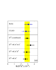
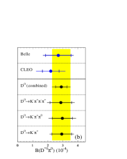
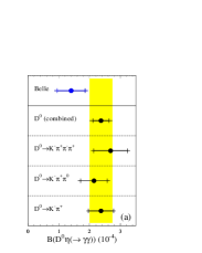
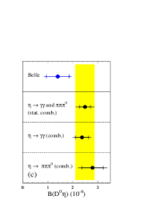
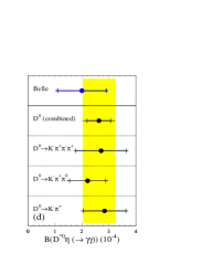
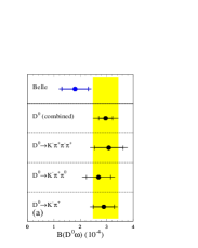
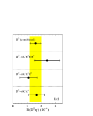
Figure 6: Measured branching fractions for each of the three $D^{0}$ decay modes and for the combination of the three for (a) $\mbox{$\kern 1.79993pt\overline{\kern-1.79993ptB}{}^{0}$}\rightarrow\mbox{$D^{0}$}\mbox{$\pi^{0}$}$ and (b) $\mbox{$\kern 1.79993pt\overline{\kern-1.79993ptB}{}^{0}$}\rightarrow\mbox{$D^{*0}$}\mbox{$\pi^{0}$}$. The shaded bands represent the results from the present investigation. The length of the error bars is equal to the sum in quadrature of the statistical and the systematic uncertainty; the statistical contribution is superimposed on the error bar. The CLEO ref:CLEO and Belle ref:Belle results are also shown.

VIII Systematic Uncertainties

Systematic uncertainties are associated with the acceptance corrections discussed in Sec. VII. The uncertainties from the tracking-efficiency corrections are 0.8% per charged track. To take into account uncertainties caused by the vertex reconstruction, we assign a systematic uncertainty equal to 1.1% per two-track vertex and 2.2% per four-track vertex. For particle identification the uncertainty is 2.5% per $K^{\pm}$ track. The uncertainties from the requirement that all the $\pi^{\pm}$ daughters must fail the tight kaon criterion are negligible. Uncertainties in the acceptances for photon detection account for imperfect simulation of photon-energy and position resolution, thus affecting $\pi^{0}$ and $\eta$ reconstruction efficiencies and the $\Delta E$ resolution. For the detection of isolated $\pi^{0}$ and $\eta(\gamma\gamma)$ mesons uncertainties of 5% and 2.5% are used. These uncertainties are summed in quadrature, together with other corrections that depend upon the energy of each $\gamma$ used to reconstruct the mesons.

We consider systematic uncertainties from other sources. For the cross-feed fractions an uncertainty equal to 25% of the estimated fraction accounts for uncertainties in the branching fractions reported in this study and used in the cross-feed determination. This value is chosen conservatively; it corresponds to the branching fraction measurement with the largest uncertainty reported in this paper (see Table 8).

The effect of the specific $\Delta E$ range used to define the signal region and based on the resolution measured from the Monte Carlo simulation has been estimated by varying the limits of the range by $\pm\ 0.5\,\sigma$. The observed variations in the branching fraction are used to determine the systematic uncertainty from this source. In the case of the $D^{(*)0}$$\pi^{0}$ modes, we vary the lower limit on the signal region definition ($-90<\mbox{$\Delta E$}<100\,\mbox{\rm MeV}$) between $-110$ and $-60$ MeV. Therefore, this procedure also accounts for uncertainties in the peaking-background estimates that are caused by the systematic uncertainty of the energy resolution that originates from the EMC.

To evaluate the systematic uncertainty associated with using the $m_{\rm ES}$ resolution taken from Monte Carlo in the fit to data, we also let it vary freely in that fit and half of the variation in the yields is taken as the systematic error. We also investigate the uncertainties in the combinatorial background due to setting the value of the ARGUS shape parameter $\xi$ to the value obtained in the fit to the data $m_{\rm ES}$ distribution in the upper $\Delta E$ sideband $+\ 6\,\sigma<\mbox{$\Delta E$}<350\,\mbox{\rm MeV}$. For the $\mbox{$D^{(*)0}$}\eta^{\prime}$ analyses, the value of $\xi$ is obtained from the $\Delta E$ sidebands (see Sec. IV.4.3). We therefore vary the value of $\xi$ by one standard deviation of the statistical error. In each case we take half the variation observed as the systematic uncertainty. Finally, the sum of the systematic errors from the ARGUS shape parameter and the fixed Gaussian width is taken as the systematic error for the $m_{\rm ES}$ fitting procedure.

Systematic uncertainties in the peaking background arise from imprecision in branching fractions and from statistical uncertainties in the number of peaking-background events obtained from the procedure described in Sec. V.1. For the $D^{(*)0}$$\pi^{0}$ modes the systematic uncertainty associated with the veto of the $\mbox{$B^{-}$}\rightarrow\mbox{$D^{(*)0}$}\mbox{$\rho^{-}$}$ background has been studied and is part of the systematic uncertainty of the background estimate. For these $D^{(*)0}$$\pi^{0}$ decay modes, we remove the veto on the $\mbox{$B^{-}$}\rightarrow\mbox{$D^{(*)0}$}\mbox{$\rho^{-}$}$ background and we include in the uncertainties half of the relative variation of the branching fraction. Finally, we have explained in Sec. V.1 how the systematic uncertainty related to the fitting method used in the calculation of the number of peaking-background events is estimated. The variation of the branching fraction due to the latter effect is small or negligible (4% at most) but is included in the systematic uncertainty from peaking background.

Figure 7: Measured branching fractions for each of the three $D^{0}$ decay modes and for the combination of the three for (a) $\mbox{$\kern 1.79993pt\overline{\kern-1.79993ptB}{}^{0}$}\rightarrow\mbox{$D^{0}$}\eta(\rightarrow\gamma\gamma)$, (b) $\mbox{$\kern 1.79993pt\overline{\kern-1.79993ptB}{}^{0}$}\rightarrow\mbox{$D^{0}$}\eta(\rightarrow\mbox{\mbox{$\pi^{+}$}\mbox{$\pi^{-}$}\mbox{$\pi^{0}$}})$, (c) each of the $\mbox{$\kern 1.79993pt\overline{\kern-1.79993ptB}{}^{0}$}\rightarrow\mbox{$D^{0}$}\eta$ modes and their combination, and (d) $\mbox{$\kern 1.79993pt\overline{\kern-1.79993ptB}{}^{0}$}\rightarrow\mbox{$D^{*0}$}\eta$. The branching fraction for the $\mbox{$D^{0}$}\eta$ channel is obtained as the average of the branching fraction of each of the two $\eta$ decay modes, weighted by the statistical uncertainties of these decays. The computation of the systematic uncertainty includes both the correlated and uncorrelated uncertainties of these two modes. The Belle ref:Belle results are also shown. The error bars are as in Fig. 6.

Figure 8: Measured branching fractions for each of the three $D^{0}$ decay modes and for the combination of the three for (a) $\mbox{$\kern 1.79993pt\overline{\kern-1.79993ptB}{}^{0}$}\rightarrow\mbox{$D^{0}$}\omega$, (b) $\mbox{$\kern 1.79993pt\overline{\kern-1.79993ptB}{}^{0}$}\rightarrow\mbox{$D^{*0}$}\omega$, and (c) $\mbox{$\kern 1.79993pt\overline{\kern-1.79993ptB}{}^{0}$}\rightarrow\mbox{$D^{0}$}\eta^{\prime}$. The Belle ref:Belle results, when existing, are also shown. The errors bars are as in Fig. 6.

We vary the selection criteria applied to several other uncorrelated variables such as invariant masses, event shape, and helicity angles (see Secs. IV.2, IV.3, and IV.4). We conservatively assign a single systematic uncertainty due to the efficiencies associated with these many selection criteria, equal to the quadratic sum of the average of the absolute values of the observed changes in branching fraction for each variable. None of the various observed changes contribute in a dominant way to the total systematic uncertainty due to event selection.

The uncertainties from the counting of $B\kern 1.79993pt\overline{\kern-1.79993ptB}{}$ pairs, from the branching fractions of $D^{(*)0}$ and $h^{0}$ secondary decays ref:PDG , and from the statistics of the Monte Carlo samples used to determine the signal acceptance, are also considered.

The systematic uncertainties described above are listed in Table 6 for all the modes reported in this paper. It is seen that the dominant systematic uncertainties are due to the event selection, from $\gamma$, $\pi^{0}$, and $\eta$ detection, from the $m_{\rm ES}$ fitting procedure, and from the $D^{(*)0}$ and $h^{0}$ branching fractions.

Table 7: Measured branching fractions for $\mbox{$\kern 1.79993pt\overline{\kern-1.79993ptB}{}^{0}$}\rightarrow\mbox{$D^{(*)0}$}\mbox{$h^{0}$}$ $(\times 10^{-4})$. The measurements are given for each of the three $D^{0}$ decay modes $K^{-}$$\pi^{+}$, $K^{-}$$\pi^{+}$$\pi^{0}$, and $K^{-}$$\pi^{+}$$\pi^{+}$$\pi^{-}$. The first uncertainty is statistical and the second systematic.

$\kern 1.79993pt\overline{\kern-1.79993ptB}{}^{0}$ mode		$\mbox{$D^{0}$}\rightarrow\mbox{$\mbox{$K^{-}$}\mbox{$\pi^{+}$}$}$						$\mbox{$D^{0}$}\rightarrow\mbox{$\mbox{$K^{-}$}\mbox{$\pi^{+}$}\mbox{$\pi^{0}$}$}$						$\mbox{$D^{0}$}\rightarrow\mbox{$\mbox{$K^{-}$}\mbox{$\pi^{+}$}\mbox{$\pi^{+}$}\mbox{$\pi^{-}$}$}$
(decay channel)
$D^{0}$$\pi^{0}$		2.7	$\pm$	0.3	$\pm$	0.3		2.9	$\pm$	0.4	$\pm$	0.4		3.4	$\pm$	0.4	$\pm$	0.5
$D^{*0}$$\pi^{0}$		2.9	$\pm$	0.6	$\pm$	0.5		3.0	$\pm$	0.7	$\pm$	0.6		2.9	$\pm$	0.7	$\pm$	0.6
$\mbox{$D^{0}$}\eta(\rightarrow\gamma\gamma)$		2.4	$\pm$	0.4	$\pm$	0.2		2.1	$\pm$	0.4	$\pm$	0.3		2.7	$\pm$	0.5	$\pm$	0.3
$\mbox{$D^{0}$}\eta(\rightarrow\mbox{\mbox{$\pi^{+}$}\mbox{$\pi^{-}$}\mbox{$\pi^{0}$}})$		3.0	$\pm$	0.6	$\pm$	0.4		2.6	$\pm$	0.8	$\pm$	0.5		2.6	$\pm$	0.8	$\pm$	0.4
$\mbox{$D^{*0}$}\eta(\rightarrow\gamma\gamma)$		2.8	$\pm$	0.8	$\pm$	0.4		2.2	$\pm$	0.7	$\pm$	0.4		2.7	$\pm$	0.9	$\pm$	0.4
$\mbox{$D^{0}$}\omega$		2.9	$\pm$	0.4	$\pm$	0.3		2.7	$\pm$	0.5	$\pm$	0.4		3.1	$\pm$	0.5	$\pm$	0.5
$\mbox{$D^{*0}$}\omega$		3.0	$\pm$	1.0	$\pm$	0.7		5.0	$\pm$	1.1	$\pm$	1.1		5.3	$\pm$	1.5	$\pm$	0.8
$\mbox{$D^{0}$}\eta^{\prime}$		1.7	$\pm$	0.6	$\pm$	0.1		1.1	$\pm$	0.6	$\pm$	0.2		2.4	$\pm$	0.9	$\pm$	0.3

Table 8: Measured branching fractions for $\mbox{$\kern 1.79993pt\overline{\kern-1.79993ptB}{}^{0}$}\rightarrow\mbox{$D^{(*)0}$}\mbox{$h^{0}$}$ obtained by combining the three $D^{0}$ decay modes. The first uncertainty is statistical and the second systematic. The last column is the statistical significance. The branching fraction for the $\mbox{$D^{0}$}\eta$ mode is obtained as the average of the branching fractions of each of the two $\eta$ decay modes, weighted by the statistical uncertainties of these decays; the computation of the systematic uncertainty includes both the correlated and uncorrelated errors of these two modes. For the $\mbox{$D^{(*)0}$}\eta^{\prime}$ modes, the number of candidates is small, so Poisson statistics rather than Gaussian statistics are used, and the value for the statistical significance is defined as $\sqrt{2\ln({\cal L}_{max}/{\cal L}(0))}$, where ${\cal L}_{max}$ is the likelihood at the nominal signal yield and ${\cal L}(0)$ is the likelihood with the signal yield set to 0. For the $\mbox{$D^{*0}$}\eta^{\prime}$ decay mode we also quote a 90% confidence level upper limit using Poisson statistics.

$\kern 1.79993pt\overline{\kern-1.79993ptB}{}^{0}$ mode		$\mbox{${\cal B}$}\ (\times 10^{-4})$						statistical
(decay channel)								significance
$D^{0}$$\pi^{0}$		2.9	$\pm$	0.2	$\pm$	0.3		$>6.5$
$D^{*0}$$\pi^{0}$		2.9	$\pm$	0.4	$\pm$	0.5		$>6.5$
$\mbox{$D^{0}$}\eta(\rightarrow\gamma\gamma)$		2.4	$\pm$	0.3	$\pm$	0.3		$>6.5$
$\mbox{$D^{0}$}\eta(\rightarrow\mbox{\mbox{$\pi^{+}$}\mbox{$\pi^{-}$}\mbox{$\pi^{0}$}})$		2.8	$\pm$	0.4	$\pm$	0.4		$6.2$
$\mbox{$D^{0}$}\eta$ (combined)		2.5	$\pm$	0.2	$\pm$	0.3		$>6.5$
$\mbox{$D^{*0}$}\eta(\rightarrow\gamma\gamma)$		2.6	$\pm$	0.4	$\pm$	0.4		$5.5$
$\mbox{$D^{0}$}\omega$		3.0	$\pm$	0.3	$\pm$	0.4		$>6.5$
$\mbox{$D^{*0}$}\omega$		4.2	$\pm$	0.7	$\pm$	0.9		$6.1$
$\mbox{$D^{0}$}\eta^{\prime}$		1.7	$\pm$	0.4	$\pm$	0.2		$6.3$
$\mbox{$D^{*0}$}\eta^{\prime}$		1.3	$\pm$	0.7	$\pm$	0.2		$3.0$
		$<2.6$ (90% CL)

Table 9: Ratios of branching fractions for $\mbox{$\kern 1.79993pt\overline{\kern-1.79993ptB}{}^{0}$}\rightarrow\mbox{$D^{(*)0}$}\mbox{$h^{0}$}$. The first uncertainty is statistical, the second is systematic.

${\cal B}$ ratio		this experiment						theoretical prediction
${{\mbox{$\kern 1.79993pt\overline{\kern-1.79993ptB}{}^{0}$}\rightarrow\mbox{$D^{0}$}\mbox{$\pi^{0}$}}\over{\mbox{$\kern 1.25995pt\overline{\kern-1.25995ptB}{}^{0}$}\rightarrow\mbox{$D^{*0}$}\mbox{$\pi^{0}$}}}$		$1.0$	$\pm$	$0.1$	$\pm$	$0.2$		1.20 ref:Chua or $1.0\pm 0.2$ ref:SCET
${{\mbox{$\kern 1.79993pt\overline{\kern-1.79993ptB}{}^{0}$}\rightarrow\mbox{$D^{0}$}\mbox{$\eta$}}\over{\mbox{$\kern 1.25995pt\overline{\kern-1.25995ptB}{}^{0}$}\rightarrow\mbox{$D^{*0}$}\mbox{$\eta$}}}$		$0.9$	$\pm$	$0.2$	$\pm$	$0.1$		0.78 ref:Chua
${{\mbox{$\kern 1.79993pt\overline{\kern-1.79993ptB}{}^{0}$}\rightarrow\mbox{$D^{0}$}\mbox{$\omega$}}\over{\mbox{$\kern 1.25995pt\overline{\kern-1.25995ptB}{}^{0}$}\rightarrow\mbox{$D^{*0}$}\mbox{$\omega$}}}$		$0.7$	$\pm$	$0.1$	$\pm$	$0.1$		0.41 ref:NeuSte
${{\mbox{$\kern 1.79993pt\overline{\kern-1.79993ptB}{}^{0}$}\rightarrow\mbox{$D^{0}$}\mbox{$\eta^{\prime}$}}\over{\mbox{$\kern 1.25995pt\overline{\kern-1.25995ptB}{}^{0}$}\rightarrow\mbox{$D^{*0}$}\mbox{$\eta^{\prime}$}}}$		$1.3$	$\pm$	$0.8$	$\pm$	$0.2$		0.64–0.78 ref:Deandrea
${{\mbox{$\kern 1.79993pt\overline{\kern-1.79993ptB}{}^{0}$}\rightarrow\mbox{$D^{0}$}\mbox{$\eta^{\prime}$}}\over{\mbox{$\kern 1.25995pt\overline{\kern-1.25995ptB}{}^{0}$}\rightarrow\mbox{$D^{0}$}\mbox{$\eta$}}}$		$0.7$	$\pm$	$0.2$	$\pm$	$0.1$		0.64–0.68 ref:Deandrea
${{\mbox{$\kern 1.79993pt\overline{\kern-1.79993ptB}{}^{0}$}\rightarrow\mbox{$D^{*0}$}\mbox{$\eta^{\prime}$}}\over{\mbox{$\kern 1.25995pt\overline{\kern-1.25995ptB}{}^{0}$}\rightarrow\mbox{$D^{*0}$}\mbox{$\eta$}}}$		$0.5$	$\pm$	$0.3$	$\pm$	$0.1$		0.67–0.68 ref:Deandrea

Table 10: Comparison of our measurements and theoretical predictions of naive factorization for the branching fractions of the color-suppressed $\kern 1.79993pt\overline{\kern-1.79993ptB}{}^{0}$ decays reported in this paper. For the experimental results the statistical and systematic uncertainties are added in quadrature.

$\kern 1.79993pt\overline{\kern-1.79993ptB}{}^{0}$ decay mode		${\cal B}(\times 10^{-4})$		${\cal B}(\times 10^{-4})$
		this experiment		theory (factorization)
$D^{0}$$\pi^{0}$		$2.9\pm 0.4$		0.58 ref:Chua (0.7 ref:NeuSte )
$D^{*0}$$\pi^{0}$		$2.9\pm 0.6$		0.65 ref:Chua (1.0 ref:NeuSte )
$\mbox{$D^{0}$}\eta$		$2.5\pm 0.4$		0.34 ref:Chua (0.5 ref:NeuSte )
$\mbox{$D^{*0}$}\eta$		$2.6\pm 0.6$		0.37 ref:Chua (0.6 ref:NeuSte )
$\mbox{$D^{0}$}\omega$		$3.0\pm 0.5$		0.66 ref:Chua (0.7 ref:NeuSte )
$\mbox{$D^{*0}$}\omega$		$4.2\pm 1.1$		1.7 ref:NeuSte
$\mbox{$D^{0}$}\eta^{\prime}$		$1.7\pm 0.4$		0.30–0.32 ref:Deandrea
$\mbox{$D^{*0}$}\eta^{\prime}$		$1.3\pm 0.7$		0.41–0.47 ref:Deandrea

IX Results

IX.1 Branching fractions

The branching fractions of the color-suppressed modes reported in this paper and their statistical and systematic uncertainties are listed in Table 7 for the three $D^{0}$ decay modes $K^{-}$$\pi^{+}$, $K^{-}$$\pi^{+}$$\pi^{0}$, and $K^{-}$$\pi^{+}$$\pi^{+}$$\pi^{-}$. The measurements obtained by combining the three $D^{0}$ decay modes are presented in Table 8. Except for the $\mbox{$D^{*0}$}\eta^{\prime}$ decay channel all measurements have statistical significance in excess of five-standard deviations. For the $\mbox{$D^{*0}$}\eta^{\prime}$ decay channel we quote a 90% confidence level upper limit using Poisson statistics. To aid in combining our result with future results for $D^{*0}$$\eta^{\prime}$ a central value with statistical and systematic uncertainties is also given. For the $\mbox{$D^{0}$}\eta$ decay mode the most precise result is obtained by combining the $\eta\rightarrow\gamma\gamma$ and $\eta\rightarrow\mbox{\mbox{$\pi^{+}$}\mbox{$\pi^{-}$}\mbox{$\pi^{0}$}}$ decay modes.

The results listed in Tables 7 and 8 are also presented in the summary Figs. 6, 7, and 8 for comparison. It is seen that, for a given $B$ decay, the three measurements using the three $D^{0}$ decay modes are consistent among themselves. Where available, previous results by the CLEO ref:CLEO and Belle ref:Belle experiments are also shown. The precision of the results on the branching fractions presented in this paper can be compared to the precision of existing measurements as listed in Tab. 1.

In some cases theoretical predictions are more precise for ratios of branching fractions than for branching fractions themselves ref:Deandrea ; ref:SCET . An example is the ratio of ${\cal B}(\mbox{$\kern 1.79993pt\overline{\kern-1.79993ptB}{}^{0}$}\rightarrow\mbox{$D^{(*)0}$}\mbox{$\eta^{\prime}$})$ to ${\cal B}(\mbox{$\kern 1.79993pt\overline{\kern-1.79993ptB}{}^{0}$}\rightarrow\mbox{$D^{(*)0}$}\eta)$ ref:Deandrea . Systematic uncertainties partly cancel in the measurement of ratios so they are also more precisely determined experimentally. We compare measured ratios of branching ratios to theoretical predictions in Table 9.

IX.2 Isospin symmetry and decay amplitudes

Isospin symmetry relates the amplitudes for the $B^{-}\rightarrow\mbox{$D^{(*)0}$}\mbox{$\pi^{-}$}$, $\mbox{$\kern 1.79993pt\overline{\kern-1.79993ptB}{}^{0}$}\rightarrow\mbox{$D^{(*)+}$}\mbox{$\pi^{-}$}$, and $\mbox{$\kern 1.79993pt\overline{\kern-1.79993ptB}{}^{0}$}\rightarrow\mbox{$D^{(*)0}$}\mbox{$\pi^{0}$}$ decay modes ref:Rosner . These amplitudes can be expressed as ref:NeuPet

$$\begin{split}{\cal A}(\mbox{$D^{(*)0}$}\mbox{$\pi^{-}$})&=\sqrt{3}\,{\cal A}_{3/2,D^{(\ast)}},\\ {\cal A}(\mbox{$D^{(*)+}$}\mbox{$\pi^{-}$})&=\sqrt{{1}/{3}}\,{\cal A}_{3/2,D^{(\ast)}}+\sqrt{{2}/{3}}\,{\cal A}_{1/2,D^{(\ast)}},\ {\rm and}\\ \sqrt{2}{\cal A}(\mbox{$D^{(*)0}$}\mbox{$\pi^{0}$})&=\sqrt{{4}/{3}}\,{\cal A}_{3/2,D^{(\ast)}}-\sqrt{{2}/{3}}\,{\cal A}_{1/2,D^{(\ast)}},\end{split}$$ (23)

where the amplitudes ${\cal A}_{1/2,D^{(\ast)}}$ and ${\cal A}_{3/2,D^{(\ast)}}$ correspond to pure $I=3/2$ and $I=1/2$ isospin eigenstates. This leads to the triangle relation:

$${\cal A}(\mbox{$D^{(*)0}$}\mbox{$\pi^{-}$})={\cal A}(\mbox{$D^{(*)+}$}\mbox{$\pi^{-}$})+\sqrt{2}\,{\cal A}(\mbox{$D^{(*)0}$}\mbox{$\pi^{0}$}).$$ (24)

If the relative strong-interaction phase between the two-isospin amplitudes ($\delta_{D^{(\ast)}}$) is equal to zero, the interference between these isospin eigenstates is maximally destructive for the color-suppressed $\mbox{$\kern 1.79993pt\overline{\kern-1.79993ptB}{}^{0}$}\rightarrow D^{(*)0}h^{0}$ decay, while it is respectively maximally constructive for the color-allowed $\mbox{$\kern 1.79993pt\overline{\kern-1.79993ptB}{}^{0}$}\rightarrow D^{(*)+}h^{-}$ decay. It follows from QCD factorization ref:Beneke , in the heavy-quark limit, that

$${\cal A}_{1/2,D^{(\ast)}}/\sqrt{2}{\cal A}_{3/2,D^{(\ast)}}=1+{\cal O}(\Lambda_{\rm QCD}/m_{Q}),$$ (25)

where $m_{Q}$ represents $m_{c}$ or $m_{b}$ and where the correction to “1” is also suppressed by a power of $1/N_{c}$, the number of colors ref:NeuPet ; ref:LLW . The above relation also implies that $\delta_{D^{(\ast)}}={\cal O}(\Lambda_{\rm QCD}/m_{Q})$. Final-state interactions (FSI) effects in the $I=3/2$ and $I=1/2$ channels might be expected to be independent, leading to a non-zero phase difference $\delta_{D^{(\ast)}}$. If the value of $\delta_{D^{(\ast)}}$ is large enough it will substantially undo the destructive interference for the color-suppressed decay $\mbox{$\kern 1.79993pt\overline{\kern-1.79993ptB}{}^{0}$}\rightarrow D^{(*)0}h^{0}$, increasing the associated branching fraction.

Using the various equations listed above, the values from Table 8 for ${\cal B}(\mbox{$\kern 1.79993pt\overline{\kern-1.79993ptB}{}^{0}$}\rightarrow\mbox{$D^{(*)0}$}\mbox{$\pi^{0}$})$, the Particle Data Group values ref:PDG for ${\cal B}(\mbox{$B^{-}$}\rightarrow\mbox{$D^{*0}$}\mbox{$\pi^{-}$})$ and ${\cal B}(\mbox{$\kern 1.79993pt\overline{\kern-1.79993ptB}{}^{0}$}\rightarrow D^{*+}\mbox{$\pi^{-}$})$, the recent measurements by the CLEO collaboration ref:cleoDpi for ${\cal B}(\mbox{$B^{-}$}\rightarrow\mbox{$D^{0}$}\mbox{$\pi^{-}$})$ and ${\cal B}(\mbox{$\kern 1.79993pt\overline{\kern-1.79993ptB}{}^{0}$}\rightarrow D^{+}\mbox{$\pi^{-}$})$, and the $B$ meson lifetime ratio $\tau(\mbox{$B$}^{+})/\tau(\mbox{$B^{0}$})=1.083\pm 0.017$ ref:PDG , we calculate the value of the strong phase difference $|\delta_{D}|=30^{\circ}\pm 5^{\circ}$ for $D\pi$ final states and $|\delta_{D^{\ast}}|=33^{\circ}\pm 5^{\circ}$ for $D^{\ast}\pi$ final states. The ratio of isospin amplitudes $|{\cal A}_{1/2,D^{(\ast)}}/\sqrt{2}{\cal A}_{3/2,D^{(\ast)}}|$ is found to be equal to $0.69\pm 0.09$ ($0.76\pm 0.08$).

IX.3 Discussion

Significant non-zero strong interaction phases are evidence that the naive factorization model is inadequate. Therefore, when computing the decay amplitudes, instead of using the parametrization with $a_{1}$ and $a_{2}$, the alternative parametrization in terms of isospin amplitudes may be more appropriate. Moreover, if we analyze the $B$ decays to $D^{(\ast)}\pi$ final states without FSI ref:NeuPet , we compute a value $|a_{2}|=0.57\pm 0.07$ ($0.56\pm 0.08$). These values are quite different from $|a_{2}|=0.2$ to $0.3$ from charmonium final states and indicate as well the necessity of including strong non factorizable and process-dependent FSI effects in the description of $\mbox{$\kern 1.79993pt\overline{\kern-1.79993ptB}{}^{0}$}\rightarrow\mbox{$D^{(*)0}$}\mbox{$h^{0}$}$ modes.

Various theoretical approaches that relax the conditions of naive factorization are being pursued in an effort to understand the emerging pattern of color-suppressed decay rates ref:NeuPet ; ref:Chua ; ref:SCET ; ref:pQCD .

X Summary

We present measurements of the branching fractions for the color-suppressed decays $\mbox{$\kern 1.79993pt\overline{\kern-1.79993ptB}{}^{0}$}\rightarrow{\mbox{$D^{0}$}\mbox{$\pi^{0}$}}$, $D^{*0}$$\pi^{0}$, ${\mbox{$D^{0}$}\eta}$, ${\mbox{$D^{*0}$}\eta}$, ${\mbox{$D^{0}$}\omega}$, ${\mbox{$D^{*0}$}\omega}$, and $\mbox{$D^{0}$}\eta^{\prime}$. Our results are in agreement with previous measurements ref:CLEO ; ref:Belle but are more precise. Branching fractions for ${\mbox{$\kern 1.79993pt\overline{\kern-1.79993ptB}{}^{0}$}\rightarrow\mbox{$D^{*0}$}\eta}$, ${\mbox{$D^{*0}$}\omega}$, and $\mbox{$D^{0}$}\eta^{\prime}$ are measured for the first time with more than five-sigma statistical significance. We also set an upper limit on the branching fraction for the $\mbox{$D^{*0}$}\eta^{\prime}$ decay.

All measured color-suppressed decays have similar branching fractions with central values between $1.7\times 10^{-4}$ and $4.2\times 10^{-4}$. They are all significantly larger than theoretical expectations based on naive factorization and therefore present a challenge for the theoretical interpretation. These results strongly suggest the presence of final-state re-scattering effects.

XI Acknowledgments

We are grateful for the extraordinary contributions of our PEP-II colleagues in achieving the excellent luminosity and machine conditions that have made this work possible. The success of this project also relies critically on the expertise and dedication of the computing organizations that support BABAR. The collaborating institutions wish to thank SLAC for its support and the kind hospitality extended to them. This work is supported by the US Department of Energy and National Science Foundation, the Natural Sciences and Engineering Research Council (Canada), Institute of High Energy Physics (China), the Commissariat à l’Energie Atomique and Institut National de Physique Nucléaire et de Physique des Particules (France), the Bundesministerium für Bildung und Forschung and Deutsche Forschungsgemeinschaft (Germany), the Istituto Nazionale di Fisica Nucleare (Italy), the Foundation for Fundamental Research on Matter (The Netherlands), the Research Council of Norway, the Ministry of Science and Technology of the Russian Federation, and the Particle Physics and Astronomy Research Council (United Kingdom). Individuals have received support from the A. P. Sloan Foundation, the Research Corporation, and the Alexander von Humboldt Foundation.