DESY–03–160 ISSN 0418–9833
October 2003

Dijet production in deep inelastic $ep$ scattering is investigated in the region of low values of the Bjorken-variable $x$ ($10^{-4}<x<10^{-2}$) and low photon virtualities $Q^{2}$ ($5<Q^{2}<100$ GeV²). The measured dijet cross sections are compared with perturbative QCD calculations in next-to-leading order. For most dijet variables studied, these calculations can provide a reasonable description of the data over the full phase space region covered, including the region of very low $x$. However, large discrepancies are observed for events with small separation in azimuth between the two highest transverse momentum jets. This region of phase space is described better by predictions based on the CCFM evolution equation, which incorporates $k_{t}$ factorized unintegrated parton distributions. A reasonable description is also obtained using the Color Dipole Model or models incorporating virtual photon structure.

To be submitted to Eur. Phys. J. C

1 Introduction

Dijet production in deep inelastic lepton-proton scattering (DIS) provides an important testing ground for Quantum Chromodynamics (QCD). At HERA, data are collected over a large range of the negative four-momentum transfer squared, $Q^{2}$, the Bjorken-variable $x$ and the transverse energy, $E_{T}$, of the observed jets. HERA dijet data may be used to gain insight into the dynamics of the parton cascade exchanged in low-$x$ lepton-proton interactions. Since in this region of phase space photon-gluon fusion (Figure 1a) is the dominant underlying process for dijet production, such measurements open the possibility of studying the unintegrated gluon distribution, first introduced in [1, 2].

In leading order (LO), i.e. $O(\alpha_{s})$, dijet production in DIS is described by the boson-gluon fusion and QCD-Compton processes (Figure 1a, b). The cross section depends on the fractional momentum $x$ of the incoming parton, where the probability distribution of $x$ is given by the parton density functions (PDFs) of the proton. The evolution of the PDFs with the factorization scale, $\mu_{f}^{2}$, is generally described by the DGLAP equations [3]. To leading logarithmic accuracy, this is equivalent to the exchange of a parton cascade, with the exchanged partons strongly ordered in virtuality up to $Q^{2}$. For low $x$ this becomes approximately an ordering in $k_{t}$, the transverse momentum of the partons in the cascade (Fig. 1c). This paradigm has been highly successful in the description of jet production at HERA at large values of $Q^{2}$ or $E_{T}^{2}$ of the jet [4, 5, 6, 7].

The DGLAP approximation is expected to breakdown at low $x$, as it only resums leading logarithms in $Q^{2}$ and neglects contributions from $\log 1/x$ terms, which are present in the full perturbative expansion. This breakdown may have been observed in forward jet and forward particle production at HERA [8, 9, 10, 11].

Several theoretical approaches exist which account for low-$x$ effects not incorporated into the standard DGLAP approach. At very low values of $x$ it is believed that the theoretically most appropriate description is given by the BFKL evolution equations [2, 12], which resum large logarithms of $1/x$ up to all orders. The BFKL resummation imposes no restriction on the ordering of the transverse momenta within the parton cascade. Thus off-shell matrix elements have to be used together with an unintegrated gluon distribution function, $f(x,\tilde{\mu}_{f}^{2},k_{t})$, which depends on the gluon transverse momentum $k_{t}$ as well as $x$ and a hard scale $\tilde{\mu}_{f}$. A promising approach to parton evolution at low and larger values of $x$ is given by the CCFM [13] evolution equation, which, by means of angular-ordered parton emission, is equivalent to the BFKL ansatz for $x\rightarrow 0$, while reproducing the DGLAP equations at large $x$.

Experimentally, deviations from the DGLAP approach may best be observed by selecting events in a phase space region where the main assumption, the strong ordering in $k_{t}$ of the exchanged partons in the cascade, is no longer expected to be fulfilled. This is the case at low $x$. Parton emission along the exchanged gluon ladder (Fig. 1c) increases with decreasing $x$. This may lead to large transverse momenta of the partons entering the hard scattering process, such that in the hadronic (photon-proton) center-of-mass system (cms) the two partons produced in the hard scattering process (Fig 1a,b) are no longer balanced in transverse momentum. For the final state studied here, one then expects an excess of events in which the two hardest jets are no longer back-to-back in azimuth. Such configurations are not included in DGLAP-based calculations, necessitating the inclusion of additional contributions when calculating cross sections at low $x$.

An alternative approach to modelling additional contributions [14] due to non-$k_{t}$-ordered parton cascades is given by the concept of virtual photon structure. This approach mimics higher order QCD effects at low $x$ by introducing a second $k_{t}$-ordered parton cascade on the resolved photon side, evolving according to the DGLAP formalism. This resolved contribution is expected to contribute for squared transverse jet energies, $E^{2}_{T}$, greater than $Q^{2}$, which is the case for most of the phase space of the present analysis. Virtual photon structure is expected to be suppressed with increasing $Q^{2}$. Leading-order QCD models which include the effects of a resolved component to the virtual photon have been successful in describing dijet production at low $Q^{2}$ [15].

The aim of this paper is to provide new data in order to identify those regions of phase space in which next-to-leading order (NLO) DGLAP-based QCD calculations are able to correctly describe the underlying dynamics of the exchanged parton cascade and those in which the measurements deviate from the DGLAP based predictions. Where deviations are observed, comparisons of the data with other QCD models are performed. Dijet production at low $x$ and low $Q^{2}$ is an appropriate tool for this purpose as the jet topology reflects the dynamics of the parton cascade [16, 17, 18]. Therefore, dijet cross sections are measured multi-differentially as a function of observables particularly sensitive to low-$x$ dynamics, considerably extending an earlier analysis [19] in terms of the observables studied, the kinematic reach and statistical precision.

2 Experimental Environment

The measurement presented is based on data collected with the H1 detector at HERA during the years 1996 and 1997. During this period the HERA collider was operated with positrons of 27.6 GeV energy and protons with energy of 820 GeV. The data set used corresponds to a total integrated luminosity of 21 pb^-1.

The H1 detector consists of a number of sub-detectors [20] providing complementary and redundant measurements of various aspects of the final state of high energy electron-proton collisions. The detector components which are most important for this analysis are the backward calorimeter, SpaCal [21], together with the backward drift chamber, BDC [22], for identifying the scattered electron, and the Liquid-Argon (LAr) calorimeter [23] for the measurement of the hadronic final state. The central tracking system is used for the determination of the event vertex and to improve the hadronic energy measurement by the LAr calorimeter [24].

The SpaCal is a lead/scintillating-fiber calorimeter covering polar angles in the range ${\rm 153^{\circ}}<\theta<{\rm 177.5^{\circ}}$. Its electromagnetic part has a depth of 28 radiation lengths and provides an energy resolution of $\sigma_{E}/E\approx{\rm 0.07}/\sqrt{E[\mathrm{GeV}]}\oplus{\rm 0.01}$ [25]. Remaining leakage of electromagnetic showers and energy depositions of hadrons are measured in the hadronic part of the SpaCal. The accuracy of the polar angle measurement of the scattered electron, using the vertex position and the BDC (${\rm 156^{\circ}}<\theta<{\rm 175^{\circ}}$) is 0.5 mrad [26].

The LAr calorimeter covers the angular region ${\rm 4^{\circ}}<\theta<{\rm 154^{\circ}}$. Its total depth varies between 4.5 and 8 interaction lengths, depending on the polar angle. It has an energy resolution of $\sigma_{E}/E\approx{\rm 0.50}/\sqrt{E[\mathrm{GeV}]}\oplus{\rm 0.02}$ for charged pions [27]. The LAr calorimeter surrounds the central tracking system, which consists of multi-wire proportional chambers and drift chambers, providing measurements of charged particles with polar angles of ${\rm 15^{\circ}}<\theta<{\rm 165^{\circ}}$.

The SpaCal and LAr calorimeters are surrounded by a superconducting solenoid, which provides a uniform field of 1.15 T parallel to the beam axis in the region of the tracking system, allowing track momentum measurements.

The luminosity is determined from the rate of the Bethe-Heitler process ($ep\rightarrow ep\gamma$). The luminosity monitor consists of an electron tagger and a photon detector, both located downstream of the interaction point in the electron beam direction.

3 Selection Criteria

The analysis is based on a sample of DIS events with a clear multi-jet topology of the hadronic final state. The events are characterized by an electron scattered into the backward calorimeter, SpaCal, and at least two jets within the acceptance of the LAr calorimeter. They are triggered by demanding a localized energy deposition in the SpaCal and by track requirements, which result in a trigger efficiency of $(97.3\pm 0.1)$% [28].

The scattered electron is identified as the cluster of highest energy, $E_{e}>9$ GeV, in the electromagnetic part of the SpaCal. In order to select well identified electromagnetic showers, a cut of 3.5 cm is applied on the energy weighted radius of the selected cluster [28]. The energy in the hadronic part of the SpaCal within a radius of 15 cm of the shower axis is required to be less than 0.5 GeV. Moreover, an electron candidate must be associated with a track segment in the BDC.

The inclusive event kinematics are derived from the energy and polar angle measurements of the electron candidate. The kinematic range of the analysis is restricted to the low-$Q^{2}$, low-$x$ region, $5<Q^{2}<100$ GeV² and $10^{-4}<x<10^{-2}$. In addition, the inelasticity $y=Q^{2}/xs$ is restricted to $0.1<y<0.7$, where $\sqrt{s}$ is the $ep$ center-of-mass energy. In the acceptance region of the SpaCal, the restriction $y<0.7$ always corresponds to the requirement $E_{e}>9$ GeV on the energy of the scattered electron. The requirement $y>0.1$ ensures a large central track multiplicity and hence the accurate reconstruction of the event vertex, which is required to lie within $|z_{\rm vtx}|<{\rm 35}$ cm. The restriction of the $y$-range also reduces the effects of QED bremsstrahlung.

The requirement of $E_{e}>9$ GeV suppresses background from photoproduction processes in which the scattered electron escapes through the beam-pipe but an electron signal is mimicked by a particle from the hadronic final state. This background is further reduced by demanding $35<\sum_{i}(E_{i}-p_{z,i})<70$ GeV. Here the sum runs over the energies and momenta of all final state particles including the scattered electron. For fully reconstructed events, energy and momentum conservation implies that $\sum_{i}(E_{i}-p_{z,i})$ is equal to twice the energy of the incident electron beam.

Jets are reconstructed in the hadronic center-of-mass system using the longitudinally boost invariant $k_{\perp}$-algorithm [29] and the $E_{T}$-recombination scheme. The axis of each reconstructed jet is required to be within $-{\rm 1}<\eta=-\ln(\tan\frac{\theta}{2})<{\rm 2.5}$ to ensure that the jets are well contained within the acceptance of the LAr calorimeter. Finally, a minimum transverse jet energy, $E^{\ast}_{T}$, of 5 GeV is required. Demanding events with at least two jets which fulfill the criteria listed above yields a total sample of $\sim$ 36 000 inclusive dijet events.

4 Theoretical Predictions

The available NLO QCD dijet and 3-jet programs provide the partonic final state of the hard subprocess, to which the chosen jet algorithm and selection can be applied. A variety of NLO dijet programs [30, 31, 32] have been shown to give comparable results [33, 34, 35]. Here we use a slightly modified version of DISENT [30] in which the renormalization scale, $\mu^{2}_{r}$, may be set to any linear combination of the two relevant scales, $Q^{2}$ and $\bar{{E}^{{}^{\ast}}_{T}}^{2}$, where the latter represents the mean transverse energy squared of the two hardest jets. The renormalization scale $\mu^{2}_{r}$ is set to $\bar{{E}^{{}^{\ast}}_{T}}^{2}$ which, for most of the kinematic range under study, is larger than $Q^{2}$. The factorization scale $\mu^{2}_{f}$ is taken to be 70 GeV², i.e. the average transverse jet energy squared, $\langle\bar{{E}^{{}^{\ast}}_{T}}^{2}\rangle$, of the event sample. The CTEQ6M (CTEQ6L) PDF parameterizations [36] are used for all NLO (LO) predictions shown. For NLO 3-jet production, the program NLOJET [35] is used.

Theoretical predictions beyond the DGLAP collinear approach, which incorporate low-$x$ effects by assuming different dynamics for the exchanged parton cascade, are available in Monte Carlo event generators. CCFM evolution, based on $k_{t}$ factorized unintegrated parton distributions, is implemented in the CASCADE generator [37] for initial state gluon showers. An alternative approach is provided by the ARIADNE Monte Carlo [38] program, which generates non-$k_{t}$-ordered parton cascades based on the color dipole model [39]. A LO Monte Carlo prediction, including effects due to the resolved hadronic structure of the virtual photon, and generating $k_{t}$-ordered parton cascades as in the standard DGLAP approximation, is provided by RAPGAP [40]. RAPGAP can be run with (‘direct$+$resolved’) and without (‘direct’) a resolved photon contribution and the data are compared with both scenarios. RAPGAP (‘direct’) thus also allows a comparison with the standard DGLAP approach including full simulation of the hadronic final state.

The LEPTO [41] Monte Carlo program, which models only direct photon processes within the standard DGLAP approximation, and ARIADNE are used to estimate the hadronization corrections to be applied to the NLO predictions. All Monte Carlo models used here fragment the partonic final state according to the LUND string model [42] as implemented in JETSET/PYTHIA [43].

Higher order QED corrections are simulated using HERACLES [44], which is directly interfaced to RAPGAP and via the DJANGO [45] program to ARIADNE. Both RAPGAP (direct) and ARIADNE are used to estimate the corrections for QED radiation and for detector effects as is outlined in the next section.

The Monte Carlo programs used in the analysis are summarized in Table 1, including their basic settings. The background contribution from photoproduction events is estimated with the PHOJET [49] Monte Carlo program.

	CASCADE	ARIADNE	RAPGAP	LEPTO
Version	1.0	4.10	2.8	6.5
Proton PDF	JS2001 [37]	CTEQ5L [47]	CTEQ5L	CTEQ5L
	J2003 [46]
Photon PDF			SAS1D [48]
Renorm. scale $\mu_{r}^{2}$	${{p}^{{}^{\ast}}_{T}}^{2}+m_{q}^{2}$	${{p}^{{}^{\ast}}_{T}}^{2}$	${Q^{2}+4{p}^{{}^{\ast}}_{T}}^{2}$	$Q^{2}$
Factor. scale $\mu_{f}^{2}$	given by ang. ordering	${{p}^{{}^{\ast}}_{T}}^{2}$	${Q^{2}+4{p}^{{}^{\ast}}_{T}}^{2}$	$Q^{2}$
Underlying	CCFM	Color	DGLAP	DGLAP
model		dipole model	+ $\gamma$-structure
	Model comp.	Model comp.	Model comp.
Purpose		QED/had. corr.	QED corr.	had. corr.
		detector corr.	detector corr.

Table 1: Monte Carlo programs employed in the analysis.

5 Correction Procedure

In order to compare data with theoretical predictions, the measured cross sections are corrected for detector acceptance and resolution, QED radiative effects and background contamination. In addition, hadronization corrections are applied to the NLO QCD calculations. The various correction factors are determined using the Monte Carlo models described above. These models reproduce the gross features of the jet data, as well as many characteristics of the final state, as shown in [28]. However, none of the models gives a satisfactory description of all aspects of the hadronic final state. The most important discrepancies are found in the jet transverse momentum spectra. Differences between the Monte Carlo models are used to estimate the systematic uncertainties of this procedure.

The corrections are applied to the data after statistical subtraction of the remaining photoproduction background. This contamination is estimated using the PHOJET Monte Carlo program. It is concentrated in the low-$x$ region and is everywhere less than 4%.

Detector and QED corrections are estimated using events generated with ARIADNE and RAPGAP (direct) and subjected to a full detector simulation and event reconstruction. The final correction factors are taken to be the average of the estimates from these two models. Half of the difference is included in the systematic uncertainty of the measurement. For the chosen bins purities and stabilities are better than 40% for all data points. Here, the purity (stability) is defined as the number of dijet events which are both generated and reconstructed in a specific analysis bin, divided by the total number of dijet events that are reconstructed (generated) in that bin. The correction factors are in general between 0.8 and 1.2, but reach 1.8 at the lowest $x$ and $Q^{2}$ values due to acceptance constraints in the backward calorimeter [28]. Additional minor corrections are applied to account for trigger inefficiencies.

As mentioned before, hadronization corrections to the DISENT and NLOJET predictions are estimated using LEPTO and ARIADNE. The correction factors are determined by comparing the cross sections calculated from the hadronic final state (hadron level) with those predicted from the partonic final state (LO and QCD parton showers) prior to the hadronization step. They are obtained by taking the average of the estimates derived from LEPTO and from ARIADNE. When applied to the NLO predictions, these corrections allow for comparisons between data and theory at the hadron level. The correction factors lower the NLO predictions by typically 10%. Half of the difference between the two models is taken as the systematic error on the hadronization correction.

6 Systematic Uncertainties

The different error sources and the corresponding uncertainties on the dijet cross section measurements are summarized in Table 2. The theoretical uncertainties on the NLO predictions, given by the errors on the hadronization corrections and the renormalization scale uncertainty, are also listed. The latter is estimated by varying $\mu^{2}_{r}$ between $\bar{{E}^{{}^{\ast}}_{T}}^{2}/{\rm 4}$ and ${\rm 4}\,\bar{{E}^{{}^{\ast}}_{T}}^{2}$.

Source of error contributions		Variation	Uncertainty
Experimental	Hadronic energy scale	4%	7%
	SpaCal electromagnetic energy scale	1%	5%
	SpaCal hadronic energy scale	7%	2%
	Electron Polar angle measurement	0.5 mrad	2%
	Model uncertainty	—	5 – 10%
	Photoproduction background	30%	1%
	Normalization uncertainty	—	1.5%
Theoretical	Hadronization corrections	—	5%
	Renormalization scale uncertainty	—	10-30%

Table 2: Summary of error contributions and the resulting typical uncertainties on the dijet cross section measurements (experimental) and the NLO predictions (theoretical).

One of the most important error contributions arises from the uncertainty in the hadronic energy measurement used in the jet reconstruction. This scale uncertainty was estimated to be 4% and leads to an uncertainty of typically 7% on the dijet cross section measurement, with values increasing up to 20% at large transverse jet energies. The uncertainty of the electromagnetic energy scale of the SpaCal is 1% and leads to an error on the dijet cross sections of 5% in most of the phase space, reaching $\sim$10% at large $x$, where in some bins it constitutes the largest contribution to the total systematic error. The influence of the hadronic energy scale uncertainty of the SpaCal of 7% is of minor importance. It only enters in the determination of $\sum_{i}(E_{i}-p_{z,i})$ and gives a 2% contribution to the final measurement error. An error of similar size arises from the polar angle measurement of the scattered electron.

The differences between the correction factors when using different Monte Carlo models lead to an error contribution of $\sim$ 5 to 10% throughout the analyzed phase space. The 30% uncertainty on the absolute normalization of the $\gamma p$-background contributes up to 1% to the systematic error on the dijet cross sections.

The total systematic error is determined by summing the individual contributions in quadrature. A 1.5% normalization uncertainty due to the luminosity measurement is not included in the quoted systematic errors on the cross sections presented here.

7 Results

7.1 Inclusive Dijet Cross Sections

All measured dijet cross sections are presented after correcting for detector and radiative effects. They are given multi-differentially as a function of $x$, $Q^{2}$ and several dijet observables and are compared with the DISENT NLO calculations after applying hadronization corrections. NLO calculations of dijet observables become sensitive to soft gluon radiation when symmetric selection criteria on the transverse jet energies are applied [34, 50, 51]. Thus, in addition to the requirement $E^{\ast}_{T}>5$ GeV for the two highest transverse momentum jets, an additional requirement on the most energetic jet, $E^{\ast}_{T,1}\equiv E^{\ast}_{T,{\rm max}}>({\rm 5}+\Delta$) GeV, is necessary. This avoids regions of phase space in which NLO predictions become unreliable. Figure 2 shows the dijet cross section as a function of the parameter $\Delta$ in bins of $x$ and $Q^{2}$. Within the theoretical uncertainties, good agreement between the data and the NLO predictions is found for all values of $\Delta$. However, an unphysical reduction in the NLO calculation occurs for $\Delta<1$ GeV. For comparison the figure also presents the LO DISENT prediction at the parton level. The large differences between the LO and the NLO predictions, as well as the large scale uncertainties in the NLO predictions, indicate the need for higher order contributions, especially at low $x$ and low $Q^{2}$.

Figure 3 shows the dijet cross section as a function of Bjorken-$x$ in intervals of $Q^{2}$ for fixed $\Delta=$ 2 GeV. The data show a significant increase towards low $x$, which is consistent with the strong rise of the gluon density observed in low-$x$ structure function measurements at HERA [26, 52]. No deviation of the data from calculations using the conventional NLO DGLAP approach is found. The scale uncertainties are sizable and increase towards low $x$.

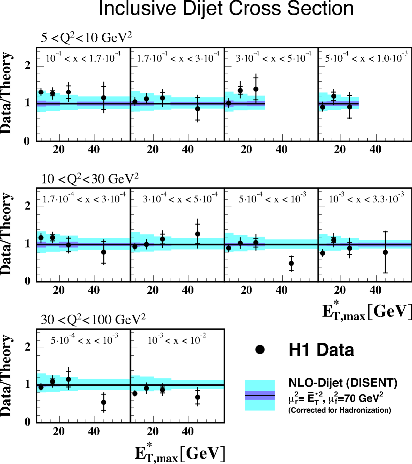
Figure 6: The ratio of the measured inclusive dijet cross section for $\Delta=2$ GeV to the theoretical prediction in bins of Bjorken-$x$, $Q^{2}$ and $E^{\ast}_{T,{\rm max}}$. The data are shown together with their statistical uncertainties (inner error bars) and their statistical and systematic uncertainties added in quadrature (outer error bars). They are compared with NLO dijet QCD predictions using the CTEQ6M parton distribution functions. The theoretical errors are given by the light error band representing the quadratic sum of the hadronization (dark error band) and renormalization scale uncertainties.

Measurements of the dijet cross section for $\Delta=2$ GeV as a function of $E^{\ast}_{T,{\rm max}}$ and $|\Delta\eta^{\ast}|$ in bins of Bjorken-$x$ and $Q^{2}$ are shown in Figures 4 and 5. Within the quoted uncertainties, good agreement between data and NLO calculations is observed, even at small values of $E^{\ast}_{T,{\rm max}}$ and $|\Delta\eta^{\ast}|$, i.e. in a kinematic region in which effects due to low-$x$ dynamics should be most prominent [17]. The level of agreement is more visible in Figures 6 and 7 which show the ratio of the data to the NLO predictions as a function of $E^{\ast}_{T,{\rm max}}$ and $|\Delta\eta^{\ast}|$ in bins of Bjorken-$x$ and $Q^{2}$.

The measured dijet cross sections are summarized in Tables 3 to 5. In addition, all dijet cross sections shown have been normalized to the total inclusive cross section for each bin. These dijet rates, $R_{2}=N_{\rm dijet}/N_{\rm DIS}$, are listed in Tables 6 to 8.

7.2 Azimuthal Jet Separation

Insight into low-$x$ dynamics can be gained from inclusive dijet data by studying the behavior of events with a small azimuthal separation, $\Delta\phi^{\ast}$, between the two hardest jets as measured in the hadronic center-of-mass system [18, 17, 16]. Partons entering the hard scattering process with negligible transverse momentum, $k_{t}$, as assumed in the DGLAP formalism, produce at leading order a back-to-back configuration of the two outgoing jets with $\Delta\phi^{\ast}\sim 180^{\circ}$. Azimuthal jet separations different from $180^{\circ}$ occur due to higher order QCD effects. However, in models which predict a significant proportion of partons entering the hard process with large $k_{t}$, the number of events with small $\Delta\phi^{\ast}$ increases. This is the case for the BFKL and CCFM evolution schemes. As an illustration, Figure 8 shows the uncorrected $\Delta\phi^{\ast}$ distribution for several intervals in $Q^{2}$. The expected steeply falling spectrum is observed with a tail extending to small values of $\Delta\phi^{\ast}$. This behavior is broadly reproduced by the Monte Carlo programs RAPGAP (direct) and ARIADNE, which are used to correct the data and estimate model uncertainties in the same manner as for the differential cross section measurements.

Large migrations connected with the limited hadronic energy resolution make an extraction of the dijet cross section at small $\Delta\phi^{\ast}$ rather difficult. Thus the ratio

$$S(\alpha)=\frac{\int^{\alpha}_{0}{N_{\rm dijet}(\Delta\phi^{*},x,Q^{2}){\rm d}\Delta\phi^{*}}}{\int^{180^{\circ}}_{0}{N_{\rm dijet}(\Delta\phi^{*},x,Q^{2}){\rm d}\Delta\phi^{*}}},$$

of the number of events $N_{\rm dijet}$ with an azimuthal jet separation of $\Delta\phi^{\ast}<\alpha$ relative to all dijet events is measured, as proposed in [16]. This variable is also directly sensitive to low-$x$ effects. For the analysis presented here $\alpha=120^{\circ}$ is chosen, which results in a purity of around 45% independently of $x$ and $Q^{2}$ and systematic uncertainties of similar size to those on the cross section measurements.

Figure 9 presents the $S$ distribution for $\alpha=120^{\circ}$ as a function of $x$ for different $Q^{2}$. The measured $S$ values are summarized in Table 9. For the chosen $\alpha$, the measured values of $S$ are of the order of 5% and increase with decreasing $x$. This rise of $S$ is most prominent in the lowest $Q^{2}$ bin, where the lowest values of $x$ are reached. The NLO dijet QCD calculations predict $S$ values of only $\sim$1% and show no rise towards low $x$. Low values of $S$ are expected for the NLO dijet predictions, since without any restrictions in acceptance, the two most energetic jets should always be separated by more than $\Delta\phi^{\ast}=120^{\circ}$. However, since selection criteria have to be applied to match the experimental conditions, non-vanishing $S$ values arise, due to event topologies for which some of the jets lie outside the analyzed phase space. In the same figure NLO 3-jet predictions are also shown. These give a good description of the data at large $Q^{2}$ and large $x$, but still fail to describe the increase towards low $x$, particularly in the lowest $Q^{2}$ range.

An informative comparison of the measured $S$ distribution with theory is also provided by models with different implementations of higher order QCD effects. Within the DGLAP approach such a model is provided for example by RAPGAP (direct). As shown in Figure 10, RAPGAP (direct) predicts a much larger ratio $S$ than the NLO dijet calculation. However, it still fails to describe the data in the low-$x$, low-$Q^{2}$ region. An improved description is achieved when resolved photon processes are included in RAPGAP (direct$+$resolved). Even with direct and resolved photon contributions included, RAPGAP fails to describe the data at very low $x$ and $Q^{2}$. Note that to obtain this overall level of agreement, it was necessary to choose a rather large scale, i.e. $\mu_{r}^{2}=Q^{2}+{\rm 4}\bar{{E}^{{}^{\ast}}_{T}}^{2}$, in order to get a large enough resolved photon contribution.

If the observed discrepancies are due to the influence of non-$k_{t}$-ordered parton emissions, models based on the color dipole model or CCFM evolution may provide a better description of the ratio $S$. In Figure 11 the data are therefore compared with the predictions of the ARIADNE and CASCADE Monte Carlo programs. For CASCADE, the two predictions presented are based on the JS2001 [37] and set 2 of the J2003 [46] unintegrated parton distributions, which differ in the way the small $k_{t}$ region is treated. For J2003 set 2, the full splitting function, including the non-singular term, is used, in contrast to JS2001, for which only the singular terms were considered. Whereas the prediction for $S$ using JS2001 lies significantly above the data, that based on set 2 of J2003 describes the data rather well. Note that both PDFs describe the H1 structure function data [24]. Hence, the measurement of the ratio $S$ improves the sensitivity to the details of the unintegrated gluon distribution. A good description of the $S$ distribution at low $x$ and low $Q^{2}$ is also provided by the color dipole model incorporated in ARIADNE. However, at higher $Q^{2}$ the ARIADNE prediction falls below the measured $S$ values.

8 Conclusion

Inclusive dijet production in deep inelastic $ep$ scattering is measured in the kinematic range $5<Q^{2}<100$ GeV², $10^{-4}<x<10^{-2}$ and $0.1<y<0.7$. Multi-differential cross section data are compared with NLO QCD predictions and no significant deviations are observed within the experimental and theoretical uncertainties. In the kinematic range studied, the next-to-leading order DGLAP approach thus provides an adequate theory for predicting $ep$ dijet cross sections as a function of Bjorken-$x$, $Q^{2}$, $E^{\ast}_{T,{\rm max}}$ and $|\Delta\eta^{\ast}|$.

NLO dijet QCD calculations predict values that are much too low for the ratio, $S$, of events with a small azimuthal separation of the two highest transverse momentum jets with respect to the total number of inclusive dijet events. The additional hard emission, provided by the NLO 3-jet calculations, considerably improves the description of the data, but is insufficient at low $x$ and low $Q^{2}$. A similar description of the data is provided by RAPGAP, a DGLAP-based QCD model, which matches LO matrix elements for direct and resolved processes to $k_{t}$-ordered parton cascades. A good description of the measured ratio $S$ at low $x$ and $Q^{2}$ is given by the ARIADNE program, which generates non-$k_{t}$-ordered parton cascades using the color dipole model. Predictions based on the CCFM evolution equations and $k_{t}$ factorized unintegrated gluon densities are provided by the CASCADE Monte Carlo program. Large differences are found between the predictions for two different choices of the unintegrated gluon density, both of which describe the H1 structure function data and one of which gives a good description of $S$. This measurement thus provides a significant constraint on the unintegrated gluon density.

Figure 1: Leading order diagrams for dijet production in $ep$ scattering. (a) photon-gluon fusion and (b) QCD-Compton process. (c) parton cascade diagram: $k_{t}$ denotes the transverse momenta of the exchanged gluons, $x_{g}$ the fractional longitudinal momentum of the gluon taking part in the hard process and $x$ is the Bjorken scaling variable.

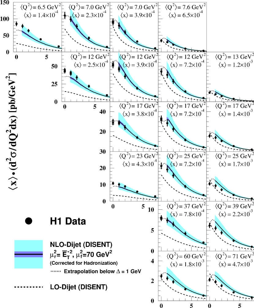
Figure 2: Inclusive dijet cross section as given in Table 3, multiplied by $\langle x\rangle$ and averaged over $x$ and $Q^{2}$, as a function of $\Delta$, defined by the requirement $E^{\ast}_{T,1}\equiv E^{\ast}_{T,{\rm max}}>({\rm 5}+\Delta)$ GeV. Here $\langle x\rangle$ and $\langle Q^{2}\rangle$ are the mean values of Bjorken-$x$ and $Q^{2}$ for fully inclusive events in a given bin. The data are shown together with their statistical uncertainties (inner error bars) and their statistical and systematic uncertainties added in quadrature (outer error bars). They are compared with NLO (LO) dijet QCD predictions using the CTEQ6M (CTEQ6L) parton distribution functions. The NLO predictions are corrected for hadronization effects. The outer light error band includes the quadratic sum of hadronization (dark error band) and renormalization scale uncertainties on the NLO predictions.

Figure 3: Inclusive dijet cross section averaged over $Q^{2}$ and Bjorken-$x$ for $\Delta=2$ GeV (see text). The data are plotted at the center of each bin and are shown with their statistical uncertainties (inner error bars) and their statistical and systematic uncertainties added in quadrature (outer error bars). They are compared with NLO (LO) dijet QCD predictions using the CTEQ6M (CTEQ6L) parton distribution functions. The NLO predictions are corrected for hadronization effects. The outer light error band includes the quadratic sum of hadronization (dark error band) and renormalization scale uncertainties on the NLO predictions.

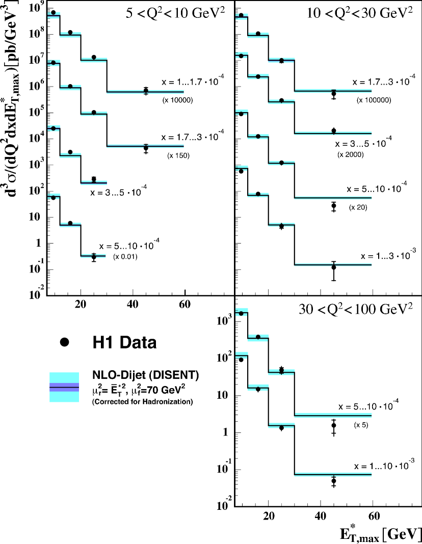
Figure 4: Inclusive dijet cross section for $\Delta=2$ GeV averaged over Bjorken-$x$, $Q^{2}$ and $E^{\ast}_{T,{\rm max}}$ as given in Table 4, compared with NLO dijet QCD predictions using the CTEQ6M parton distribution functions. The data are plotted at the center of each bin and are shown together with their statistical uncertainties (inner error bars) and their statistical and systematic uncertainties added in quadrature (outer error bars). The NLO predictions are corrected for hadronization effects. The outer light error band includes the quadratic sum of hadronization (dark error band) and renormalization scale uncertainties on the NLO predictions.

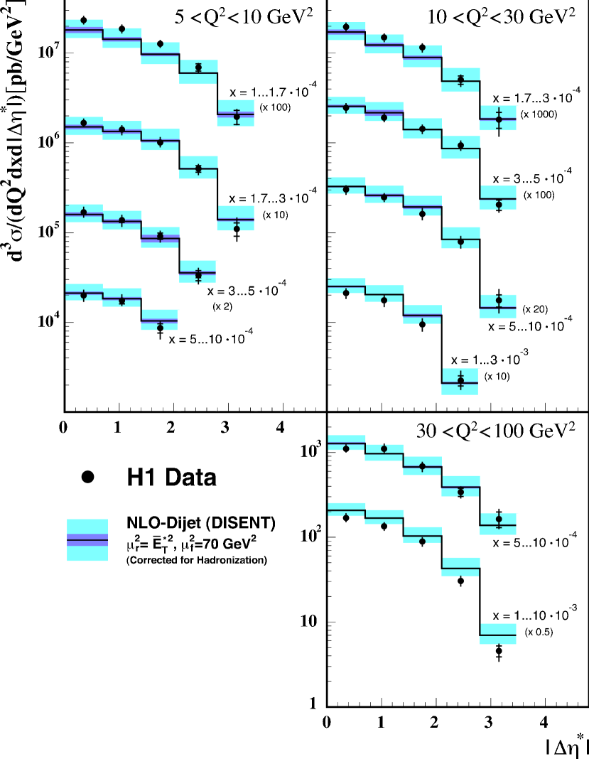
Figure 5: Inclusive dijet cross section for $\Delta=2$ GeV averaged over Bjorken-$x$, $Q^{2}$ and the pseudorapidity distance $|\Delta\eta^{\ast}|$ between the dijets as given in Table 5, compared with NLO dijet QCD predictions using the CTEQ6M parton distribution functions. The data are plotted at the center of each bin and are shown together with their statistical uncertainties (inner error bars) and their statistical and systematic uncertainties added in quadrature (outer error bars). The NLO predictions are corrected for hadronization effects. The outer light error band includes the quadratic sum of hadronization (dark error band) and renormalization scale uncertainties on the NLO predictions.

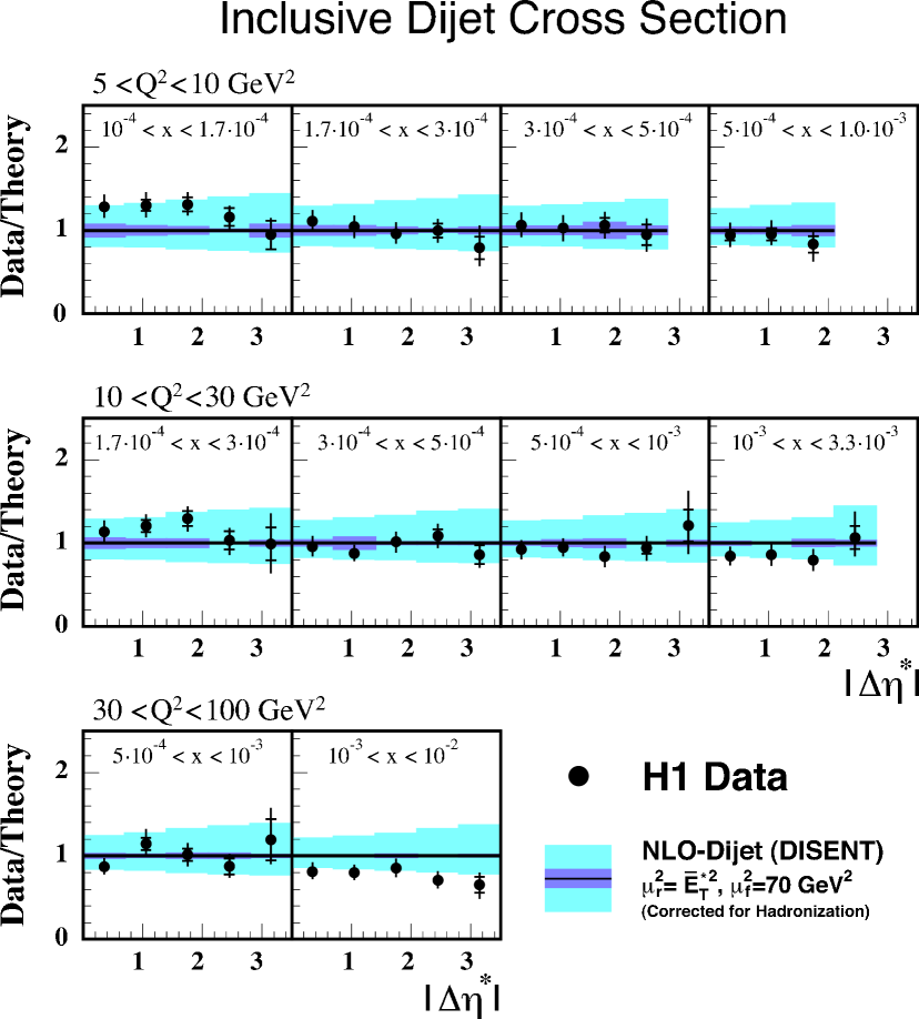
Figure 7: The ratio of the measured inclusive dijet cross section for $\Delta=2$ GeV to the theoretical prediction in bins of Bjorken-$x$, $Q^{2}$ and $|\Delta\eta^{\ast}|$. The data are shown together with their statistical uncertainties (inner error bars) and their statistical and systematic uncertainties added in quadrature (outer error bars). They are compared with NLO dijet QCD predictions using the CTEQ6M parton distribution functions. The theoretical errors are given by the light error band representing the quadratic sum of the hadronization (dark error band) and renormalization scale uncertainties.

Figure 8: Normalized measured event distributions as a function of the azimuthal separation, $\Delta\phi^{*}$, between the two highest transverse momentum jets. The data are shown for different regions in $Q^{2}$ and are compared with two Monte Carlo models, ARIADNE and RAPGAP.

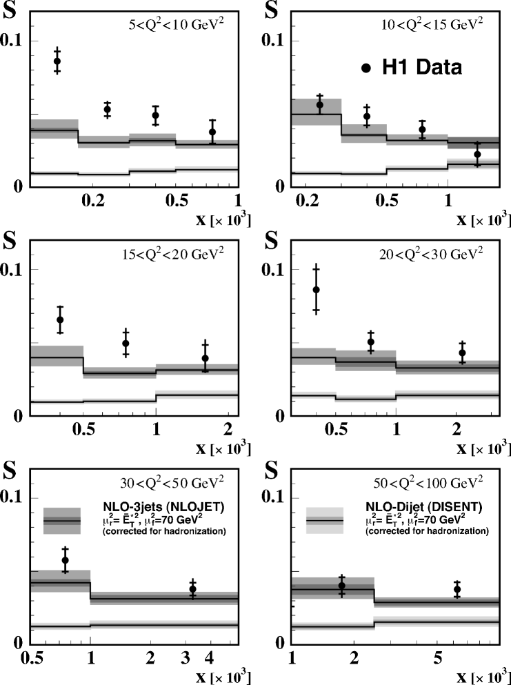
Figure 9: Ratio $S$ of the number of events with a small azimuthal jet separation ($\Delta\phi^{\ast}<120^{\circ}$) between the two highest transverse momentum jets with respect to the total number of inclusive dijet events, as a function of Bjorken-$x$ and $Q^{2}$. The data are plotted at the center of each bin and are shown together with their statistical uncertainties (inner error bars) and their statistical and systematic uncertainties added in quadrature (outer error bars). The data are compared with NLO QCD predictions for dijet and 3-jet production using the CTEQ6M parton distribution functions. The theoretical errors are given by the light error band representing the quadratic sum of the hadronization (dark error band) and renormalization scale uncertainties.

Figure 10: Ratio $S$ of the number of events with a small azimuthal jet separation ($\Delta\phi^{\ast}<120^{\circ}$) between the two highest transverse momentum jets with respect to the total number of inclusive dijet events, as a function of Bjorken-$x$ and $Q^{2}$. The data are plotted at the center of each bin and are shown together with their statistical uncertainties (inner error bars) and their statistical and systematic uncertainties added in quadrature (outer error bars). The data are compared with predictions from the RAPGAP generator, both with direct photons alone (full line) and with direct and resolved contributions (dashed line).

Figure 11: Ratio $S$ of the number of events with a small azimuthal jet separation ($\Delta\phi^{\ast}<120^{\circ}$) between the two highest transverse momentum jets with respect to the total number of inclusive dijet events, as function of Bjorken-$x$ and $Q^{2}$ . The data are plotted at the center of each bin and are shown together with their statistical uncertainties (inner error bars) and their statistical and systematic uncertainties added in quadrature (outer error bars). They are compared with predictions from a model based on CCFM evolution (CASCADE) and using two different $k_{t}$-unintegrated gluon distribution functions, JS2001 (full line) and set 2 of J2003 (dashed line). In addition, the data are compared with predictions based on the color dipole model (ARIADNE), which produces $k_{t}$-unordered parton showers.

$Q^{2}$			$x/10^{-4}$			$\Delta$	$\frac{d^{2}\sigma}{dQ^{2}dx}$	$\delta_{stat}$	$\delta_{syst.}$
$\rm\ [GeV^{2}]$						$\rm\ [GeV]$	$\rm\ [pb/GeV^{2}]$	$[\%]$	$[\%]$
$\rule[-0.28453pt]{0.0pt}{8.53581pt}5.0$	–	$10.0$	$1.0$	–	$1.7$	$0$	$6.1\cdot 10^{5}$	3	8
						$1$	$5.6\cdot 10^{5}$	3	7
						$2$	$4.6\cdot 10^{5}$	3	7
						$4$	$2.7\cdot 10^{5}$	4	8
						$7$	$1.2\cdot 10^{5}$	6	9
			$\rule[-0.28453pt]{0.0pt}{8.53581pt}1.7$	–	$3.0$	$0$	$4.8\cdot 10^{5}$	3	9
						$1$	$4.3\cdot 10^{5}$	3	10
						$2$	$3.4\cdot 10^{5}$	3	9
						$4$	$1.8\cdot 10^{5}$	4	9
						$7$	$6.6\cdot 10^{4}$	5	11
			$\rule[-0.28453pt]{0.0pt}{8.53581pt}3.0$	–	$5.0$	$0$	$2.3\cdot 10^{5}$	4	12
						$1$	$2.0\cdot 10^{5}$	4	12
						$2$	$1.5\cdot 10^{5}$	4	11
						$4$	$8.0\cdot 10^{4}$	5	11
						$7$	$2.9\cdot 10^{4}$	8	13
			$\rule[-0.28453pt]{0.0pt}{8.53581pt}5.0$	–	$10.0$	$0$	$5.2\cdot 10^{4}$	5	14
						$1$	$4.6\cdot 10^{4}$	5	13
						$2$	$3.4\cdot 10^{4}$	5	13
						$4$	$1.6\cdot 10^{4}$	7	12
						$7$	$5.4\cdot 10^{3}$	10	15
$\rule[-0.28453pt]{0.0pt}{8.53581pt}10.0$	–	$15.0$	$1.7$	–	$3.0$	$0$	$1.7\cdot 10^{5}$	4	8
						$1$	$1.6\cdot 10^{5}$	4	8
						$2$	$1.4\cdot 10^{5}$	4	9
						$4$	$8.7\cdot 10^{4}$	5	9
						$7$	$3.7\cdot 10^{4}$	7	8
			$\rule[-0.28453pt]{0.0pt}{8.53581pt}3.0$	–	$5.0$	$0$	$1.3\cdot 10^{5}$	3	10
						$1$	$1.2\cdot 10^{5}$	3	9
						$2$	$9.1\cdot 10^{4}$	4	9
						$4$	$4.8\cdot 10^{4}$	5	10
						$7$	$2.0\cdot 10^{4}$	7	11
			$\rule[-0.28453pt]{0.0pt}{8.53581pt}5.0$	–	$10.0$	$0$	$5.9\cdot 10^{4}$	3	13
						$1$	$5.2\cdot 10^{4}$	3	12
						$2$	$4.0\cdot 10^{4}$	4	12
						$4$	$2.0\cdot 10^{4}$	5	12
						$7$	$7.3\cdot 10^{3}$	7	13
			$\rule[-0.28453pt]{0.0pt}{8.53581pt}10.0$	–	$18.0$	$0$	$1.1\cdot 10^{4}$	6	12
						$1$	$8.8\cdot 10^{3}$	7	13
						$2$	$6.4\cdot 10^{3}$	7	15
						$4$	$3.3\cdot 10^{3}$	9	15
						$7$	$9.3\cdot 10^{2}$	17	22

Table 3: Inclusive dijet cross section averaged over the regions indicated in $x$ and $Q^{2}$, for different values of $\Delta$ as shown in Figures 2 and 3. The measurement is restricted to values of the inelasticity variable $y$ between $0.1<y<0.7$ and to values of the polar angle of the scattered electron between $156^{\circ}<\theta<175^{\circ}$.

$Q^{2}$			$x/10^{-4}$			$\Delta$	$\frac{d^{2}\sigma}{dQ^{2}dx}$	$\delta_{stat}$	$\delta_{syst.}$
$\rm\ [GeV^{2}]$						$\rm\ [GeV]$	$\rm\ [pb/GeV^{2}]$	$[\%]$	$[\%]$
$\rule[-0.28453pt]{0.0pt}{8.53581pt}15.0$	–	$20.0$	$3.0$	–	$5.0$	$0$	$7.8\cdot 10^{4}$	6	9
						$1$	$7.6\cdot 10^{4}$	4	9
						$2$	$6.4\cdot 10^{4}$	4	9
						$4$	$3.7\cdot 10^{4}$	5	9
						$7$	$1.5\cdot 10^{4}$	7	10
			$\rule[-0.28453pt]{0.0pt}{8.53581pt}5.0$	–	$10.0$	$0$	$4.5\cdot 10^{4}$	4	11
						$1$	$4.0\cdot 10^{4}$	4	12
						$2$	$3.1\cdot 10^{4}$	4	11
						$4$	$1.6\cdot 10^{4}$	5	11
						$7$	$5.8\cdot 10^{3}$	8	12
			$\rule[-0.28453pt]{0.0pt}{8.53581pt}10.0$	–	$22.0$	$0$	$1.1\cdot 10^{4}$	5	12
						$1$	$9.9\cdot 10^{3}$	5	13
						$2$	$7.6\cdot 10^{3}$	5	12
						$4$	$3.8\cdot 10^{3}$	7	13
						$7$	$1.3\cdot 10^{3}$	11	15
$\rule[-0.28453pt]{0.0pt}{8.53581pt}20.0$	–	$30.0$	$3.0$	–	$5.0$	$0$	$2.5\cdot 10^{4}$	5	8
						$1$	$2.4\cdot 10^{4}$	5	8
						$2$	$2.1\cdot 10^{4}$	5	9
						$4$	$1.4\cdot 10^{4}$	6	8
						$7$	$6.7\cdot 10^{3}$	9	9
			$\rule[-0.28453pt]{0.0pt}{8.53581pt}5.0$	–	$10.0$	$0$	$2.9\cdot 10^{4}$	3	9
						$1$	$2.7\cdot 10^{4}$	3	9
						$2$	$2.1\cdot 10^{4}$	3	10
						$4$	$1.2\cdot 10^{4}$	4	10
						$7$	$5.1\cdot 10^{3}$	6	10
			$\rule[-0.28453pt]{0.0pt}{8.53581pt}10.0$	–	$33.0$	$0$	$6.2\cdot 10^{3}$	3	11
						$1$	$5.5\cdot 10^{3}$	3	11
						$2$	$4.1\cdot 10^{3}$	3	11
						$4$	$2.2\cdot 10^{3}$	4	12
						$7$	$9.3\cdot 10^{2}$	7	13
$\rule[-0.28453pt]{0.0pt}{8.53581pt}30.0$	–	$50.0$	$5.0$	–	$10.0$	$0$	$1.0\cdot 10^{4}$	3	8
						$1$	$9.5\cdot 10^{3}$	3	8
						$2$	$8.2\cdot 10^{3}$	4	10
						$4$	$5.4\cdot 10^{3}$	4	9
						$7$	$2.6\cdot 10^{3}$	6	10
			$\rule[-0.28453pt]{0.0pt}{8.53581pt}10.0$	–	$55.0$	$0$	$2.8\cdot 10^{3}$	2	10
						$1$	$2.5\cdot 10^{3}$	2	10
						$2$	$2.0\cdot 10^{3}$	3	11
						$4$	$1.1\cdot 10^{3}$	3	12
						$7$	$4.7\cdot 10^{2}$	5	13
$\rule[-0.28453pt]{0.0pt}{8.53581pt}50.0$	–	$100.0$	$10.0$	–	$25.0$	$0$	$1.4\cdot 10^{3}$	3	9
						$1$	$1.3\cdot 10^{3}$	3	9
						$2$	$1.1\cdot 10^{3}$	3	9
						$4$	$6.5\cdot 10^{2}$	4	10
						$7$	$2.8\cdot 10^{2}$	6	13
			$\rule[-0.28453pt]{0.0pt}{8.53581pt}25.0$	–	$100.0$	$0$	$4.5\cdot 10^{2}$	3	9
						$1$	$4.0\cdot 10^{2}$	3	10
						$2$	$3.2\cdot 10^{2}$	3	11
						$4$	$1.8\cdot 10^{2}$	4	11
						$7$	$7.1\cdot 10^{1}$	6	17

Table 3 continued.

$Q^{2}$			$x/10^{-4}$			$E^{\ast}_{T,max}$			$\frac{d^{3}\sigma}{dQ^{2}dxdE^{\ast}_{T,max}}$	$\delta_{stat}$	$\delta_{syst.}$
$\rm\ [GeV^{2}]$						$\rm\ [GeV]$			$\rm\ [pb/GeV^{3}]$	$[\%]$	$[\%]$
$\rule[-0.28453pt]{0.0pt}{14.22636pt}5.0$	–	$10.0$	$1.0$	–	$1.7$	$7.0$	–	$12.0$	$6.8\cdot 10^{4\phantom{-}}$	4	9
						$12.0$	–	$20.0$	$1.2\cdot 10^{4\phantom{-}}$	6	12
						$20.0$	–	$30.0$	$1.3\cdot 10^{3\phantom{-}}$	13	16
						$30.0$	–	$60.0$	$7.2\cdot 10^{1\phantom{-}}$	27	27
			$\rule[-0.28453pt]{0.0pt}{14.22636pt}1.7$	–	$3.0$	$7.0$	–	$12.0$	$5.5\cdot 10^{4\phantom{-}}$	3	11
						$12.0$	–	$20.0$	$6.8\cdot 10^{3\phantom{-}}$	5	14
						$20.0$	–	$30.0$	$6.9\cdot 10^{2\phantom{-}}$	13	17
						$30.0$	–	$60.0$	$3.0\cdot 10^{1\phantom{-}}$	35	25
			$\rule[-0.28453pt]{0.0pt}{14.22636pt}3.0$	–	$5.0$	$7.0$	–	$12.0$	$2.5\cdot 10^{4\phantom{-}}$	4	12
						$12.0$	–	$20.0$	$3.1\cdot 10^{3\phantom{-}}$	8	17
						$20.0$	–	$30.0$	$2.9\cdot 10^{2\phantom{-}}$	21	21
			$\rule[-0.28453pt]{0.0pt}{14.22636pt}5.0$	–	$10.0$	$7.0$	–	$12.0$	$5.6\cdot 10^{3\phantom{-}}$	5	15
						$12.0$	–	$20.0$	$6.0\cdot 10^{2\phantom{-}}$	10	17
						$20.0$	–	$30.0$	$3.0\cdot 10^{1\phantom{-}}$	33	30
$\rule[-0.28453pt]{0.0pt}{14.22636pt}10.0$	–	$30.0$	$1.7$	–	$3.0$	$7.0$	–	$12.0$	$5.5\cdot 10^{3\phantom{-}}$	6	11
						$12.0$	–	$20.0$	$1.1\cdot 10^{3\phantom{-}}$	7	12
						$20.0$	–	$30.0$	$1.0\cdot 10^{2\phantom{-}}$	18	14
						$30.0$	–	$60.0$	$5.4\cdot 10^{0\phantom{-}}$	36	22
			$\rule[-0.28453pt]{0.0pt}{14.22636pt}3.0$	–	$5.0$	$7.0$	–	$12.0$	$7.4\cdot 10^{3\phantom{-}}$	3	11
						$12.0$	–	$20.0$	$1.2\cdot 10^{3\phantom{-}}$	5	13
						$20.0$	–	$30.0$	$1.5\cdot 10^{2\phantom{-}}$	11	18
						$30.0$	–	$60.0$	$1.0\cdot 10^{1\phantom{-}}$	20	25
			$\rule[-0.28453pt]{0.0pt}{14.22636pt}5.0$	–	$1.0$	$7.0$	–	$12.0$	$4.6\cdot 10^{3\phantom{-}}$	2	12
						$12.0$	–	$20.0$	$6.2\cdot 10^{2\phantom{-}}$	4	15
						$20.0$	–	$30.0$	$6.1\cdot 10^{1\phantom{-}}$	11	18
						$30.0$	–	$60.0$	$1.4\cdot 10^{0\phantom{-}}$	36	24
			$\rule[-0.28453pt]{0.0pt}{14.22636pt}1.0$	–	$33.0$	$7.0$	–	$12.0$	$5.7\cdot 10^{2\phantom{-}}$	3	14
						$12.0$	–	$20.0$	$7.8\cdot 10^{1\phantom{-}}$	6	16
						$20.0$	–	$30.0$	$4.6\cdot 10^{0\phantom{-}}$	18	26
						$30.0$	–	$60.0$	$0.1\cdot 10^{0\phantom{-}}$	69	23
$\rule[-0.28453pt]{0.0pt}{14.22636pt}30.0$	–	$100.0$	$5.0$	–	$10.0$	$7.0$	–	$12.0$	$3.3\cdot 10^{2\phantom{-}}$	4	11
						$12.0$	–	$20.0$	$7.8\cdot 10^{1\phantom{-}}$	6	14
						$20.0$	–	$30.0$	$9.7\cdot 10^{0\phantom{-}}$	17	24
						$30.0$	–	$60.0$	$0.3\cdot 10^{0\phantom{-}}$	39	32
			$\rule[-0.28453pt]{0.0pt}{14.22636pt}10.0$	–	$100.0$	$7.0$	–	$12.0$	$9.3\cdot 10^{1\phantom{-}}$	2	11
						$12.0$	–	$20.0$	$1.5\cdot 10^{1\phantom{-}}$	3	17
						$20.0$	–	$30.0$	$1.3\cdot 10^{0\phantom{-}}$	9	18
						$30.0$	–	$60.0$	$5.0\cdot 10^{-2}$	26	30

Table 4: Inclusive dijet cross section averaged over the regions indicated in $x$, $Q^{2}$ and $E^{\ast}_{T,max}$ for $\Delta=2$ GeV as shown in Figure 4. The measurement is restricted to values of the inelasticity variable $y$ between $0.1<y<0.7$ and to values of the polar angle of the scattered electron between $156^{\circ}<\theta<175^{\circ}$.

$Q^{2}$			$x/10^{-4}$			$|\Delta\eta^{\ast}|$			$\frac{d^{3}\sigma}{dQ^{2}dxd|\Delta\eta^{\ast}|}$	$\delta_{stat}$	$\delta_{syst.}$
$\rm\ [GeV^{2}]$									$\rm\ [pb/GeV^{2}]$	$[\%]$	$[\%]$
$\rule[-0.28453pt]{0.0pt}{9.95845pt}5.0$	–	$10.0$	$1.0$	–	$1.7$	$0.0$	–	$0.7$	$2.3\cdot 10^{5}$	4	10
						$0.7$	–	$1.4$	$1.9\cdot 10^{5}$	5	11
						$1.4$	–	$2.1$	$1.3\cdot 10^{5}$	6	9
						$2.1$	–	$2.8$	$7.0\cdot 10^{4}$	9	9
						$2.8$	–	$3.5$	$2.0\cdot 10^{4}$	18	13
			$\rule[-0.28453pt]{0.0pt}{9.95845pt}1.7$	–	$3.0$	$0.0$	–	$0.7$	$1.7\cdot 10^{5}$	4	12
						$0.7$	–	$1.4$	$1.4\cdot 10^{5}$	4	12
						$1.4$	–	$2.1$	$1.0\cdot 10^{5}$	6	14
						$2.1$	–	$2.8$	$5.1\cdot 10^{4}$	8	12
						$2.8$	–	$3.5$	$1.1\cdot 10^{4}$	17	30
			$\rule[-0.28453pt]{0.0pt}{9.95845pt}3.0$	–	$5.0$	$0.0$	–	$0.7$	$8.5\cdot 10^{4}$	5	14
						$0.7$	–	$1.4$	$6.9\cdot 10^{4}$	6	15
						$1.4$	–	$2.1$	$4.6\cdot 10^{4}$	8	13
						$2.1$	–	$2.8$	$1.7\cdot 10^{4}$	13	17
			$\rule[-0.28453pt]{0.0pt}{9.95845pt}5.0$	–	$10.0$	$0.0$	–	$0.7$	$2.0\cdot 10^{4}$	7	14
						$0.7$	–	$1.4$	$1.7\cdot 10^{4}$	8	16
						$1.4$	–	$2.1$	$8.6\cdot 10^{3}$	12	22
$\rule[-0.28453pt]{0.0pt}{9.95845pt}10.0$	–	$30.0$	$1.7$	–	$3.0$	$0.0$	–	$0.7$	$2.0\cdot 10^{4}$	5	13
						$0.7$	–	$1.4$	$1.5\cdot 10^{4}$	6	10
						$1.4$	–	$2.1$	$1.2\cdot 10^{4}$	7	10
						$2.1$	–	$2.8$	$5.0\cdot 10^{3}$	11	13
						$2.8$	–	$3.5$	$1.8\cdot 10^{3}$	20	31
			$\rule[-0.28453pt]{0.0pt}{9.95845pt}3.0$	–	$5.0$	$0.0$	–	$0.7$	$2.5\cdot 10^{4}$	4	12
						$0.7$	–	$1.4$	$1.9\cdot 10^{4}$	4	11
						$1.4$	–	$2.1$	$1.4\cdot 10^{4}$	5	11
						$2.1$	–	$2.8$	$9.4\cdot 10^{3}$	7	11
						$2.8$	–	$3.5$	$2.0\cdot 10^{3}$	13	13
			$\rule[-0.28453pt]{0.0pt}{9.95845pt}5.0$	–	$1.0$	$0.0$	–	$0.7$	$1.5\cdot 10^{4}$	3	12
						$0.7$	–	$1.4$	$1.2\cdot 10^{4}$	3	12
						$1.4$	–	$2.1$	$8.1\cdot 10^{3}$	5	15
						$2.1$	–	$2.8$	$4.0\cdot 10^{3}$	7	14
						$2.8$	–	$3.5$	$8.8\cdot 10^{2}$	16	30
			$\rule[-0.28453pt]{0.0pt}{9.95845pt}1.0$	–	$33.0$	$0.0$	–	$0.7$	$2.1\cdot 10^{3}$	4	13
						$0.7$	–	$1.4$	$1.8\cdot 10^{3}$	4	15
						$1.4$	–	$2.1$	$9.5\cdot 10^{2}$	7	16
						$2.1$	–	$2.8$	$2.2\cdot 10^{2}$	13	26
$\rule[-0.28453pt]{0.0pt}{9.95845pt}30.0$	–	$100.0$	$5.0$	–	$10.0$	$0.0$	–	$0.7$	$1.1\cdot 10^{3}$	6	11
						$0.7$	–	$1.4$	$1.1\cdot 10^{3}$	6	14
						$1.4$	–	$2.1$	$6.8\cdot 10^{2}$	7	12
						$2.1$	–	$2.8$	$3.4\cdot 10^{2}$	11	13
						$2.8$	–	$3.5$	$1.6\cdot 10^{2}$	21	24
			$\rule[-0.28453pt]{0.0pt}{9.95845pt}10.0$	–	$100.0$	$0.0$	–	$0.7$	$3.4\cdot 10^{2}$	3	14
						$0.7$	–	$1.4$	$2.7\cdot 10^{2}$	3	11
						$1.4$	–	$2.1$	$1.8\cdot 10^{2}$	4	13
						$2.1$	–	$2.8$	$6.1\cdot 10^{1}$	6	14
						$2.8$	–	$3.5$	$9.1\cdot 10^{0}$	15	21

Table 5: Inclusive dijet cross section averaged over the regions indicated in $x$, $Q^{2}$ and $|\Delta\eta^{\ast}|$ for $\Delta=2$ GeV as shown in Figure 5. The measurement is restricted to values of the inelasticity variable $y$ between $0.1<y<0.7$ and to values of the polar angle of the scattered electron between $156^{\circ}<\theta<175^{\circ}$.

$Q^{2}$			$x/10^{-4}$			$\Delta$	$R_{2}=\frac{N_{dijet}}{N_{DIS}}$	$\delta_{stat}$	$\delta_{syst.}$
$\rm\ [GeV^{2}]$						$\rm\ [GeV]$		$[\%]$	$[\%]$
$\rule[-0.28453pt]{0.0pt}{8.53581pt}5.0$	–	$10.0$	$1.0$	–	$1.7$	$0$	0.031	4	9
						$1$	0.028	4	9
						$2$	0.023	3	9
						$4$	0.014	4	9
						$7$	0.006	6	10
			$\rule[-0.28453pt]{0.0pt}{8.53581pt}1.7$	–	$3.0$	$0$	0.027	3	9
						$1$	0.024	3	9
						$2$	0.019	3	9
						$4$	0.010	4	10
						$7$	0.004	5	12
			$\rule[-0.28453pt]{0.0pt}{8.53581pt}3.0$	–	$5.0$	$0$	0.021	4	12
						$1$	0.019	4	12
						$2$	0.014	4	11
						$4$	0.007	5	11
						$7$	0.003	8	13
			$\rule[-0.28453pt]{0.0pt}{8.53581pt}5.0$	–	$10.0$	$0$	0.015	5	15
						$1$	0.013	5	14
						$2$	0.010	5	14
						$4$	0.004	7	14
						$7$	0.002	10	18
$\rule[-0.28453pt]{0.0pt}{8.53581pt}10.0$	–	$15.0$	$1.7$	–	$3.0$	$0$	0.040	4	8
						$1$	0.037	4	8
						$2$	0.031	4	9
						$4$	0.020	5	10
						$7$	0.009	7	9
			$\rule[-0.28453pt]{0.0pt}{8.53581pt}3.0$	–	$5.0$	$0$	0.035	3	10
						$1$	0.031	3	9
						$2$	0.024	4	9
						$4$	0.013	5	10
						$7$	0.005	7	11
			$\rule[-0.28453pt]{0.0pt}{8.53581pt}5.0$	–	$10.0$	$0$	0.027	3	13
						$1$	0.024	4	12
						$2$	0.018	4	13
						$4$	0.009	5	13
						$7$	0.003	7	14
			$\rule[-0.28453pt]{0.0pt}{8.53581pt}10.0$	–	$18.0$	$0$	0.019	6	15
						$1$	0.016	7	14
						$2$	0.011	7	18
						$4$	0.006	9	20
						$7$	0.002	17	24

Table 6: Dijet rate $R_{2}$ averaged over the regions indicated in $Q^{2}$ and $x$ for different values of $\Delta$. The measurement is restricted to values of the inelasticity variable $y$ between $0.1<y<0.7$ and to values of the polar angle of the scattered electron between $156^{\circ}<\theta<175^{\circ}$.

$Q^{2}$			$x/10^{-4}$			$\Delta$	$R_{2}=\frac{N_{dijet}}{N_{DIS}}$	$\delta_{stat}$	$\delta_{syst.}$
$\rm\ [GeV^{2}]$						$\rm\ [GeV]$		$[\%]$	$[\%]$
$\rule[-0.28453pt]{0.0pt}{8.53581pt}15.0$	–	$20.0$	$3.0$	–	$5.0$	$0$	0.043	6	9
						$1$	0.042	4	8
						$2$	0.035	4	9
						$4$	0.020	5	9
						$7$	0.008	7	10
			$\rule[-0.28453pt]{0.0pt}{8.53581pt}5.0$	–	$10.0$	$0$	0.041	4	10
						$1$	0.036	4	12
						$2$	0.028	4	11
						$4$	0.015	5	10
						$7$	0.005	8	12
			$\rule[-0.28453pt]{0.0pt}{8.53581pt}10.0$	–	$22.0$	$0$	0.027	5	13
						$1$	0.024	5	13
						$2$	0.019	5	12
						$4$	0.009	7	14
						$7$	0.003	11	17
$\rule[-0.28453pt]{0.0pt}{8.53581pt}20.0$	–	$30.0$	$3.0$	–	$5.0$	$0$	0.056	5	8
						$1$	0.052	5	8
						$2$	0.046	6	8
						$4$	0.030	7	9
						$7$	0.015	9	10
			$\rule[-0.28453pt]{0.0pt}{8.53581pt}5.0$	–	$10.0$	$0$	0.054	3	9
						$1$	0.049	3	9
						$2$	0.040	3	9
						$4$	0.023	4	10
						$7$	0.010	6	10
			$\rule[-0.28453pt]{0.0pt}{8.53581pt}10.0$	–	$33.0$	$0$	0.038	3	11
						$1$	0.033	3	11
						$2$	0.025	4	12
						$4$	0.014	4	13
						$7$	0.006	7	15
$\rule[-0.28453pt]{0.0pt}{8.53581pt}30.0$	–	$50.0$	$5.0$	–	$10.0$	$0$	0.068	3	8
						$1$	0.064	3	8
						$2$	0.056	4	9
						$4$	0.036	4	9
						$7$	0.018	6	10
			$\rule[-0.28453pt]{0.0pt}{8.53581pt}10.0$	–	$55.0$	$0$	0.056	2	10
						$1$	0.051	2	10
						$2$	0.041	3	11
						$4$	0.023	3	12
						$7$	0.009	5	13
$\rule[-0.28453pt]{0.0pt}{8.53581pt}50.0$	–	$100.0$	$10.0$	–	$25.0$	$0$	0.087	3	9
						$1$	0.080	3	8
						$2$	0.067	3	9
						$4$	0.041	4	10
						$7$	0.018	6	13
			$\rule[-0.28453pt]{0.0pt}{8.53581pt}25.0$	–	$100.0$	$0$	0.072	3	9
						$1$	0.065	3	10
						$2$	0.052	3	11
						$4$	0.029	4	12
						$7$	0.011	6	18

Table 6 continued.

$Q^{2}$			$x/10^{-4}$			$E^{\ast}_{T,max}$			$\frac{dR_{2}}{dE^{\ast}_{T,max}}$	$\delta_{stat}$	$\delta_{syst.}$
$\rm\ [GeV^{2}]$						$\rm\ [GeV]$			$\rm\ [GeV^{-1}]$	$[\%]$	$[\%]$
$\rule[-0.28453pt]{0.0pt}{14.22636pt}5.0$	–	$10.0$	$1.0$	–	$1.7$	$7.0$	–	$12.0$	$3.5\cdot 10^{-3}$	3	10
						$12.0$	–	$20.0$	$4.9\cdot 10^{-4}$	6	14
						$20.0$	–	$30.0$	$6.8\cdot 10^{-5}$	13	18
						$30.0$	–	$60.0$	$3.6\cdot 10^{-6}$	27	27
			$\rule[-0.28453pt]{0.0pt}{14.22636pt}1.7$	–	$3.0$	$7.0$	–	$12.0$	$3.1\cdot 10^{-3}$	3	11
						$12.0$	–	$20.0$	$3.1\cdot 10^{-4}$	5	14
						$20.0$	–	$30.0$	$4.0\cdot 10^{-5}$	13	18
						$30.0$	–	$60.0$	$1.7\cdot 10^{-6}$	35	25
			$\rule[-0.28453pt]{0.0pt}{14.22636pt}3.0$	–	$5.0$	$7.0$	–	$12.0$	$2.3\cdot 10^{-3}$	4	13
						$12.0$	–	$20.0$	$2.3\cdot 10^{-4}$	8	17
						$20.0$	–	$30.0$	$2.6\cdot 10^{-5}$	21	22
			$\rule[-0.28453pt]{0.0pt}{14.22636pt}5.0$	–	$10.0$	$7.0$	–	$12.0$	$1.6\cdot 10^{-3}$	5	16
						$12.0$	–	$20.0$	$1.4\cdot 10^{-4}$	10	20
						$20.0$	–	$30.0$	$7.8\cdot 10^{-6}$	34	36
$\rule[-0.28453pt]{0.0pt}{14.22636pt}10.0$	–	$30.0$	$1.7$	–	$3.0$	$7.0$	–	$12.0$	$4.6\cdot 10^{-3}$	5	11
						$12.0$	–	$20.0$	$7.2\cdot 10^{-4}$	7	13
						$20.0$	–	$30.0$	$8.6\cdot 10^{-5}$	18	15
						$30.0$	–	$60.0$	$4.5\cdot 10^{-6}$	36	23
			$\rule[-0.28453pt]{0.0pt}{14.22636pt}3.0$	–	$5.0$	$7.0$	–	$12.0$	$4.6\cdot 10^{-3}$	3	11
						$12.0$	–	$20.0$	$5.9\cdot 10^{-4}$	5	13
						$20.0$	–	$30.0$	$9.2\cdot 10^{-5}$	11	18
						$30.0$	–	$60.0$	$6.4\cdot 10^{-6}$	20	25
			$\rule[-0.28453pt]{0.0pt}{14.22636pt}5.0$	–	$1.0$	$7.0$	–	$12.0$	$4.2\cdot 10^{-3}$	2	12
						$12.0$	–	$20.0$	$4.6\cdot 10^{-4}$	4	15
						$20.0$	–	$30.0$	$5.6\cdot 10^{-5}$	11	19
						$30.0$	–	$60.0$	$1.3\cdot 10^{-6}$	36	25
			$\rule[-0.28453pt]{0.0pt}{14.22636pt}1.0$	–	$33.0$	$7.0$	–	$12.0$	$3.1\cdot 10^{-3}$	3	14
						$12.0$	–	$20.0$	$3.4\cdot 10^{-4}$	6	17
						$20.0$	–	$30.0$	$2.5\cdot 10^{-5}$	18	27
						$30.0$	–	$60.0$	$7.0\cdot 10^{-7}$	69	25
$\rule[-0.28453pt]{0.0pt}{14.22636pt}30.0$	–	$100.0$	$5.0$	–	$10.0$	$7.0$	–	$12.0$	$7.7\cdot 10^{-3}$	4	11
						$12.0$	–	$20.0$	$1.5\cdot 10^{-3}$	6	13
						$20.0$	–	$30.0$	$2.3\cdot 10^{-4}$	17	23
						$30.0$	–	$60.0$	$7.3\cdot 10^{-6}$	39	32
			$\rule[-0.28453pt]{0.0pt}{14.22636pt}10.0$	–	$100.0$	$7.0$	–	$12.0$	$7.4\cdot 10^{-3}$	2	11
						$12.0$	–	$20.0$	$9.5\cdot 10^{-4}$	3	17
						$20.0$	–	$30.0$	$1.1\cdot 10^{-4}$	9	19
						$30.0$	–	$60.0$	$4.0\cdot 10^{-6}$	26	31

Table 7: Dijet rate $R_{2}$ averaged over the regions indicated in $x$, $Q^{2}$ and $E^{\ast}_{T,max}$ for $\Delta=2$ GeV. The measurement is restricted to values of the inelasticity variable $y$ between $0.1<y<0.7$ and to values of the polar angle of the scattered electron between $156^{\circ}<\theta<175^{\circ}$.

$Q^{2}$			$x/10^{-4}$			$|\Delta\eta^{\ast}|$			$\frac{dR_{2}}{d|\Delta\eta^{\ast}|}$	$\delta_{stat}$	$\delta_{syst.}$
$\rm\ [GeV^{2}]$										$[\%]$	$[\%]$
$\rule[-0.28453pt]{0.0pt}{8.53581pt}5.0$	–	$10.0$	$1.0$	–	$1.7$	$0.0$	–	$0.7$	$1.2\cdot 10^{-2}$	5	12
						$0.7$	–	$1.4$	$9.5\cdot 10^{-3}$	5	12
						$1.4$	–	$2.1$	$6.5\cdot 10^{-3}$	7	11
						$2.1$	–	$2.8$	$3.5\cdot 10^{-3}$	9	10
						$2.8$	–	$3.5$	$9.9\cdot 10^{-4}$	18	13
			$\rule[-0.28453pt]{0.0pt}{8.53581pt}1.7$	–	$3.0$	$0.0$	–	$0.7$	$9.6\cdot 10^{-3}$	4	12
						$0.7$	–	$1.4$	$8.0\cdot 10^{-3}$	5	12
						$1.4$	–	$2.1$	$5.8\cdot 10^{-3}$	6	13
						$2.1$	–	$2.8$	$2.9\cdot 10^{-3}$	8	12
						$2.8$	–	$3.5$	$6.3\cdot 10^{-4}$	17	31
			$\rule[-0.28453pt]{0.0pt}{8.53581pt}3.0$	–	$5.0$	$0.0$	–	$0.7$	$7.7\cdot 10^{-3}$	5	14
						$0.7$	–	$1.4$	$6.3\cdot 10^{-3}$	6	15
						$1.4$	–	$2.1$	$4.2\cdot 10^{-3}$	8	15
						$2.1$	–	$2.8$	$1.5\cdot 10^{-3}$	13	18
			$\rule[-0.28453pt]{0.0pt}{8.53581pt}5.0$	–	$10.0$	$0.0$	–	$0.7$	$5.7\cdot 10^{-3}$	7	14
						$0.7$	–	$1.4$	$4.9\cdot 10^{-3}$	8	17
						$1.4$	–	$2.1$	$2.4\cdot 10^{-3}$	12	25
$\rule[-0.28453pt]{0.0pt}{8.53581pt}10.0$	–	$30.0$	$1.7$	–	$3.0$	$0.0$	–	$0.7$	$1.7\cdot 10^{-2}$	5	13
						$0.7$	–	$1.4$	$1.3\cdot 10^{-2}$	6	11
						$1.4$	–	$2.1$	$9.8\cdot 10^{-3}$	7	10
						$2.1$	–	$2.8$	$4.2\cdot 10^{-3}$	11	14
						$2.8$	–	$3.5$	$1.5\cdot 10^{-3}$	20	30
			$\rule[-0.28453pt]{0.0pt}{8.53581pt}3.0$	–	$5.0$	$0.0$	–	$0.7$	$1.5\cdot 10^{-2}$	4	12
						$0.7$	–	$1.4$	$1.2\cdot 10^{-2}$	4	11
						$1.4$	–	$2.1$	$8.8\cdot 10^{-3}$	5	12
						$2.1$	–	$2.8$	$5.8\cdot 10^{-3}$	7	11
						$2.8$	–	$3.5$	$1.2\cdot 10^{-3}$	13	13
			$\rule[-0.28453pt]{0.0pt}{8.53581pt}5.0$	–	$1.0$	$0.0$	–	$0.7$	$1.4\cdot 10^{-2}$	3	12
						$0.7$	–	$1.4$	$1.1\cdot 10^{-2}$	3	12
						$1.4$	–	$2.1$	$7.5\cdot 10^{-3}$	5	15
						$2.1$	–	$2.8$	$3.7\cdot 10^{-3}$	7	14
						$2.8$	–	$3.5$	$8.1\cdot 10^{-4}$	16	30
			$\rule[-0.28453pt]{0.0pt}{8.53581pt}1.0$	–	$33.0$	$0.0$	–	$0.7$	$1.2\cdot 10^{-2}$	4	13
						$0.7$	–	$1.4$	$9.6\cdot 10^{-3}$	4	15
						$1.4$	–	$2.1$	$5.2\cdot 10^{-3}$	7	18
						$2.1$	–	$2.8$	$1.2\cdot 10^{-3}$	13	28
$\rule[-0.28453pt]{0.0pt}{8.53581pt}30.0$	–	$100.0$	$5.0$	–	$10.0$	$0.0$	–	$0.7$	$2.6\cdot 10^{-2}$	6	11
						$0.7$	–	$1.4$	$2.6\cdot 10^{-2}$	6	14
						$1.4$	–	$2.1$	$1.6\cdot 10^{-2}$	7	12
						$2.1$	–	$2.8$	$7.9\cdot 10^{-3}$	11	13
						$2.8$	–	$3.5$	$3.8\cdot 10^{-3}$	21	24
			$\rule[-0.28453pt]{0.0pt}{8.53581pt}10.0$	–	$100.0$	$0.0$	–	$0.7$	$2.7\cdot 10^{-2}$	3	13
						$0.7$	–	$1.4$	$2.2\cdot 10^{-2}$	3	11
						$1.4$	–	$2.1$	$1.4\cdot 10^{-2}$	4	12
						$2.1$	–	$2.8$	$4.9\cdot 10^{-3}$	6	14
						$2.8$	–	$3.5$	$7.3\cdot 10^{-4}$	15	22

Table 8: Dijet rate $R_{2}$ averaged over the regions indicated in $x$, $Q^{2}$ and $|\Delta\eta^{\ast}|$ for $\Delta=2$ GeV. The measurement is restricted to values of the inelasticity variable $y$ between $0.1<y<0.7$ and to values of the polar angle of the scattered electron between $156^{\circ}<\theta<175^{\circ}$.

$Q^{2}$			$x/10^{-4}$			$S$	$\delta_{stat}$	$\delta_{syst.}$
$\rm\ [GeV^{2}]$							$[\%]$	$[\%]$
$\rule[-0.28453pt]{0.0pt}{14.22636pt}5.0$	–	$10.0$	$1.0$	–	$1.7$	0.086	8	9
			$1.7$	–	$3.0$	0.053	9	9
			$3.0$	–	$5.0$	0.049	13	9
			$5.0$	–	$10.0$	0.038	21	11
$\rule[-0.28453pt]{0.0pt}{14.22636pt}10.0$	–	$15.0$	$1.7$	–	$3.0$	0.056	11	9
			$3.0$	–	$5.0$	0.048	13	12
			$5.0$	–	$10.0$	0.039	15	10
			$10.0$	–	$18.0$	0.022	33	24
$\rule[-0.28453pt]{0.0pt}{14.22636pt}15.0$	–	$20.0$	$3.0$	–	$5.0$	0.066	13	7
			$5.0$	–	$10.0$	0.050	15	16
			$10.0$	–	$22.0$	0.039	23	24
$\rule[-0.28453pt]{0.0pt}{14.22636pt}20.0$	–	$30.0$	$3.0$	–	$5.0$	0.086	16	14
			$5.0$	–	$10.0$	0.051	12	12
			$10.0$	–	$33.0$	0.043	15	13
$\rule[-0.28453pt]{0.0pt}{14.22636pt}30.0$	–	$50.0$	$5.0$	–	$10.0$	0.058	13	10
			$10.0$	–	$55.0$	0.038	11	16
$\rule[-0.28453pt]{0.0pt}{14.22636pt}50.0$	–	$100.0$	$10.0$	–	$25.0$	0.040	14	16
			$25.0$	–	$100.0$	0.038	13	11

Table 9: Measured ratio $S$ for jets with an azimuthal separation of $\Delta\phi^{\ast}<120^{\circ}$ for $\Delta=2$ GeV as shown in Figures 9 to 11. The measurement is restricted to values of the inelasticity variable $y$ between $0.1<y<0.7$ and to values of the polar angle of the scattered electron between $156^{\circ}<\theta<175^{\circ}$.

References

- [1] V.S. Fadin, E.A. Kuraev and L.N. Lipatov, Phys. Lett. B 60 (1975) 50.
-
[2]
V.S. Fadin, E.A. Kuraev and L.N. Lipatov, Sov. Phys. JETP 44 (1976) 443;
V.S. Fadin, E.A. Kuraev and L.N. Lipatov, Sov. Phys. JETP 45 (1977) 199. -
[3]
V. Gribov and L.N. Lipatov, Sov. J. Nucl. Phys. 15 (1972) 438 and 675;
L.N. Lipatov, Sov. J. Nucl. Phys. 20 (1975) 94;
G. Altarelli and G. Parisi, Nucl. Phys. B 126 (1977) 298;
Y.L. Dokshitzer, Sov. Phys. JETP 46 (1977) 641. - [4] C. Adloff et al. [H1 Collaboration], Eur. Phys. J. C 19 (2001) 289 [hep-ex/0010054].
- [5] C. Adloff et al. [H1 Collaboration], Phys. Lett. B 515 (2001) 17 [hep-ex/0106078].
- [6] S. Chekanov et al. [ZEUS Collaboration], Eur. Phys. J. C 23 (2002) 13 [hep-ex/0109029].
- [7] J. Breitweg et al. [ZEUS Collaboration], Phys. Lett. B 507 (2001) 70 [hep-ex/0102042].
- [8] C. Adloff et al. [H1 Collaboration], Nucl. Phys. B 538 (1999) 3 [hep-ph/9809028].
- [9] J. Breitweg et al. [ZEUS Collaboration], Eur. Phys. J. C 6 (1999) 239 [hep-ph/9805016].
- [10] J. Breitweg et al. [ZEUS Collaboration], Phys. Lett. B 474 (2000) 223 [hep-ph/9910043].
- [11] C. Adloff et al. [H1 Collaboration], Phys. Lett. B 542 (2002) 193 [hep-ex/0206029].
- [12] Y. Balitsky and L.N. Lipatov, Sov. J. Nucl. Phys. 28 (1978) 822.
-
[13]
M. Ciafaloni, Nucl. Phys. B 296 (1988) 49;
S. Catani, F. Fiorani and G. Marchesini, Phys. Lett. B 234 (1990) 339;
S. Catani, F. Fiorani and G. Marchesini, Nucl. Phys. B 336 (1990) 18;
G. Marchesini, Nucl. Phys. B 445 (1995) 49 [hep-ph/9412327]. - [14] H. Jung, L. Jönsson and H. Küster, Eur. Phys. J. C 9 (1999) 383 [hep-ph/9903306].
- [15] C. Adloff et al. [H1 Collaboration], Eur. Phys. J. C 13 (2000) 397 [hep-ex/9812024].
- [16] A. Szczurek et al., Phys. Lett. B 500 (2001) 254 [hep-ph/0011281].
- [17] A.J. Askew et al., Phys. Lett. B 338 (1994) 92 [hep-ph/9407337].
-
[18]
J.R. Forshaw and R.G. Roberts, Phys. Lett. B 335 (1994) 494 [hep-ph/9403363];
J. Kwieczinski, A.D. Martin and A.M. Stasto et al., Phys. Lett. B 459 (1999) 644 [hep-ph/9904402]. - [19] C. Adloff et al. [H1 Collaboration], Eur. Phys. J. C 13 (2000) 415 [hep-ex/9806029].
-
[20]
I. Abt et al. [H1 Collaboration], Nucl. Inst. Meth. A 386 (1997) 310;
I. Abt et al. [H1 Collaboration], Nucl. Inst. Meth. A 386 (1997) 348. - [21] R.D. Appuhn et al. [H1 SpaCal Group], Nucl. Inst. Meth. A 386 (1997) 397.
-
[22]
B. Schwab, Dissertation, Universität Heidelberg (1996),
http://www.physi.uni-heidelberg.de/physi/he/publications.php. - [23] B. Andrieu et al. [H1 Calorimeter Group], Nucl. Inst. Meth. A 336 (1993) 460.
- [24] C. Adloff et al. [H1 Collaboration], Z. Phys. C 74 (1997) 221 [hep-ex/9702003].
- [25] T. Nicholls et al. [H1 SpaCal Group], Nucl. Inst. Meth. A 374 (1996) 149.
- [26] C. Adloff et al. [H1 Collaboration], Eur. Phys. J. C 21 (2001) 33 [hep-ex/0012053].
- [27] B. Andrieu et al. [H1 Calorimeter Group], Nucl. Inst. Meth. A 336 (1993) 499.
- [28] R. Pöschl, Dissertation, Universität Dortmund (2000), DissDo 2000/120.
-
[29]
S.D. Ellis and D.E. Soper, Phys. Rev. D 48 (1993) 3160 [hep-ph/9305266];
S. Catani et al., Nucl. Phys. B 406 (1993) 187. - [30] S. Catani and M.H. Seymour, Nucl. Phys. B485 (1997) 291, Erratum-ibid. B 510 (1997) 503 [hep-ph/9605323].
-
[31]
E. Mirkes and D. Zeppenfeld, Phys. Lett. B 380 (1996) 205 [hep-ph/9511448];
E. Mirkes, TTP-97-39 (1997) [hep-ph/9711224]. - [32] D. Graudenz, DISASTER++: Version 1.0 [hep-ph/9710244].
- [33] C. Duprel et al. in: Monte Carlo Generators for HERA Physics (Hamburg, Germany, 1999), A. Doyle, G. Grindhammer, G. Ingelman, H. Jung, Eds., pp142, DESY-PROC-1999-02 [hep-ph/9910448].
- [34] B. Pötter, Comp. Phys. Commun. 133 (2000) 105 [hep-ph/9911221].
- [35] Z. Nagy and Z. Trocsanyi, Phys. Rev. Lett. 87 (2001) 082001 [hep-ph/0104315].
- [36] J. Pumplin et al. [CTEQ Collaboration], JHEP 0207 (2002) 12 [hep-ph/0201195].
-
[37]
H. Jung and G. Salam, Eur. Phys. J. C 19 (2001) 351 [hep-ph/0012143];
H. Jung, Comp. Phys. Commun. 143 (2002) 100 [hep-ph/0109102]. - [38] L. Lönnblad, Comp. Phys. Commun. 71 (1992) 15.
- [39] B. Andersson, G. Gustafsson and L. Lönnblad, Nucl. Phys. B 339 (1990) 393.
-
[40]
H. Jung, Comp. Phys. Commun. 86 (1995) 147;
H. Jung, The RAPGAP Monte Carlo for Deep Inelastic Scattering, version 2.08, Lund University, 1999,http://www.desy.de/~jung/rapgap.html. - [41] G. Ingelman, A. Edin and J. Rathsman, Comp. Phys. Commun. 10 (1997) 108 [hep-ph/9605286].
- [42] B. Andersson, G. Gustafson, G. Ingelman and T. Sjöstrand, Phys. Rept. 97 (1983) 31.
-
[43]
T. Sjöstrand, Comp. Phys. Commun. 39 (1986) 347;
T. Sjöstrand and M. Bengtsson, Comp. Phys. Commun. 43 (1987) 367;
T. Sjöstrand, Comp. Phys. Commun. 82 (1994) 74;
T. Sjöstrand et al., Comp. Phys. Commun. 135 (2001) 238 [hep-ph/0010017]. - [44] A. Kwiatkowski, H. Spiesberger and H.J. Möhring, Comp. Phys. Commun. 69 (1992) 155.
-
[45]
K. Charchula, G.A. Schuler and H. Spiesberger, Comp. Phys. Commun. 81 (1994) 381,
http://www.desy.de/~hspiesb/djangoh.html - [46] M. Hansson and H. Jung, Status of CCFM - Unintegrated Gluon Densities, talk given at the XI Int. Workshop on Deep Inelastic Scattering (DIS2003), St. Petersburg, Russia 2003, to appear in the proceedings [hep-ph/0309009].
- [47] H.L. Lai et al., Eur. Phys. J. C 12 (2000) 375 [hep-ph/9903282].
- [48] G.A. Schuler and T. Sjöstrand, Phys. Lett. B 376 (1996) 193 [hep-ph/9601282].
- [49] R. Engel and J. Ranft, Phys. Rev. D 54 (1996) 4244 [hep-ph/9509373].
- [50] M. Klasen and G. Kramer, Phys. Lett. B 366 (1996) 385 [hep-ph/9508337].
- [51] S. Frixione and G. Ridolfi, Nucl. Phys. B 507 (1997) 315 [hep-ph/9707345].
- [52] S. Chekanov et al. [ZEUS Collaboration], Phys. Rev. D67 (2003) 012007 [hep-ex/0208023].
- [53] H.L. Lai et al., Phys. Rev. D 55 (1997) 1280 [hep-ph/9606399].