EUROPEAN ORGANIZATION FOR NUCLEAR RESEARCH

CERN-EP/2003-049
11 July 2003

Study of Z Pair Production and Anomalous Couplings in $\mathrm{e^{+}e^{-}}$ Collisions at $\sqrt{s}$ between 190 GeV and 209 GeV

The OPAL Collaboration

Abstract

A study of Z-boson pair production in $\mathrm{e^{+}e^{-}}$ annihilation at center-of-mass energies between $190$ GeV and $209$ GeV is reported. Final states containing only leptons, (${\ell^{+}}{\ell^{-}}{\ell^{+}}{\ell^{-}}$ and ${\ell^{+}}{\ell^{-}}\nu\overline{\nu}$), quark and lepton pairs, ($\mathrm{q}\overline{\mathrm{q}}{\ell^{+}}{\ell^{-}}$, $\mathrm{q}\overline{\mathrm{q}}\nu\overline{\nu}$) and only hadrons ($\mathrm{q}\overline{\mathrm{q}}\mathrm{q}\overline{\mathrm{q}}$) are considered. In all states with at least one Z boson decaying hadronically, lifetime, lepton and event-shape tags are used to separate $\mathrm{b\bar{b}}$ pairs from $\mathrm{q\bar{q}}$ final states. Limits on anomalous ZZ$\gamma$ and ZZZ couplings are derived from the measured cross sections and from event kinematics using an optimal observable method. Limits on low scale gravity with large extra dimensions are derived from the cross sections and their dependence on polar angle.

Submitted to Eur. Phys. J.

The OPAL Collaboration

¹School of Physics and Astronomy, University of Birmingham, Birmingham B15 2TT, UK
²Dipartimento di Fisica dell’ Università di Bologna and INFN, I-40126 Bologna, Italy
³Physikalisches Institut, Universität Bonn, D-53115 Bonn, Germany
⁴Department of Physics, University of California, Riverside CA 92521, USA
⁵Cavendish Laboratory, Cambridge CB3 0HE, UK
⁶Ottawa-Carleton Institute for Physics, Department of Physics, Carleton University, Ottawa, Ontario K1S 5B6, Canada
⁸CERN, European Organisation for Nuclear Research, CH-1211 Geneva 23, Switzerland
⁹Enrico Fermi Institute and Department of Physics, University of Chicago, Chicago IL 60637, USA
¹⁰Fakultät für Physik, Albert-Ludwigs-Universität Freiburg, D-79104 Freiburg, Germany
¹¹Physikalisches Institut, Universität Heidelberg, D-69120 Heidelberg, Germany
¹²Indiana University, Department of Physics, Bloomington IN 47405, USA
¹³Queen Mary and Westfield College, University of London, London E1 4NS, UK
¹⁴Technische Hochschule Aachen, III Physikalisches Institut, Sommerfeldstrasse 26-28, D-52056 Aachen, Germany
¹⁵University College London, London WC1E 6BT, UK
¹⁶Department of Physics, Schuster Laboratory, The University, Manchester M13 9PL, UK
¹⁷Department of Physics, University of Maryland, College Park, MD 20742, USA
¹⁸Laboratoire de Physique Nucléaire, Université de Montréal, Montréal, Québec H3C 3J7, Canada
¹⁹University of Oregon, Department of Physics, Eugene OR 97403, USA
²⁰CLRC Rutherford Appleton Laboratory, Chilton, Didcot, Oxfordshire OX11 0QX, UK
²¹Department of Physics, Technion-Israel Institute of Technology, Haifa 32000, Israel
²²Department of Physics and Astronomy, Tel Aviv University, Tel Aviv 69978, Israel
²³International Centre for Elementary Particle Physics and Department of Physics, University of Tokyo, Tokyo 113-0033, and Kobe University, Kobe 657-8501, Japan
²⁴Particle Physics Department, Weizmann Institute of Science, Rehovot 76100, Israel
²⁵Universität Hamburg/DESY, Institut für Experimentalphysik, Notkestrasse 85, D-22607 Hamburg, Germany
²⁶University of Victoria, Department of Physics, P O Box 3055, Victoria BC V8W 3P6, Canada
²⁷University of British Columbia, Department of Physics, Vancouver BC V6T 1Z1, Canada
²⁸University of Alberta, Department of Physics, Edmonton AB T6G 2J1, Canada
²⁹Research Institute for Particle and Nuclear Physics, H-1525 Budapest, P O Box 49, Hungary
³⁰Institute of Nuclear Research, H-4001 Debrecen, P O Box 51, Hungary
³¹Ludwig-Maximilians-Universität München, Sektion Physik, Am Coulombwall 1, D-85748 Garching, Germany
³²Max-Planck-Institute für Physik, Föhringer Ring 6, D-80805 München, Germany
³³Yale University, Department of Physics, New Haven, CT 06520, USA

^a and at TRIUMF, Vancouver, Canada V6T 2A3
^b now at Physikalisches Institut, Universität Heidelberg, D-69120 Heidelberg, Germany
^c and Institute of Nuclear Research, Debrecen, Hungary
^d and Heisenberg Fellow
^e and Department of Experimental Physics, Lajos Kossuth University, Debrecen, Hungary
^f and MPI München
^g and Research Institute for Particle and Nuclear Physics, Budapest, Hungary
^h now at University of Liverpool, Dept of Physics, Liverpool L69 3BX, U.K.
ⁱ and CERN, EP Div, 1211 Geneva 23
^j and Manchester University
^k now at University of Kansas, Dept of Physics and Astronomy, Lawrence, KS 66045, U.S.A.
^l now at University of Toronto, Dept of Physics, Toronto, Canada
^m current address Bergische Universität, Wuppertal, Germany
ⁿ now at University of Mining and Metallurgy, Cracow, Poland
^o now at University of California, San Diego, U.S.A.
^p now at Physics Dept Southern Methodist University, Dallas, TX 75275, U.S.A.
^q now at IPHE Université de Lausanne, CH-1015 Lausanne, Switzerland
^r now at IEKP Universität Karlsruhe, Germany
^s now at Universitaire Instelling Antwerpen, Physics Department, B-2610 Antwerpen, Belgium
^t now at RWTH Aachen, Germany
^u and High Energy Accelerator Research Organisation (KEK), Tsukuba, Ibaraki, Japan
^v now at University of Pennsylvania, Philadelphia, Pennsylvania, USA
^w now at TRIUMF, Vancouver, Canada
^∗ Deceased

1 Introduction

LEP operation at center-of-mass energies above the $\mathrm{Z}$-pair production threshold has made a careful study of the process $\mathrm{e^{+}}\mathrm{e^{-}}\to\mbox{$\mathrm{Z}$}\mbox{$\mathrm{Z}$}$ possible. In the final data taking runs in 1999 and 2000 LEP delivered an integrated luminosity of more than 400 pb^-1 to the OPAL experiment at energies between 190 GeV and 209 GeV producing of the order of 100 detected $\mathrm{Z}$-pair events. In this paper we present results on $\mathrm{Z}$-pair production from these data. Previously published studies from OPAL and the other LEP collaborations can be found in References [3, 2, 1, 4].

In the Standard Model, the process $\mathrm{e^{+}}\mathrm{e^{-}}\to\mbox{$\mathrm{Z}$}\mbox{$\mathrm{Z}$}$ occurs via the NC2 diagrams [5] shown in Figure 1. The $\mathrm{Z}$-pair cross section depends on properties of the $\mathrm{Z}$ boson (the $\mathrm{Z}$ mass, $m_{\smash{\mathrm{Z}}\mathstrut}$, the $\mathrm{Z}$ resonance width, $\Gamma_{\mathrm{Z}}$, and the vector and axial vector coupling of the $\mathrm{Z}$ to electrons, $g^{\mathrm{e}}_{\mathrm{V}}$ and $g^{\mathrm{e}}_{\mathrm{A}}$) that have been measured with great precision at the $\mathrm{Z}$ resonance [6]. The expected $\mathrm{Z}$-pair cross section increases from about 0.25 pb at $\sqrt{s}=183$ GeV to slightly more than 1.0 pb above $\sqrt{s}=200$ GeV, but remains more than an order of magnitude smaller than the cross section for $\mathrm{W}$-pair production. In contrast to $\mathrm{W}$-pair production, where tree level $\mathrm{W}\mathrm{W}\gamma$ and $\mathrm{W}\mathrm{W}\mbox{$\mathrm{Z}$}$ couplings are important, no tree-level $\mathrm{Z}$$\mathrm{Z}$$\mathrm{Z}$ and $\mbox{$\mathrm{Z}$}\mbox{$\mathrm{Z}$}\gamma$ couplings are expected in the Standard Model. However, physics beyond the Standard Model could lead to effective couplings [7] which could then be observed as deviations from the Standard Model prediction in the measured $\mathrm{Z}$-pair cross section and kinematic distributions. Such deviations have been proposed in the context of two-Higgs-doublet models [8] and in low scale gravity theories [9]. In this paper we report on measurements of the NC2 $\mathrm{Z}$-pair cross section, including the extrapolation to final states where one or both $\mathrm{Z}$ bosons have invariant masses far from $m_{\smash{\mathrm{Z}}\mathstrut}$. These measurements, together with optimal observables determined from the final states of selected $\mathrm{q}\overline{\mathrm{q}}\mathrm{q}\overline{\mathrm{q}}$ and $\mathrm{q}\overline{\mathrm{q}}{\ell^{+}}{\ell^{-}}$ events, are then used to extract limits on possible $\mathrm{Z}$$\mathrm{Z}$$\mathrm{Z}$ and $\mbox{$\mathrm{Z}$}\mbox{$\mathrm{Z}$}\gamma$ anomalous couplings. Finally we use the measured cross sections, binned in polar angle, to determine limits on large extra dimensions in low scale gravity theories.

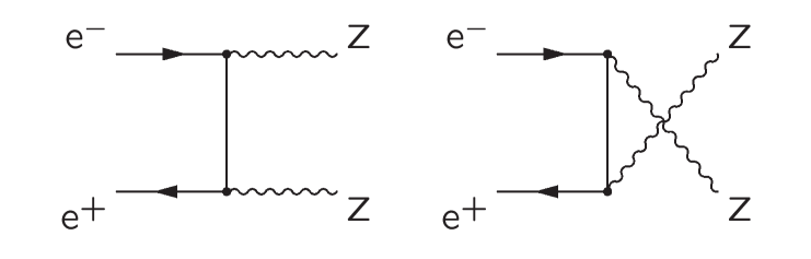
Figure 1: NC2 Feynman diagrams for the process $\mathrm{e^{+}}\mathrm{e^{-}}\to\mbox{$\mathrm{Z}$}\mbox{$\mathrm{Z}$}$ leading to a final state with four fermions.

The analyses and presentation of this paper largely follow that of the first OPAL $\mathrm{e^{+}}\mathrm{e^{-}}\to\mbox{$\mathrm{Z}$}\mbox{$\mathrm{Z}$}$ results at center-of-mass energies of 183 GeV and 189 GeV [3]. All of the analyses have been optimized for the higher energies and some adjustments to the analyses have been made to make them less sensitive to background.

This paper is organized as follows. In Section 2 we describe the data used and the Monte Carlo simulation of signal and background processes. In Section 3 we describe the selections for the processes ${\mbox{$\mathrm{Z}$}\mbox{$\mathrm{Z}$}\to{{\ell^{+}}{\ell^{-}}}{{\ell^{+}}{\ell^{-}}}}$, ${\mbox{$\mathrm{Z}$}\mbox{$\mathrm{Z}$}\to{\ell^{+}}{\ell^{-}}\nu\overline{\nu}}$, ${\mbox{$\mathrm{Z}$}\mbox{$\mathrm{Z}$}\to\mathrm{q}\overline{\mathrm{q}}\nu\overline{\nu}}$, ${\mbox{$\mathrm{Z}$}\mbox{$\mathrm{Z}$}\to\mathrm{q}\overline{\mathrm{q}}{\ell^{+}}{\ell^{-}}}$ and ${\mbox{$\mathrm{Z}$}\mbox{$\mathrm{Z}$}\to\mathrm{q}\overline{\mathrm{q}}\mathrm{q}\overline{\mathrm{q}}}$, where ${\ell^{+}}{\ell^{-}}$ denotes a charged lepton pair of opposite charge and $\mathrm{q}\overline{\mathrm{q}}$ any of the five lightest quark-antiquark pairs. We also consider the processes ${\mbox{$\mathrm{Z}$}\mbox{$\mathrm{Z}$}\to\mathrm{b}\overline{\mathrm{b}}{\ell^{+}}{\ell^{-}}}$, ${\mbox{$\mathrm{Z}$}\mbox{$\mathrm{Z}$}\to\mathrm{b}\overline{\mathrm{b}}\nu\overline{\nu}}$ and ${\mbox{$\mathrm{Z}$}\mbox{$\mathrm{Z}$}\to\mathrm{q}\overline{\mathrm{q}}\mathrm{b}\overline{\mathrm{b}}}$ using b-tagging methods similar to those developed for the OPAL Higgs search [10]. In Section 4 the selected events are used to measure the $\mathrm{Z}$-pair cross section. In this section we also test our measured values of the $\mathrm{Z}$-pair cross section and the value of the branching ratio BR$(\mbox{$\mathrm{Z}$}\to\mathrm{b}\overline{\mathrm{b}})$ measured in $\mathrm{Z}$-pair decays for consistency with the Standard Model prediction. At LEP, $\mathrm{Z}$-pair events with b quarks in the final state form the principle background to the search for Higgs bosons produced in association with a Z boson. In Section 5 anomalous neutral-current triple gauge couplings are constrained using the measured cross sections and kinematic variables combined in an optimal observables (OO) method. Finally, in Section 6 limits are placed on low scale gravity theories with large extra dimensions.

2 Data samples and Monte Carlo simulation

The OPAL detector, trigger and data acquisition system used for this study are described in References [11, 12, 15, 13, 14].

The approximate integrated luminosities and luminosity-weighted mean center-of-mass energies [16] for the data used in this analysis are given in Table 1. The actual integrated luminosities used for each final state vary due to differing detector status requirements. These luminosities were measured using small-angle Bhabha scattering events recorded in the silicon-tungsten luminometer [15, 17, 18] and the theoretical calculation given in Reference [19]. The overall uncertainty on the luminosity measurement amounts to less than 0.5% and contributes negligibly to our cross-section measurement error.

Energy point label	Mean center-of-mass energy	Approximate integrated luminosity
(GeV)	(GeV)	(pb-1)
192	$191.59\pm 0.04$	29
196	$195.53\pm 0.04$	73
200	$199.52\pm 0.04$	74
202	$201.63\pm 0.04$	37
205	$204.80\pm 0.05$	80
207	$206.53\pm 0.05$	140

Table 1: Luminosity-weighted mean center-of-mass energies and typical integrated luminosities for the data presented here. The integrated luminosities for each channel vary slightly since they depend on the status of different detector elements. The channel dependent luminosities are given in Tables 5 - 10.

Selection efficiencies and backgrounds were calculated using a simulation [20] of the OPAL detector. The simulated events were processed in the same manner as the data. We define the $\mathrm{Z}$$\mathrm{Z}$ cross section as the contribution to the total four-fermion cross section from the NC2 $\mathrm{Z}$-pair diagrams shown in Figure 1. All signal efficiencies given in this paper are with respect to these $\mathrm{Z}$-pair processes. Contributions from all other four-fermion final states, including interference with NC2 diagrams, are considered as background. For studies of the signal efficiency we have used grc4f [21] and YFSZZ [22] with PYTHIA [23] used for the parton shower and hadronization. YFSZZ only generates the NC2 diagrams. The grc4f Monte Carlo includes four-fermion background processes and the interference of background and the NC2 $\mathrm{Z}$$\mathrm{Z}$ signal. Weights, based on the grc4f matrix elements, are assigned to each grc4f Monte Carlo event for the event to originate from NC2 $\mathrm{Z}$$\mathrm{Z}$ signal, four-fermion background and interference between the four-fermion background and the NC2 $\mathrm{Z}$$\mathrm{Z}$ signal. In all of the fits performed in this analysis we use the ZZTO calculation [24] with the $G_{F}$ renormalization scheme for integrated Standard Model cross sections. To check the simulation of anomalous couplings in the YFSZZ Monte Carlo we use EEZZ [25].

Backgrounds are simulated using several different generators. KK2f [26] (with PYTHIA used for the parton shower and hadronization) is used to simulate two-fermion final states such as $\mathrm{e^{+}}\mathrm{e^{-}}\to\mbox{$\mathrm{Z}$}^{*}(n\gamma)\to\mathrm{q}\overline{\mathrm{q}}(n\gamma)$ and $\mathrm{e^{+}}\mathrm{e^{-}}\to\gamma^{*}(n\gamma)\to\mathrm{q}\overline{\mathrm{q}}(n\gamma)$, where $(n\gamma)$ indicates the generation of one or more initial-state radiated photons. HERWIG [27] and PYTHIA are used as checks for these final states. These two-fermion samples include gluon radiation from the quarks, which produce $\mathrm{q}\overline{\mathrm{q}}{\rm g}$, $\mathrm{q}\overline{\mathrm{q}}\mathrm{q}\overline{\mathrm{q}}$ and $\mathrm{q}\overline{\mathrm{q}}{\rm gg}$ final states. KK2f is also used to simulate muon and tau pair events and Bhabhas are modeled using BHWIDE [28] and TEEGG [29]. The grc4f generator, with the contribution exclusively due to NC2 diagrams removed, is used to simulate other four-fermion background. KORALW [30] and EXCALIBUR [31] are used as checks of the four-fermion background.

Multiperipheral (“two-photon”) processes with hadronic final states are simulated by combining events from PHOJET[32], for events without electrons scattered into the detector, and HERWIG [27], for events with single electrons scattered into the detector. Two-photon events with both the electron and positron scattered into the detector, which are only a signficant background for the $\mathrm{q}\overline{\mathrm{q}}\mathrm{e^{+}}\mathrm{e^{-}}$ final state, are simulated with TWOGEN [33]. The Vermaseren [34] generator is used to simulate multiperipheral production of the final states $\mathrm{e^{+}}\mathrm{e^{-}}{\ell^{+}}{\ell^{-}}$.

To avoid background from four-fermion final states mediated by a $\mathrm{Z}$ boson and a virtual $\gamma^{*}$, our selections were optimized on Monte Carlo samples to select events with candidate $\mathrm{Z}$-boson masses, $m_{1}$ and $m_{2}$, that satisfy $m_{1}+m_{2}>170\ \mathrm{GeV}$ and $|m_{1}-m_{2}|<20\ \mathrm{GeV}$. Above 190 GeV more than 90% of the events produced via the NC2 diagrams are contained in this mass region. Events from the NC2 diagrams dominate in this mass region except for final states containing electron pairs. However, inside the acceptance of the electromagnetic calorimeters, the backgrounds from two-photon and electroweak Compton scattering ($\mathrm{e}\gamma\to\mathrm{e}\mbox{$\mathrm{Z}$}$) processes [35] to $\mathrm{Z}$ final states with one $\mathrm{Z}$ decaying to electron pairs is reduced to less than 5% of the expected $\mathrm{Z}$-pair cross section and the NC2 diagrams again dominate.

3 Event selection

The OPAL selections cover all $\mathrm{Z}$$\mathrm{Z}$ final states except $\nu\overline{\nu}\nu\overline{\nu}$ and $\tau^{+}\tau^{-}\nu\overline{\nu}$. In hadronic final states, the energies and directions of the jets are determined using tracks to reconstruct charged particles and electromagnetic and hadronic calorimeter clusters to reconstruct neutral particles. The correction for unavoidable double counting due to the overlap of calorimeter energy deposited from charged and neutral particles is described in Reference [10].

In the $\mathrm{q}\overline{\mathrm{q}}\mathrm{e^{+}}\mathrm{e^{-}}$, $\mathrm{q}\overline{\mathrm{q}}\mu^{+}\mu^{-}$ and $\mathrm{q}\overline{\mathrm{q}}\mathrm{q}\overline{\mathrm{q}}$ analyses, four-constraint (4C) and five-constraint (5C) kinematic fits are used. The 4C fit imposes energy and momentum conservation. In the 5C fit the added constraint requires the masses of the two candidate $\mathrm{Z}$ bosons to be equal to one another. For final states with either $\mathrm{Z}$ boson decaying to a tau pair, the direction of each tau lepton is approximated by the reconstructed particles that identify the tau. The energies and total momenta of the tau leptons are obtained by leaving the reconstructed direction of the four fermions fixed and scaling the energy and momentum of each of the fermions to obtain energy and momentum conservation. The scaled values of the tau momentum and energy are then used in the subsequent steps of the analysis. In the $\mathrm{q}\overline{\mathrm{q}}\tau^{+}\tau^{-}$ final state, subsequent kinematic fits are therefore effectively 2C and 3C fits.

The selection procedures for events containing charged leptons or neutrinos (${\ell^{+}}{\ell^{-}}{\ell^{+}}{\ell^{-}}$,${\ell^{+}}{\ell^{-}}\nu\overline{\nu}$, $\mathrm{q}\overline{\mathrm{q}}{\ell^{+}}{\ell^{-}}$ and $\mathrm{q}\overline{\mathrm{q}}\nu\overline{\nu}$) are largely unchanged from the analysis used at 183 GeV and 189 GeV in Reference [3], except that the likelihood functions and some of the cuts have been optimized for the higher energies. More significant changes have been made to the $\mathrm{q}\overline{\mathrm{q}}\mathrm{q}\overline{\mathrm{q}}$ and $\mathrm{q}\overline{\mathrm{q}}\mathrm{b}\overline{\mathrm{b}}$ selections.

3.1 Selection of ${\mbox{$\mathrm{Z}$}\mbox{$\mathrm{Z}$}\to{{\ell^{+}}{\ell^{-}}}{{\ell^{+}}{\ell^{-}}}}$ events

$\mathrm{Z}$-pairs decaying to final states with four charged leptons (${\ell^{+}}{\ell^{-}}{\ell^{+}}{\ell^{-}}$) produce low multiplicity events with a clear topological signature that is exploited to maximize the selection efficiency. The ${\ell^{+}}{\ell^{-}}{\ell^{+}}{\ell^{-}}$ analysis begins by selecting low multiplicity events (less than 13 reconstructed good tracks and less than 13 electromagnetic clusters) with visible energy of at least $0.2\sqrt{s}$ and at least one good track with momentum of 5 GeV or more. Good tracks are required to be consistent with originating from the interaction point and to be composed of space points from at least half of the maximum possible number of central tracking detector (Jet Chamber) sense wires.

Using a cone algorithm, the events are required to have exactly four cones of $15^{\circ}$ half angle each containing between 1 and 3 tracks. Cones of opposite charge are paired to form $\mathrm{Z}$ boson candidates.

Lepton identification is only used to classify events as background or to reduce the number of cone combinations considered by preventing the matching of identified electrons with identified muons. Electrons are identified on the basis of energy deposition in the electromagnetic calorimeter, track curvature and specific ionization in the tracking chambers. Muons are identified using the association between tracks and hits in the hadron calorimeter and muon chambers.

To reduce background from two-photon events with a single scattered electron detected, we eliminate events with forward-going electrons or backward-going positrons with the cuts $\cos\theta_{\mathrm{e^{-}}}<0.85$ and $\cos\theta_{\mathrm{e^{+}}}>-0.85$. Here $\theta_{\mathrm{e^{-}}}$ ( $\theta_{\mathrm{e^{+}}}$) is the angle of the electron (positron) with respect to the incoming electron beam. Background from partially reconstructed $\mathrm{q}\overline{\mathrm{q}}(n\gamma)$ events and two-photon events is reduced by requiring that most of the energy not be concentrated in a single cone. Defining $E_{\mathrm{vis}}$ as the total visible energy of the event and $E_{\mathrm{cone}}^{\mathrm{max}}$ as the energy contained in the most energetic cone we require $E_{\mathrm{vis}}-E_{\mathrm{cone}}^{\mathrm{max}}>0.2\sqrt{s}$.

The invariant masses of the lepton pairs are calculated in three different ways which are motivated by the possibility of having zero, one or two tau pairs in the event. The events are first classified according to the assumed number of tau pairs in the event:

1. Events without tau pairs can be selected by requiring a high visible energy. Therefore, events with $\mbox{$E_{\mathrm{vis}}$}>0.9\sqrt{s}$ are treated as $\mathrm{e^{+}}\mathrm{e^{-}}\mathrm{e^{+}}\mathrm{e^{-}}$, $\mathrm{e^{+}}\mathrm{e^{-}}\mu^{+}\mu^{-}$ or $\mu^{+}\mu^{-}\mu^{+}\mu^{-}$ events. We also treat all events with $|\cos\theta_{\mathrm{miss}}|>0.98$ ($\theta_{\mathrm{miss}}$ is the polar angle associated with the missing momentum in the event) as $\mathrm{e^{+}}\mathrm{e^{-}}\mathrm{e^{+}}\mathrm{e^{-}}$, $\mathrm{e^{+}}\mathrm{e^{-}}\mu^{+}\mu^{-}$ or $\mu^{+}\mu^{-}\mu^{+}\mu^{-}$ events to maintain efficiency for $\mathrm{Z}$-pairs with initial-state radiation. As there are no missing neutrinos in these events, the mass of each cone-pair combination is evaluated using the measured energies and momenta of the leptons.

2. Events failing (1) with a cone-pair combination that has energy exceeding $0.9m_{\smash{\mathrm{Z}}\mathstrut}$ are tried as an $\mathrm{e^{+}}\mathrm{e^{-}}\tau^{+}\tau^{-}$ or $\mu^{+}\mu^{-}\tau^{+}\tau^{-}$ final state. The mass of the tau-pair system is calculated from the recoil mass of the presumed electron or muon pair.

3. Events failing (1) with a cone-pair combination failing (2) are treated as $\tau^{+}\tau^{-}\tau^{+}\tau^{-}$ final states. The momenta of the tau leptons are determined using the scaling procedure described in the introduction to Section 3. The invariant masses of the cone pairs are evaluated using the scaled momenta.

In any event where the lepton identification allows more than one valid combination, each combination is tested using invariant mass cuts. For events with one or more combinations of cone-pairings satisfying $|m_{\smash{\mathrm{Z}}\mathstrut}-m_{\ell\ell}|<0.1m_{\smash{\mathrm{Z}}\mathstrut}$ and $|m_{\smash{\mathrm{Z}}\mathstrut}-m_{\ell^{\prime}\ell^{\prime}}|<0.1m_{\smash{\mathrm{Z}}\mathstrut}$ the one with the smallest value of $(m_{\smash{\mathrm{Z}}\mathstrut}-m_{\ell\ell})^{2}+(m_{\smash{\mathrm{Z}}\mathstrut}-m_{\ell^{\prime}\ell^{\prime}})^{2}$ is selected for further analysis. In the other events, the combination with the smallest value of $|m_{\smash{\mathrm{Z}}\mathstrut}-m_{\ell\ell}|$ or $|m_{\smash{\mathrm{Z}}\mathstrut}-m_{\ell^{\prime}\ell^{\prime}}|$ is selected. These requirements maintain efficiency for signal events with a single off-shell $\mathrm{Z}$ boson. The final event sample is then chosen with the requirement $m_{\ell\ell}+m_{\ell^{\prime}\ell^{\prime}}>160$ GeV and $|m_{\ell\ell}-m_{\ell^{\prime}\ell^{\prime}}|<40$ GeV. The signal detection efficiency, averaged over all ${\ell^{+}}{\ell^{-}}{\ell^{+}}{\ell^{-}}$ final states is approximately 56%. The efficiency for individual final states ranges from about 30% for $\tau^{+}\tau^{-}\tau^{+}\tau^{-}$ to more than 70% for $\mu^{+}\mu^{-}\mu^{+}\mu^{-}$. These efficiencies have almost no dependence on center-of-mass energy. In Table 2 (line a) we give the efficiency, background and observed number of events. The errors on the efficiency and background include the systematic uncertainties which are discussed in Section 3.6. The invariant masses of all cone pairs passing one of the selections are shown in Figure 2a. A total of four ${\ell^{+}}{\ell^{-}}{\ell^{+}}{\ell^{-}}$ events is observed between 190 GeV and 209 GeV with an expected background of $1.08\pm 0.27$ events. The remaining background is dominated by four-lepton events which are not from the NC2 diagrams that define $\mathrm{Z}$-pair production.

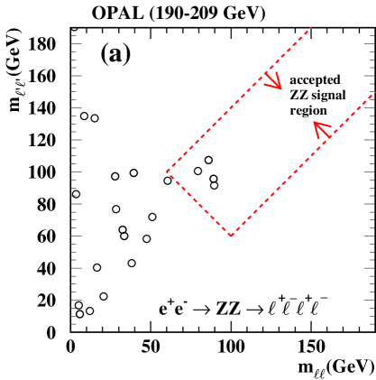
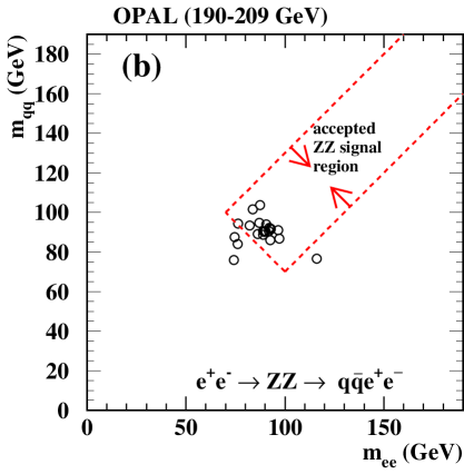
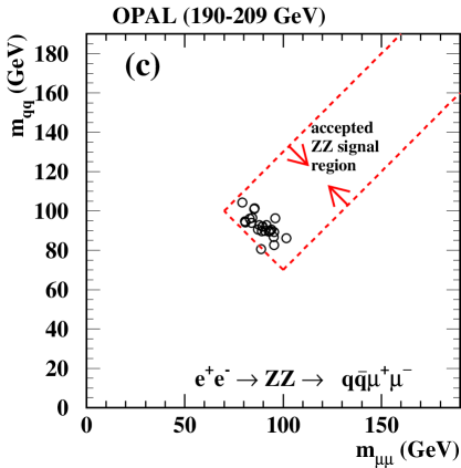
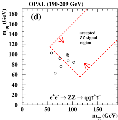
Figure 2: (a) Invariant masses of ${\ell^{+}}{\ell^{-}}{\ell^{+}}{\ell^{-}}$ cone pairs. Invariant mass pairs for the (b) $\mathrm{q}\overline{\mathrm{q}}\mathrm{e^{+}}\mathrm{e^{-}}$ (c) $\mathrm{q}\overline{\mathrm{q}}\mu^{+}\mu^{-}$ and (d) $\mathrm{q}\overline{\mathrm{q}}\tau^{+}\tau^{-}$ data. The dashed lines show the final invariant mass cuts. In contrast to Reference [3], the $\mathrm{q}\overline{\mathrm{q}}\mathrm{e^{+}}\mathrm{e^{-}}$, $\mathrm{q}\overline{\mathrm{q}}\mu^{+}\mu^{-}$ unconstrained invariant masses are plotted after the requirement that the 5C fit mass, with both quark and lepton-pair masses constrained to be the same, exceeds 85 GeV. The $\mathrm{q}\overline{\mathrm{q}}\tau^{+}\tau^{-}$ unconstrained invariant masses are shown after a similar cut on the 3C fit mass.

3.2 Selection of ${\mbox{$\mathrm{Z}$}\mbox{$\mathrm{Z}$}\to{\ell^{+}}{\ell^{-}}\nu\overline{\nu}}$ events

The selection of the $\mathrm{e^{+}}\mathrm{e^{-}}\nu\overline{\nu}$ and $\mu^{+}\mu^{-}\nu\overline{\nu}$ final states is based on the OPAL selection of $\mathrm{W}$ pairs decaying to leptons [36]. The mass and momentum of the $\mathrm{Z}$ boson decaying to $\nu\overline{\nu}$ are calculated using the beam-energy constraint and the reconstructed energy and momentum of the $\mathrm{Z}$ boson decaying to a charged lepton pair. A likelihood selection based on the visible and recoil masses as well as the polar angle of the leptons, is then used to separate signal from background.

The $\mathrm{e^{+}}\mathrm{e^{-}}\nu\overline{\nu}$ selection starts with OPAL $\mathrm{W}$-pair candidates where both charged leptons are classified as electrons. Each event is then divided into two hemispheres using the thrust axis. In each hemisphere, the track with the highest momentum is selected as the leading track. The sum of the charges of these two tracks is required to be zero. The determination of the visible mass, $m_{\mathrm{vis}}$, and the recoil mass, $m_{\mathrm{recoil}}$, is based on the energy as measured in the electromagnetic calorimeter and the direction of the leading tracks.

The likelihood selection uses three variables: $Q\cos\theta$, where $\theta$ is the angle of the track with the highest momentum and $Q$ is its charge, the normalized sum of visible and recoil masses $(m_{\mathrm{vis}}+m_{\mathrm{recoil}})/\sqrt{s}$ and the difference of visible and recoil masses, $m_{\mathrm{vis}}-m_{\mathrm{recoil}}$. The performance of the likelihood selection is improved with the following preselection: $\mathrm{-25\,GeV}<m_{\mathrm{vis}}-m_{\mathrm{recoil}}<\mathrm{15\,GeV}$ and $(m_{\mathrm{vis}}+m_{\mathrm{recoil}})>170$ GeV. Two events with ${\cal L}_{\mathrm{e^{+}}\mathrm{e^{-}}\nu\overline{\nu}}>0.60$ are selected. See Table 2 (line b) and Figure 3a. The expected background is primarily from $\mathrm{W}$ pairs and amounts to $1.28\pm 0.15$ events.

The $\mu^{+}\mu^{-}\nu\overline{\nu}$ selection starts with the OPAL $\mathrm{W}$-pair candidates where both charged leptons are classified as muons. The selection procedure is the same as for the $\mathrm{e^{+}}\mathrm{e^{-}}\nu\overline{\nu}$ final states except that $m_{\mathrm{vis}}$ and $m_{\mathrm{recoil}}$ are calculated from the momentum of the reconstructed tracks of the $\mathrm{Z}$ boson decaying to muon pairs. The likelihood preselections $\mathrm{-25\,GeV}<m_{\mathrm{vis}}-m_{\mathrm{recoil}}<\mathrm{25\,GeV}$ and $(m_{\mathrm{vis}}+m_{\mathrm{recoil}})>170$ GeV are applied. No event with ${\cal L}_{\mu^{+}\mu^{-}\nu\overline{\nu}}>0.60$ is selected while $4.30\pm 0.39$ are expected (see Table 2 (line c) and Figure 3b). The probability to observe no event when $4.3\pm 0.39$ are expected is approximately 1.4%.

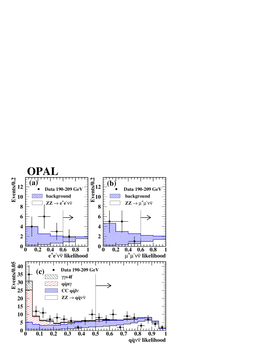
Figure 3: Likelihood discriminant used at $\sqrt{s}>190$ GeV for (a) the $\mathrm{e^{+}}\mathrm{e^{-}}\nu\overline{\nu}$ selection, (b) the $\mu^{+}\mu^{-}\nu\overline{\nu}$ selection and the (c) the $\mathrm{q}\overline{\mathrm{q}}\nu\overline{\nu}$ selection. The dotted line and arrow show the position of the likelihood cut used to select ZZ events in each case.

3.3 Selection of ${\mbox{$\mathrm{Z}$}\mbox{$\mathrm{Z}$}\to\mathrm{q}\overline{\mathrm{q}}{\ell^{+}}{\ell^{-}}}$ events

The lepton pairs in the $\mathrm{q}\overline{\mathrm{q}}\mathrm{e^{+}}\mathrm{e^{-}}$ and $\mathrm{q}\overline{\mathrm{q}}\mathrm{\mu^{+}}\mathrm{\mu^{-}}$ final states have a distinctive signature making possible selections with high efficiencies and low background contaminations. In the $\mathrm{q}\overline{\mathrm{q}}\tau^{+}\tau^{-}$ final state, the decay of the tau leptons produces events which are more difficult to identify. The identification of this final state exploits the missing momentum and missing energy carried away by the neutrinos produced in the decay of the tau lepton. In comparison to our previous publication [3], the $\mathrm{q}\overline{\mathrm{q}}\mathrm{e^{+}}\mathrm{e^{-}}$ and $\mathrm{q}\overline{\mathrm{q}}\mathrm{\mu^{+}}\mathrm{\mu^{-}}$ selections are almost unchanged, but the analysis of $\mathrm{q}\overline{\mathrm{q}}\tau^{+}\tau^{-}$ events with b-tags has been simplified. The $\mathrm{q}\overline{\mathrm{q}}\mathrm{e^{+}}\mathrm{e^{-}}$ and $\mathrm{q}\overline{\mathrm{q}}\mu^{+}\mu^{-}$ selections presented here are also similar to those used in [37] but are optimized specifically for $\mathrm{Z}$-pair final states.

3.3.1 Selection of ${\mbox{$\mathrm{Z}$}\mbox{$\mathrm{Z}$}\to\mathrm{q}\overline{\mathrm{q}}\mathrm{e^{+}}\mathrm{e^{-}}}$ and ${\mbox{$\mathrm{Z}$}\mbox{$\mathrm{Z}$}\to\mathrm{q}\overline{\mathrm{q}}\mu^{+}\mu^{-}}$ events

The selection of $\mathrm{q}\overline{\mathrm{q}}\mathrm{e^{+}}\mathrm{e^{-}}$ and $\mathrm{q}\overline{\mathrm{q}}\mu^{+}\mu^{-}$ final states requires the visible energy of the events to be greater than 90 GeV and at least six reconstructed tracks. Among all tracks with momenta greater than 2 GeV, the highest momentum track is taken as the first lepton candidate and the second-highest momentum track with a charge opposite to the first candidate is taken as the second lepton candidate. Using the Durham [38] jet algorithm, the event, including the lepton candidates, is forced into four jets and the jet resolution variable that separates the three-jet topology from the four-jet topology, $y_{34}$, is required to be greater than $10^{-3}$. Excluding the electron or muon candidates and their associated calorimeter clusters, the rest of the event is forced into two jets. The 4C and 5C fits to the two lepton candidates and the two jets are required to converge.

In the $\mathrm{q}\overline{\mathrm{q}}\mathrm{e^{+}}\mathrm{e^{-}}$ selection no explicit electron identification is used. Electron candidates are selected by requiring the sum of the electromagnetic cluster energies $E_{1}+E_{2}$ associated to the electrons to be greater than 70 GeV and the momentum of the track associated with the most energetic electron candidate to exceed 20 GeV. We also reject the event if the angle between either electron candidate and any other track is less than 5^∘.

In the $\mathrm{q}\overline{\mathrm{q}}\mu^{+}\mu^{-}$ selection the muons are identified using (i) tracks which match a reconstructed segment in the muon chambers, (ii) tracks which are associated to hits in the hadron calorimeter or muon chambers [36], or (iii) isolated tracks associated to electromagnetic clusters with reconstructed energy less than 2 GeV. No isolation requirement is imposed on events with both muon tracks passing (i) or (ii). Events with at least one muon identified with criterion (iii) are accepted if both muon candidates in the event have an angle of at least 10^∘ to the nearest track. We require the sum of the momenta of the two leptons to be greater than 70 GeV.

$\mathrm{Z}$-pair events are separated from $\mbox{$\mathrm{Z}$}\gamma^{*}$ background by requiring the fitted mass of the 5C fit to be larger than 85 GeV and the invariant masses $m_{\ell\ell}$ and $m_{\mathrm{qq}}$ obtained from the 4C fit to satisfy $(m_{\ell\ell}+m_{\mathrm{qq}})>170$ GeV and $|m_{\ell\ell}-m_{\mathrm{qq}}|<30$ GeV. Figure 2b (2c) shows the distribution of $m_{\rm ee}$ ($m_{\mu\mu}$) and $m_{\mathrm{qq}}$ before the cuts on the masses from the 4C fit.

After all cuts the mean selection efficiency for $\mathrm{q}\overline{\mathrm{q}}\mathrm{e^{+}}\mathrm{e^{-}}$ signal events is 60% and depends weakly on energy. A total of 17 candidate events is found after all cuts at $\sqrt{s}$ between 190 GeV and 209 GeV, which can be compared to the Standard Model expectation (including a small background) of $14.1\pm 0.4$. In Table 2 (lines d and e) we give the efficiency, background and observed number of events. The errors on these efficiencies and backgrounds include the systematic uncertainties (see Section 3.6). The largest source of background after all cuts is from the process $\mathrm{e^{+}}\mathrm{e^{-}}\to\mbox{$\mathrm{Z}$}\gamma^{*}\to\mathrm{q}\overline{\mathrm{q}}\mathrm{e^{+}}\mathrm{e^{-}}$ and from two-photon events.

In the $\mathrm{q}\overline{\mathrm{q}}\mu^{+}\mu^{-}$ selection, the mean selection efficiency is 73% and varies less than 5% with energy. A total of 22 events is observed at $\sqrt{s}$ between 190 GeV and 209 GeV, which can be compared to the Standard Model expectation (including a small background) of $15.5\pm 0.4$. (See Table 2 lines f and g). The background after all cuts is expected to come mainly from $\mathrm{e^{+}}\mathrm{e^{-}}\to\mbox{$\mathrm{Z}$}\gamma^{*}\to\mathrm{q}\overline{\mathrm{q}}\mu^{+}\mu^{-}$ events.

3.3.2 Selection of $\mathrm{e^{+}}\mathrm{e^{-}}\to\mbox{$\mathrm{Z}$}\mbox{$\mathrm{Z}$}\to\mathrm{q}\overline{\mathrm{q}}\tau^{+}\tau^{-}$ events

The $\mathrm{q}\overline{\mathrm{q}}\tau^{+}\tau^{-}$ final state is selected from a sample of events with track multiplicity greater than or equal to six. Events which pass all the requirements of the $\mathrm{q}\overline{\mathrm{q}}\mathrm{e^{+}}\mathrm{e^{-}}$ and $\mathrm{q}\overline{\mathrm{q}}\mu^{+}\mu^{-}$ selections are excluded from this selection. The tau-lepton candidates are selected using a neural network algorithm which is described in detail in Reference [10]. At least two tau candidates are required. The tau candidate with the highest neural network output value is taken as the first candidate. The second candidate is required to have its charge opposite to the first candidate and the highest neural network output value among all remaining candidates.

Because of the presence of neutrinos in the final state the missing energy, $\sqrt{s}-E_{\mathrm{vis}}$, is required to exceed 15 GeV while the visible energy of the event, $E_{\mathrm{vis}}$, is required to exceed 90 GeV. In addition, the sum of the momenta of the leading tracks from the tau-lepton decays is required to be less than 70 GeV. Since the direction of the missing momentum in signal events will tend to be along the direction of one of the decaying tau leptons, the angle $\alpha_{\tau,{\rm miss}}$ between the missing momentum and a tau-lepton candidate is required to satisfy $\alpha_{\tau,{\rm miss}}<90^{\circ}$ for at least one of the two tau candidates.

The two hadronic jets are selected in the same way as in the $\mathrm{e^{+}}\mathrm{e^{-}}\to\mbox{$\mathrm{Z}$}\mbox{$\mathrm{Z}$}\to\mathrm{q}\overline{\mathrm{q}}\mathrm{e^{+}}\mathrm{e^{-}}$ selection. The initial estimate of the energy and the momenta of the tau candidates is found from the sum of the momenta of the tracks associated to the tau by the neural network algorithm and all unassociated electromagnetic clusters in a cone with a half angle of 10^∘ around the leading track from the tau decay. A 2C kinematic fit that imposes energy and momentum conservation (see the introduction to Section 3) is required to converge. A 3C kinematic fit, with the additional constraint of the equality of the fermion pair masses is also required to converge.

Using the network output [10] for each tau candidate, a tau lepton probability, ${\cal P}$, is calculated taking into account the different branching ratios, sensitivities, efficiencies and background levels for 1-prong and 3-prong tau-lepton decays. In this paper, we combine two probabilities ${\cal P}_{1}$ and ${\cal P}_{2}$, to form a likelihood ratio using

$${\cal L}=\frac{{\cal P}_{1}{\cal P}_{2}}{{\cal P}_{1}{\cal P}_{2}+(1-{\cal P}_{1})(1-{\cal P}_{2})}.$$ (1)

The likelihood ratio associated with probabilities of the two tau candidates is required to satisfy ${\cal L}_{\tau\tau}>0.977$. In addition, the common mass of the 3C fit is required to exceed 85 GeV. Using the 2C fit masses of the tau pair, $m_{\smash{\mathrm{\tau\tau}}\mathstrut}$, and the quark pair, $m_{\mathrm{qq}}$, as obtained from the kinematic fit, we also require $m_{\mathrm{qq}}+m_{\smash{\mathrm{\tau\tau}}\mathstrut}>170$ GeV and $|m_{\mathrm{qq}}-m_{\smash{\mathrm{\tau\tau}}\mathstrut}|<60$ GeV.

Four candidate events are found in the data. Figure 2d shows the masses of the candidate events before the invariant mass cuts. In Table 2 (lines h and i) we give the efficiencies, backgrounds and observed number of events.

3.3.3 Selection of $\mathrm{e^{+}}\mathrm{e^{-}}\to\mbox{$\mathrm{Z}$}\mbox{$\mathrm{Z}$}\to\mathrm{b}\overline{\mathrm{b}}{\ell^{+}}{\ell^{-}}$

The selection of the $\mathrm{b}\overline{\mathrm{b}}{\ell^{+}}{\ell^{-}}$ events is based on the $\mathrm{q}\overline{\mathrm{q}}{\ell^{+}}{\ell^{-}}$ selections with addition of the algorithm described in Reference [10] to identify $\mathrm{b}\overline{\mathrm{b}}$ final states. The probabilities that each of the hadronic jets is a b jet can be combined to form a likelihood function, ${\cal L}_{\mathrm{bb}}$, according to Equation (1). Because the $\mathrm{q}\overline{\mathrm{q}}\mathrm{e^{+}}\mathrm{e^{-}}$ and $\mathrm{q}\overline{\mathrm{q}}\mu^{+}\mu^{-}$ selections are pure, a relatively loose cut of ${\cal L}_{\mathrm{bb}}>0.2$ is used to select the $\mathrm{b}\overline{\mathrm{b}}\mathrm{e^{+}}\mathrm{e^{-}}$ and $\mathrm{b}\overline{\mathrm{b}}\mu^{+}\mu^{-}$ samples. For the selections with electron and muon pairs there are two classes of events since the selected $\mathrm{b}\overline{\mathrm{b}}{\ell^{+}}{\ell^{-}}$ events are a subset of the $\mathrm{q}\overline{\mathrm{q}}{\ell^{+}}{\ell^{-}}$ events. In Table 2 (lines e and g) we give the efficiencies of the b-tagged samples with respect to the expected fraction of $\mathrm{b}\overline{\mathrm{b}}$ events. The efficiencies for samples without b-tags are given with respect to the hadronic decays without $\mathrm{b}\overline{\mathrm{b}}$ final states.

In the data with $\sqrt{s}$ above 190 GeV we find three candidate $\mathrm{b}\overline{\mathrm{b}}\mathrm{e^{+}}\mathrm{e^{-}}$ events with $2.49\pm 0.19$ expected and in the $\mathrm{b}\overline{\mathrm{b}}\mu^{+}\mu^{-}$ selection we find seven events with $2.59\pm 0.15$ events expected. The probability to observe seven or more events when $2.59\pm 0.15$ are expected is approximately 1.7%. The invariant masses of these seven events are consistent with $m_{\mathrm{Z}}$.

For the $\mathrm{b}\overline{\mathrm{b}}\tau^{+}\tau^{-}$ selection the ${\cal L}_{\mathrm{\tau\tau}}$ cut of the $\mathrm{q}\overline{\mathrm{q}}\tau^{+}\tau^{-}$ selection is loosened and combined with ${\cal L}_{\mathrm{bb}}$ as follows. ${\cal L}_{\tau\tau}$ and ${\cal L}_{\mathrm{bb}}$ are both required to be greater than 0.1. The $\mathrm{b}\overline{\mathrm{b}}\tau^{+}\tau^{-}$ probability for the event, ${\cal L}_{\mathrm{bb}\tau\tau}$, is calculated from Equation (1) with ${\cal L}_{\tau\tau}$ and ${\cal L}_{\mathrm{bb}}$ as inputs and required to exceed 0.95. After the cut on ${\cal L}_{\mathrm{bb}\tau\tau}$, the remaining cuts of the $\mathrm{q}\overline{\mathrm{q}}\tau^{+}\tau^{-}$ selection are applied. None of the $\mathrm{q}\overline{\mathrm{q}}\tau^{+}\tau^{-}$ events are identified as $\mathrm{b}\overline{\mathrm{b}}\tau^{+}\tau^{-}$ candidates which can be compared with the Standard Model expectation of $1.41\pm 0.19$. One additional candidate event is found in the sample with the relaxed cut on ${\cal L}_{\mathrm{\tau\tau}}$ with $0.35\pm 0.10$ expected. See Table 2 (lines i and j).

3.4 Selection of ${\mbox{$\mathrm{Z}$}\mbox{$\mathrm{Z}$}\to\mathrm{q}\overline{\mathrm{q}}\nu\overline{\nu}}$ events

The $\mathrm{q}\overline{\mathrm{q}}\nu\overline{\nu}$ selection is based on the reconstruction of the $\mathrm{Z}$ boson decaying to $\mathrm{q}\overline{\mathrm{q}}$ which produces slightly boosted back-to-back jets. The selection uses events with a two-jet topology where both jets are contained in the detector. The beam energy constraint is used to determine the mass of the $\mathrm{Z}$ boson decaying to $\nu\overline{\nu}$. The properties of the $\mathrm{q}\overline{\mathrm{q}}$ decay and the inferred mass of the $\nu\overline{\nu}$ decay are then used in a likelihood analysis to separate signal from background.

Two-jet events are selected by dividing each event into two hemispheres using the plane perpendicular to the thrust axis. The number of tracks in each hemisphere is required to be four or more. The polar angles of the energy-momentum vector associated with each hemisphere, $\theta_{\mathrm{hemi1}}$ and $\theta_{\mathrm{hemi2}}$, are used to define the quantity ${\cos\theta_{\mathrm{h}}}\equiv\frac{1}{2}(\cos\theta_{\mathrm{hemi1}}-\cos\theta_{\mathrm{hemi2}})$. Contained events are selected by requiring $|{\cos\theta_{\mathrm{h}}}|<0.80$. The total energy in the forward detectors and in the forward region of the electromagnetic calorimeter ($|\cos\theta|>0.95$) is required to be less than 3 GeV. $\mathrm{W}$ boson decays identified by the OPAL $\mathrm{W}$-pair selection are rejected using the likelihood function for $\mathrm{e^{+}}\mathrm{e^{-}}\to\mathrm{\mathrm{q}\overline{\mathrm{q}}}\ell\nu$ from Reference [36] which includes an optimization for each center-of-mass energy. Only events with ${\cal L}_{\mathrm{W}\mathrm{W}}<0.5$ are retained.

An important background to our selection is $\mathrm{q}\overline{\mathrm{q}}(n\gamma)$ events with photons that escape detection. We discriminate against these events by looking for a significant amount of missing transverse momentum, $p_{\mathrm{t}}$. In each event, $p_{\mathrm{t}}$ can be resolved into two components, $p_{\mathrm{t}i}$, perpendicular to the transverse component of the thrust axis and $p_{\mathrm{t}j}$, along the transverse component of the thrust axis. $p_{\mathrm{t}i}$ depends primarily on the reconstructed angles of the jets and therefore is more precisely measured than $p_{\mathrm{t}j}$ which depends on the energy balance of the jets. We approximate $p_{\mathrm{t}i}$ as $p_{\mathrm{t}i}=\frac{1}{2}E_{\mathrm{b}}\sin\phi\sin\theta_{\mathrm{h}}$. Here $E_{\mathrm{b}}=\sqrt{s}/2$ is the beam energy, $\phi$ is the acoplanarity calculated from the angle between the transverse components of the momentum vectors of the two hemispheres and $\sin\theta_{\mathrm{h}}=\sqrt{1-\cos^{2}\theta_{\mathrm{h}}}$. The resolution on $p_{\mathrm{t}i}$, $\sigma_{p_{\mathrm{t}i}}$, was parameterized as a function of thrust and ${\cos\theta_{\mathrm{h}}}$ using data taken at the $\mathrm{Z}$ resonance. We construct the variable

$$R_{p_{\mathrm{t}i}}=(p_{\mathrm{t}i}-p_{\mathrm{t}i}^{0})/\sigma_{p_{\mathrm{t}i}},$$ (2)

which is used as input to the likelihood function described below. Here $p_{\mathrm{t}i}^{0}$ corresponds to the transverse momentum carried by a photon with half the beam energy which just misses the inner edge of our acceptance ( $p_{\mathrm{t}i}^{0}=E_{\mathrm{b}}\sin(32\,\mbox{mrad})/2$). The likelihood function also uses the related variable $\cos\theta_{\mathrm{miss}}$, the direction of the missing momentum in the event, to discriminate against the $\mathrm{q}\overline{\mathrm{q}}(n\gamma)$ events.

In the final selection of events, we use a likelihood function based on the following five variables:

1. the normalized sum of visible and recoil masses $(m_{\mathrm{vis}}+m_{\mathrm{recoil}})/\sqrt{s}$,

2. the difference of visible and recoil masses ($m_{\mathrm{vis}}-m_{\mathrm{recoil}}$),

3. $\log(y_{23})$, where $y_{23}$ is the jet resolution parameter that separates the two-jet topology from the three-jet topology as calculated from the Durham jet algorithm,

4. $\cos\theta_{\mathrm{miss}}$ and

5. $R_{p_{\mathrm{t}i}}$.

The mass variables are useful for reducing background from $\mathrm{W}$-pair production and single $\mathrm{W}$ ($\mathrm{W}\mathrm{e}\nu$) final states. The jet resolution parameter is useful in reducing the remaining $\mathrm{\mathrm{q}\overline{\mathrm{q}}}\ell\nu$ final states. To improve the performance of the likelihood analysis we use only events with $|m_{\mathrm{vis}}-m_{\mathrm{recoil}}|<50$ GeV, $(m_{\mathrm{vis}}+m_{\mathrm{recoil}})>170$ GeV and $R_{p_{\mathrm{t}i}}>1.2$. Events are then selected using ${\cal L}_{\mathrm{q}\overline{\mathrm{q}}\nu\overline{\nu}}>0.5$, where ${\cal L}_{\mathrm{q}\overline{\mathrm{q}}\nu\overline{\nu}}$ is the likelihood function for the $\mathrm{q}\overline{\mathrm{q}}\nu\overline{\nu}$ selection. The likelihood distribution of data and Monte Carlo simulation is shown in Figure 3c. For the $\mathrm{b}\overline{\mathrm{b}}\nu\overline{\nu}$ selection we require, in addition, the b-tag variable of Reference [10] to be greater than 0.65.

The mean efficiency for the $\mathrm{q}\overline{\mathrm{q}}\nu\overline{\nu}$ selection alone is $32\%$ and does not have a strong dependence on $\sqrt{s}$. The efficiency includes corrections to the Monte Carlo simulation for the effects of backgrounds in the foward detectors and for imperfect detector modeling. The modeling systematic uncertainties are discussed below in Section 3.6. A total of 60 candidates is observed in the data to be compared with the Standard Model expectation of $64.9\pm 2.9$. The efficiencies after considering the results of the b-tagging, as well as the number of events selected are given in Table 2 (lines k and l).

3.5 Selection of ${\mbox{$\mathrm{Z}$}\mbox{$\mathrm{Z}$}\to\mathrm{q}\overline{\mathrm{q}}\mathrm{q}\overline{\mathrm{q}}}$ events

As in the previous analysis [3] the hadronic selection consists of a preselection followed by two different likelihood selections, one of them aiming at an inclusive selection of fully hadronic $\mathrm{Z}$-pair decays, and the other optimized for selecting final states containing at least one pair of b quarks. The main changes with respect to the previous analysis are that cuts in the preselection have been modified slightly and that the quantities used in the $\mathrm{q}\overline{\mathrm{q}}\mathrm{b}\overline{\mathrm{b}}$ likelihood have changed.

3.5.1 Preselection

The preselection starts from the inclusive multihadron selection described in Reference [17]. The radiative process $\mathrm{e^{+}}\mathrm{e^{-}}\to\mbox{$\mathrm{Z}$}\gamma\to\mathrm{q}\overline{\mathrm{q}}\gamma$ is suppressed by requiring the effective center-of-mass energy after initial-state radiation, $\sqrt{s^{\prime}}$, to be larger than 160 GeV. $\sqrt{s^{\prime}}$ is obtained from a kinematic fit [17] that allows for one or more radiative photons in the detector or along the beam pipe. The final-state particles are then grouped into jets using the Durham algorithm [38]. A four-jet sample is formed by requiring the jet resolution parameter $y_{34}$ to be at least $0.003$ and each jet to contain at least two tracks. In order to suppress $\mbox{$\mathrm{Z}$}^{*}/\gamma^{*}\to\mathrm{q}\overline{\mathrm{q}}$ background, the event shape parameter $C_{\mathrm{par}}$ [39], which is large for spherical events, is required to be greater than 0.27. A 4C kinematic fit using energy and momentum conservation is required to converge. A 5C kinematic fit which forces the two jet pairs to have the same mass is applied in turn to all three possible combinations of the four jets. This fit is required to converge for at least one combination.

The most probable pairing of the jets is determined using a likelihood discriminant which is based on the difference between the two di-jet masses calculated from the results of a 4C kinematic fit, the di-jet mass obtained from a 5C kinematic fit, and the $\chi^{2}$ probability of the 5C fit.

3.5.2 Likelihood for the inclusive $\mbox{$\mathrm{Z}$}\mbox{$\mathrm{Z}$}\to\mathrm{q}\overline{\mathrm{q}}\mathrm{q}\overline{\mathrm{q}}$ event selection

We use a likelihood selection with six input variables for the selection of $\mbox{$\mathrm{Z}$}\mbox{$\mathrm{Z}$}\to\mathrm{q}\overline{\mathrm{q}}\mathrm{q}\overline{\mathrm{q}}$ events. The likelihood selection is optimized separately for each energy point. The first variable is the output value of the jet pairing likelihood described above. The second variable is determined by excluding the jet pairing with the largest difference between the two di-jet masses as obtained from the 4C fit, and then evaluating the 5C-fit masses of the remaining two pairings. The one which is closest to the $\mathrm{W}$ mass is selected and the difference between this 5C-fit mass and the $\mathrm{W}$ mass is used in order to discriminate against hadronic $\mathrm{W}$-pair events. The third variable suppresses background events with radiated photons that shift the value of the mass obtained from the kinematic fit. We use the value of $\sqrt{s^{\prime}}$ from the preselection. The fourth variable is used to discriminate against $\mbox{$\mathrm{Z}$}^{*}/\gamma^{*}$ events. We use the difference between the largest and smallest jet energies after the 4C fit. The final two variables are calculated from the momenta of the four jets. They are the effective matrix elements for the QCD processes $\mbox{$\mathrm{Z}$}^{*}/\gamma^{\star}\to\mathrm{q}\overline{\mathrm{q}}{\rm gg}$ and $\mbox{$\mathrm{Z}$}^{*}/\gamma^{\star}\to\mathrm{q}\overline{\mathrm{q}}\mathrm{q}\overline{\mathrm{q}}$ as defined in Reference [40], and the matrix element for the process ${\rm WW}\to\mathrm{q}\overline{\mathrm{q}}\mathrm{q}\overline{\mathrm{q}}$ from Reference [31].

The cut on the likelihood function has been chosen in order to minimize the total expected relative error when including a 10% relative systematic uncertainty on the background rate in addition to the expected statistical error. The $\mathrm{q}\overline{\mathrm{q}}\mathrm{q}\overline{\mathrm{q}}$ likelihood function for the data is shown in Figure 4a. A total of 206 events is observed which can be compared to the total Standard Model expectation of $201.9\pm 13.6$ which includes a large background of $135.6\pm 13.1$ events. In Table 2 (lines m and o) we give the efficiency, background and observed number of events.

3.5.3 Likelihood function for $\mbox{$\mathrm{Z}$}\mbox{$\mathrm{Z}$}\to\mathrm{q}\overline{\mathrm{q}}\mathrm{b}\overline{\mathrm{b}}$ event selection

Jets originating from b quarks are selected using the b-tagging algorithm [10]. We evaluate the probability for each of the four jets to originate from a primary b quark. The two highest probabilities are then used as input variables for a likelihood function to select $\mbox{$\mathrm{Z}$}\mbox{$\mathrm{Z}$}\to\mathrm{q}\overline{\mathrm{q}}\mathrm{b}\overline{\mathrm{b}}$ events. In addition we use the parameters $y_{34}$, $C_{\mathrm{par}}$, the track multiplicity of the event and the output of the jet pairing likelihood function. We also use the fit probability of a 6C fit which forces both masses to be equal to the $\mathrm{W}$ mass. Finally we use the variable $|\cos\theta_{\rm bb}-\cos\theta_{\rm qq}|$, where $\theta_{\rm bb}$ is the opening angle between the most likely b jets, and $\theta_{\rm qq}$ is the opening angle between the remaining two jets. The $\mathrm{q}\overline{\mathrm{q}}\mathrm{b}\overline{\mathrm{b}}$ likelihood function for the combined data taken at $\sqrt{s}>190$ GeV is shown in Figure 4b. A total of 45 events is observed which can be compared to the total Standard Model expectation of $43.3\pm 1.8$. In Table 2 (lines n and o) we give the efficiency, background and observed number of events.

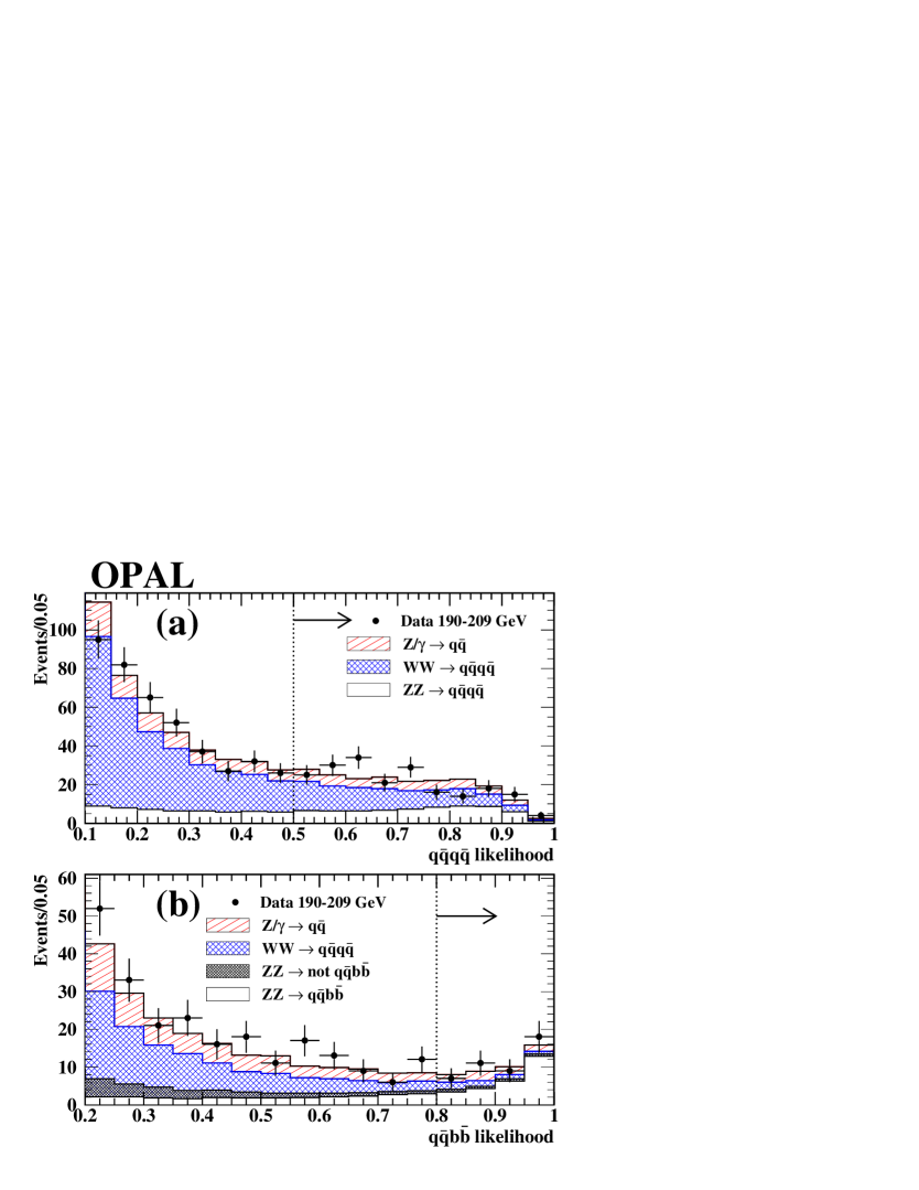
Figure 4: The combined distributions of likelihood discriminants used for all energies above 190 GeV. (a) $\mathrm{e^{+}}\mathrm{e^{-}}\to\mbox{$\mathrm{Z}$}\mbox{$\mathrm{Z}$}\to\mathrm{q}\overline{\mathrm{q}}\mathrm{q}\overline{\mathrm{q}}$ selection and (b) $\mathrm{e^{+}}\mathrm{e^{-}}\to\mbox{$\mathrm{Z}$}\mbox{$\mathrm{Z}$}\to\mathrm{q}\overline{\mathrm{q}}\mathrm{b}\overline{\mathrm{b}}$ selection. The dotted line and arrow show the position of the likelihood cut used to select ZZ events in each case.

$\sqrt{s}=190-209$ GeV

	Selection	$n_{\mathrm{obs}}$	$n_{\mathrm{SM}}$	$n_{\mathrm{ZZ}}$	$n_{\mathrm{back}}$	$\epsilon_{\mathrm{chan}}$	$B_{\mathrm{ZZ}}$	$L_{\mathrm{int}}$
								$(\mathrm{pb}^{-1})$
a	${\ell^{+}}{\ell^{-}}{\ell^{+}}{\ell^{-}}$	4	$3.55\pm 0.29$	$2.46\pm 0.09$	$1.08\pm 0.27$	$0.56\pm 0.02$	0.010	433.6
b	$\mathrm{e^{+}}\mathrm{e^{-}}\nu\overline{\nu}$	2	$3.71\pm 0.35$	$2.43\pm 0.31$	$1.28\pm 0.15$	$0.41\pm 0.05$	0.013	435.2
c	$\mu^{+}\mu^{-}\nu\overline{\nu}$	0	$4.30\pm 0.39$	$2.39\pm 0.33$	$1.91\pm 0.21$	$0.41\pm 0.06$	0.013	435.2
d	$\mathrm{q}\overline{\mathrm{q}}\mathrm{e^{+}}\mathrm{e^{-}}\,\&\,\overline{\mathrm{b}\overline{\mathrm{b}}\mathrm{e^{+}}\mathrm{e^{-}}}$	14	$11.6\pm 0.4$	$9.6\pm 0.3$	$1.98\pm 0.23$	$0.62\pm 0.03$	0.037	424.7
e	$\mathrm{q}\overline{\mathrm{q}}\mathrm{e^{+}}\mathrm{e^{-}}\,\&\,\mathrm{b}\overline{\mathrm{b}}\mathrm{e^{+}}\mathrm{e^{-}}$	3	$2.49\pm 0.19$	$2.20\pm 0.18$	$0.30\pm 0.07$	$0.51\pm 0.05$	0.010	424.7
f	$\mathrm{q}\overline{\mathrm{q}}\mu^{+}\mu^{-}\,\&\,\overline{\mathrm{b}\overline{\mathrm{b}}\mu^{+}\mu^{-}}$	15	$12.9\pm 0.4$	$12.1\pm 0.4$	$0.83\pm 0.12$	$0.77\pm 0.03$	0.037	424.7
g	$\mathrm{q}\overline{\mathrm{q}}\mu^{+}\mu^{-}\,\&\,\mathrm{b}\overline{\mathrm{b}}\mu^{+}\mu^{-}$	7	$2.59\pm 0.15$	$2.43\pm 0.14$	$0.16\pm 0.06$	$0.56\pm 0.05$	0.010	424.7
h	$\mathrm{q}\overline{\mathrm{q}}\tau^{+}\tau^{-}\,\&\,\overline{\mathrm{b}\overline{\mathrm{b}}\tau^{+}\tau^{-}}$	4	$5.35\pm 0.41$	$4.63\pm 0.39$	$0.72\pm 0.12$	$0.30\pm 0.03$	0.037	424.7
i	$\mathrm{q}\overline{\mathrm{q}}\tau^{+}\tau^{-}\,\&\,\mathrm{b}\overline{\mathrm{b}}\tau^{+}\tau^{-}$	0	$1.41\pm 0.19$	$1.19\pm 0.18$	$0.21\pm 0.06$	$0.28\pm 0.04$	0.010	424.7
j	$\mathrm{b}\overline{\mathrm{b}}\tau^{+}\tau^{-}\,\&\,\overline{\mathrm{q}\overline{\mathrm{q}}\tau^{+}\tau^{-}}$	1	$0.35\pm 0.10$	$0.29\pm 0.10$	$0.07\pm 0.03$	$0.07\pm 0.02$	0.010	424.7
k	$\mathrm{q}\overline{\mathrm{q}}\nu\overline{\nu}\,\&\,\overline{\mathrm{b}\overline{\mathrm{b}}\nu\overline{\nu}}$	51	$56.4\pm 2.8$	$30.3\pm 2.5$	$26.1\pm 1.2$	$0.33\pm 0.03$	0.219	422.1
l	$\mathrm{q}\overline{\mathrm{q}}\nu\overline{\nu}\,\&\,\mathrm{b}\overline{\mathrm{b}}\nu\overline{\nu}$	9	$8.45\pm 0.74$	$7.23\pm 0.71$	$1.22\pm 0.22$	$0.28\pm 0.03$	0.061	422.1
m	$\mathrm{q}\overline{\mathrm{q}}\mathrm{q}\overline{\mathrm{q}}\,\&\,\overline{\mathrm{q}\overline{\mathrm{q}}\mathrm{b}\overline{\mathrm{b}}}$	185	$180.5\pm 13.5$	$50.2\pm 3.1$	$130.3\pm 13.1$	$0.39\pm 0.03$	0.300	432.3
n	$\mathrm{q}\overline{\mathrm{q}}\mathrm{b}\overline{\mathrm{b}}\,\&\,\overline{\mathrm{q}\overline{\mathrm{q}}\mathrm{q}\overline{\mathrm{q}}}$	24	$21.9\pm 1.4$	$13.7\pm 0.8$	$8.14\pm 1.14$	$0.17\pm 0.01$	0.189	432.3
o	$\mathrm{q}\overline{\mathrm{q}}\mathrm{b}\overline{\mathrm{b}}\,\&\,\mathrm{q}\overline{\mathrm{q}}\mathrm{q}\overline{\mathrm{q}}$	21	$21.4\pm 1.2$	$16.1\pm 0.9$	$5.30\pm 0.74$	$0.20\pm 0.02$	0.189	432.3

Table 2: Observed number of events, $n_{\mathrm{obs}}$, the total Standard Model expectation, $n_{\mathrm{SM}}$, the expected number of $\mathrm{Z}$-pairs, $n_{\mathrm{ZZ}}$, background expectation, $n_{\mathrm{back}}$, and efficiencies, $\epsilon_{\mathrm{chan}}$, for the combined data sample. $B_{\mathrm{ZZ}}$ is the product branching ratio for the final state which is calculated directly from $\mathrm{Z}$ resonance data [6]. An overbar is used to indicate that events from a particular selection are rejected. Note that the efficiencies for selections with b-tags are given relative to the fraction of hadronic final states which contain a $\mathrm{Z}$ boson decaying to $\mathrm{b}\overline{\mathrm{b}}$. For selections of events with hadronic final states, but without b-tags, the efficiencies are relative to those expected hadronic final states which do not include a $\mathrm{Z}$ boson decaying to $\mathrm{b}\overline{\mathrm{b}}$. The errors on all quantities include contributions from the systematic uncertainties described in Section 3.6.

3.6 Systematic uncertainties

Systematic uncertainties have only a modest effect on our final result because of the large statistical error associated with the small number of $\mathrm{Z}$-pair events produced at LEP 2.

Detector systematic uncertainties for the $\mathrm{q}\overline{\mathrm{q}}{\ell^{+}}{\ell^{-}}$ and ${\ell^{+}}{\ell^{-}}{\ell^{+}}{\ell^{-}}$ selections without $\tau$-pairs in the final state are small because of the good separation of signal and background. In the $\mathrm{q}\overline{\mathrm{q}}{\ell^{+}}{\ell^{-}}$ channels possible mismodeling of the detector resolution is accounted for by smearing polar and azimuthal jet angles with a Gaussian width of 1^∘ and the energies by 5%. This gives systematic shifts smaller than 5%. These shifts are included in the systematic uncertainties on the efficiencies. In the $\mathrm{q}\overline{\mathrm{q}}\tau^{+}\tau^{-}$ selection, the additional systematic uncertainties in the efficiencies are determined by overlaying hadronic and tau decays taken from $\mathrm{Z}$ resonance data giving the dominant contribution to the total systematic uncertainty of 6.2%. In the ${\ell^{+}}{\ell^{-}}{\ell^{+}}{\ell^{-}}$ final state the largest effect (3%) is from the modeling of the multiplicity requirement which is important for final states containing $\tau$-pairs.

In the final states with neutrinos, ${\ell^{+}}{\ell^{-}}\nu\overline{\nu}$ and $\mathrm{q}\overline{\mathrm{q}}\nu\overline{\nu}$, tight cuts are needed to separate signal and background. In these selections detector effects can best be studied by comparing calibration data taken at the $\mathrm{Z}$ resonance with a simulation of the same process. In these cases, we add additional smearing to the total energy and momentum of the simulated events to match data and simulation on the $\mathrm{Z}$-resonance. We then apply the same smearing to the signal and background Monte Carlo simulations for the $\mathrm{Z}$-pair analyses. The reported efficiencies and backgrounds are accordingly corrected. The full difference is used as the systematic uncertainty in these cases. These differences give relative systematic uncertainties on the efficiency of 2.5% for the $\mathrm{e^{+}}\mathrm{e^{-}}\nu\overline{\nu}$ final state, 5.2% for the $\mu^{+}\mu^{-}\nu\overline{\nu}$ final state and 3.8% for $\mathrm{q}\overline{\mathrm{q}}\nu\overline{\nu}$ final state.

In the $\mathrm{q}\overline{\mathrm{q}}\mathrm{q}\overline{\mathrm{q}}$ inclusive analysis the sensitivity to the detector description of jet eneriges is much reduced by the use of kinematic fits. In this case the systematic uncertainties are determined by smearing the jet energies by an additional 5% and the jet directions by 1^∘ leading to a relative detector systematic uncertainty of 6%.

Another important detector effect comes from the simulation of the variables used by the OPAL b-tag which is discussed in Reference [10]. We allow for a common 5% uncertainty on the efficiency of the b-tag, consistent with our studies on $\mathrm{Z}$ resonance data and Monte Carlo simulation.

In each channel the signal and background Monte Carlo generators have been compared against alternative generators. In almost all cases the observed differences are consistent within the finite Monte Carlo statistics and the systematic uncertainty has been assigned accordingly.

The largest contribution to the systematic uncertainty from the model dependence of the background prediction is for the $\mathrm{q}\overline{\mathrm{q}}\mathrm{q}\overline{\mathrm{q}}$ and $\mathrm{q}\overline{\mathrm{q}}\mathrm{b}\overline{\mathrm{b}}$ final states. This uncertainty has been estimated by comparing the predictions of KORALW and grc4f for the $\mathrm{W}$-pair background, and the prediction of PYTHIA and KK2f for the background from hadronic 2-fermion production. The resulting uncertainty is 10% on the background for the inclusive selection and 20% for the background of the $\mathrm{q}\overline{\mathrm{q}}\mathrm{b}\overline{\mathrm{b}}$ selection [10]. The 10% uncertainty has been taken to be fully correlated between energy points and between the $\mathrm{q}\overline{\mathrm{q}}\mathrm{q}\overline{\mathrm{q}}$ and $\mathrm{q}\overline{\mathrm{q}}\mathrm{b}\overline{\mathrm{b}}$ selections. The correlated error on the $\mathrm{q}\overline{\mathrm{q}}\mathrm{b}\overline{\mathrm{b}}$ selection from uncertainties in the background due to b-tagging, has been absorbed into the overall b-tagging efficiency uncertainty.

In the ${\ell^{+}}{\ell^{-}}{\ell^{+}}{\ell^{-}}$ channel, which has a large background from two-photon events, we have compared the number of selected events at an early stage of the analysis with the Monte Carlo simulation and based our background systematic uncertainty on the level of agreement. This results in 20% systematic uncertainty on the background.

The efficiencies and backgrounds given for each energy point (see the Appendix and the summary Table 2) include the systematic uncertainties described in this section as well as errors from finite Monte Carlo statistics. Given the large statistical error from the small $\mathrm{Z}$-pair cross section we have employed the following conservative scheme to account for possible correlations among the systematic uncertainties:

1. The common correlated error from detector systematics, hadronization and kinematic distributions of the $\mathrm{Z}$-pair events is taken to be 3%. This is based primarily on the studies of the smearing of reconstructed jet and lepton directions.

2. The common systematic uncertainty for any channel including a b-tag is taken to be 5%.

3. As described above an uncertainty of 10% of the backgrounds is taken to be fully correlated among all $\mathrm{q}\overline{\mathrm{q}}\mathrm{q}\overline{\mathrm{q}}$ and $\mathrm{q}\overline{\mathrm{q}}\mathrm{b}\overline{\mathrm{b}}$ channels.

4. Based on generator level comparisons of kinematic distributions we conservatively assume a 2% correlated systematic uncertainty for the modeling of any changes to the physics description of the $\mathrm{Z}$ process when new physics is switched on. This is in addition to an overall uncertainty of 2% for the Standard Model total cross section prediction of the ZZTO calculation.

4 Cross section and branching ratios

At each center-of-mass energy point, information from all of the analyses is combined using a maximum likelihood fit to determine the production cross section for $\mathrm{e^{+}}\mathrm{e^{-}}\to\mbox{$\mathrm{Z}$}\mbox{$\mathrm{Z}$}$. The information which was used in the fits, as well as the Standard Model prediction for $\mathrm{Z}$-pair production, is summarized in Table 2. The details for each energy point are given in the Appendix. For each channel the tables give the number of events observed, $n_{\mathrm{obs}}$, the Standard Model prediction for all events, $n_{\mathrm{SM}}$, the expected signal, $n_{\mathrm{ZZ}}$, the expected background, $n_{\mathrm{back}}$, the efficiency $\epsilon_{\mathrm{chan}}$, and the integrated luminosity, $L_{\mathrm{int}}$. $B_{\mathrm{ZZ}}$ is the branching ratio of $\mathrm{Z}$-pairs to the given final state, calculated from $\mathrm{Z}$ resonance data [6]. In the table we give the overlap between the b-tag and non-b-tag analyses. Possible overlap between $\mathrm{q}\overline{\mathrm{q}}\mathrm{q}\overline{\mathrm{q}}$ and $\mathrm{q}\overline{\mathrm{q}}{\ell^{+}}{\ell^{-}}$ has been studied, and found to be an order of magnitude smaller than the overlap of $\mathrm{q}\overline{\mathrm{q}}\mathrm{q}\overline{\mathrm{q}}$ and $\mathrm{q}\overline{\mathrm{q}}\mathrm{b}\overline{\mathrm{b}}$ and has therefore been ignored.

Figure 5: The OPAL measurements of the NC2 $\mathrm{Z}$-pair production cross section. The middle of the shaded band shows the Standard Model prediction of the ZZTO calculation. The band indicates a theoretical uncertainty of $\pm 2$%. The error bars on the data show the combined statistical and systematic uncertainty, the horizontal marks indicate the extent of the statistical errors. Data from $\sqrt{s}$ near 183 GeV and 189 GeV are from Reference [3].

Figure 6: The OPAL measurements of the NC2 $\mathrm{Z}$-pair differential cross section $\mathrm{d}\sigma_{\mathrm{ZZ}}/\mathrm{d}|\cos\theta_{\mathrm{Z}}|$. The curves show the prediction of the YFSZZ Monte Carlo for the differential cross section, which has been normalized to agree with the total cross section of the ZZTO calculation. The error bars show the combined statistical and systematic uncertainty. The arrow shows the 95% confidence level upper limit for the one case where the minimum of the negative log likelihood function was at zero.

The cross section at each energy is determined with a maximum likelihood fit using Poisson probability densities convolved with Gaussians to describe the uncertainties on efficiencies and backgrounds. The expected number of events in each channel, $\mu_{\mathrm{e}}$, as function of the $\mathrm{Z}$-pair cross section, $\sigma_{\mathrm{ZZ}}$, is given by

$$\mu_{\mathrm{e}}=\sigma_{\mathrm{ZZ}}L_{\mathrm{int}}\epsilon_{\mathrm{chan}}B_{\mathrm{ZZ}}+n_{\mathrm{back}}.$$ (3)

The efficiencies, $\epsilon_{\mathrm{chan}}$, include the effects of off-shell $\mathrm{Z}$ bosons that are produced outside of our kinematic acceptance. The correlated systematic uncertainties described in the last section are implemented by introducing additional parameters which are constrained with Gaussian probability densities given by the size of the systematic uncertainty. Our main results, the NC2 $\mathrm{Z}$-pair cross sections obtained from the fits, are

$$\begin{array}[]{lcll}\sigma_{\mathrm{ZZ}}(192\ \mathrm{GeV})&=&1.29\ ^{+0.47}_{-0.40}\ {}^{+0.12}_{-0.09}&\mathrm{pb}\\ &&&\\ \sigma_{\mathrm{ZZ}}(196\ \mathrm{GeV})&=&1.13\ ^{+0.26}_{-0.24}\ {}^{+0.08}_{-0.07}&\mathrm{pb}\\ &&&\\ \sigma_{\mathrm{ZZ}}(200\ \mathrm{GeV})&=&1.05\ ^{+0.25}_{-0.22}\ {}^{+0.07}_{-0.06}&\mathrm{pb}\\ &&&\\ \sigma_{\mathrm{ZZ}}(202\ \mathrm{GeV})&=&0.79\ ^{+0.35}_{-0.29}\ {}^{+0.08}_{-0.05}&\mathrm{pb}\\ &&&\\ \sigma_{\mathrm{ZZ}}(205\ \mathrm{GeV})&=&1.07\ ^{+0.27}_{-0.24}\ {}^{+0.08}_{-0.07}&\mathrm{pb}\\ &&&\\ \sigma_{\mathrm{ZZ}}(207\ \mathrm{GeV})&=&0.97\ ^{+0.19}_{-0.18}\ {}^{+0.06}_{-0.05}&\mathrm{pb}.\\ \end{array}$$

The first error is statistical and the second error is systematic. The systematic errors are obtained from the quadrature difference of the errors when running the fit with and without systematic uncertainties. The comparison of these measurements with the ZZTO prediction is shown in Figure 5. The results are consistent with the Standard Model prediction.

We have also analyzed our data in four bins of $|\cos\theta_{\mathrm{Z}}|$ where $\theta_{Z}$ is the polar angle of the $\mathrm{Z}$ bosons. Except for channels with one $\mathrm{Z}$ boson decaying to neutrinos, the value of $|\cos\theta_{\mathrm{Z}}|$ is determined from kinematic fits which assume no initial-state radiation. In the ${\ell^{+}}{\ell^{-}}\nu\overline{\nu}$ and $\mathrm{q}\overline{\mathrm{q}}\nu\overline{\nu}$ channels, the direction is determined from the reconstructed direction of the visible $\mathrm{Z}$. The comparison of the expected and observed differential cross sections is shown in Figure 6. The data in Figure 6 have been corrected for small amounts of bin migration assuming the Standard Model prediction.

In order to check the consistency of our result with the Standard Model, we have performed a maximum likelihood fit in which the Standard Model ZZTO prediction is scaled by an overall factor $R$. The fit is based on individual measurements for each channel given in the Appendix in Tables 5 to 10 as well as the data presented in Reference [3]. The treatment of the correlated systematic uncertainties is outlined in Section 3.6. The fit yields

$$R=1.06^{+0.11}_{-0.10}$$

where the error includes the correlated experimental systematic uncertainty (3%) and the theoretical uncertainty on the ZZTO prediction (2%). In a separate fit, we allowed the branching ratio of $\mathrm{Z}$ bosons to b quarks, BR$(\mbox{$\mathrm{Z}$}\to\mathrm{b}\overline{\mathrm{b}})$, to be a free parameter in the fits at each of the energy points. The results are shown in Figure 7. The BR$(\mbox{$\mathrm{Z}$}\to\mathrm{b}\overline{\mathrm{b}})$ values tend to lie above the measured value from LEP 1 data; combining all energies, the average value is 0.196$\pm$0.032, which is 1.3 standard deviations above the LEP 1 measurement of 0.1514$\pm$0.0005[6].

Figure 7: Determination of Br$(\mbox{$\mathrm{Z}$}\to\mathrm{b}\overline{\mathrm{b}})$ from $\mathrm{Z}$$\mathrm{Z}$ events. The line shows the measured value from LEP 1 data. Only statistical errors are shown. The data have a common systematic uncertainty which amounts to approximately 5% of the expected branching ratio. The 189 GeV point is from Reference [3]; at 183 GeV the $\mathrm{Z}$$\mathrm{Z}$ event samples were too small to allow a meaningful measurement to be obtained.

5 Limits on anomalous triple gauge couplings

Limits on anomalous triple gauge couplings were set using the measured cross sections and kinematic information from an optimal observable (OO) method for the $\mathrm{q}\overline{\mathrm{q}}\mathrm{q}\overline{\mathrm{q}}$, $\mathrm{q}\overline{\mathrm{q}}\mathrm{b}\overline{\mathrm{b}}$ and $\mathrm{q}\overline{\mathrm{q}}{\ell^{+}}{\ell^{-}}$ selections. In this study we vary the real part of the $\mathrm{Z}$$\mathrm{Z}$$\mathrm{Z}$ and $\mbox{$\mathrm{Z}$}\mbox{$\mathrm{Z}$}\gamma$ anomalous couplings parameterized by $f_{4}^{\mathrm{ZZZ}}$, $f_{5}^{\mathrm{ZZZ}}$, $f_{4}^{\mathrm{ZZ\gamma}}$ and $f_{5}^{\mathrm{ZZ\gamma}}$ as defined in Reference [7] and implemented in the YFSZZ Monte Carlo. In most cases, the real parts of each coupling were varied separately with all others fixed to zero.

The OO analysis used here is described in detail in Reference [41]. Since the effective Lagrangian used to describe the anomalous couplings is linear in the couplings, the resulting differential cross section is parabolic and can be parameterized, for a single non-zero coupling $\alpha_{i}$, as

$$\frac{\mathrm{d}\sigma}{\mathrm{d}\Omega}=S^{(0)}(\Omega)+\alpha_{i}S^{(1)}_{i}(\Omega)+\alpha_{i}^{2}S^{(2)}_{i}(\Omega)$$ (4)

where $\Omega$ is the phase-space point based on the four-momenta of the four out-going fermions from the $\mathrm{Z}$ decays. The optimal observables are defined as

$$\begin{array}[]{lcl}{\cal O}_{1}^{i}&\equiv&S^{(1)}_{i}(\Omega)/S^{(0)}(\Omega)\\ {\cal O}_{2}^{i}&\equiv&S^{(2)}_{i}(\Omega)/S^{(0)}(\Omega).\\ \end{array}$$ (5)

To reduce the dependence of our analysis on the tails of the ${\cal O}_{1}^{i}$ and ${\cal O}_{2}^{i}$ distribution, extreme values of ${\cal O}_{1}^{i}$ and ${\cal O}_{2}^{i}$ were rejected when calculating the mean values. These cuts were chosen based on the expected distribution of ${\cal O}_{1}^{i}$ and ${\cal O}_{2}^{i}$ calculated from Monte Carlo and typically reject a few percent of the expected events.

The expected average values of the first order optimal observable, $\langle{\cal O}_{1}\rangle$, and the second order optimal observable, $\langle{\cal O}_{2}\rangle$, were calculated using the YFSZZ matrix element to reweight accepted events from the signal Monte Carlo. The same cuts on extreme values of ${\cal O}_{1}^{i}$ and ${\cal O}_{2}^{i}$ were used in data and Monte Carlo simulation. The parameterization used was of the form

$$\begin{array}[]{lcl}\langle{\cal O}_{1}\rangle&=&\frac{\mbox{$p_{0}+p_{1}\alpha+p_{2}\alpha^{2}$}}{\mbox{$d_{0}+d_{1}\alpha+d_{2}\alpha^{2}$}}\\ &&\\ \langle{\cal O}_{2}\rangle&=&\frac{\mbox{$q_{0}+q_{1}\alpha+q_{2}\alpha^{2}$}}{\mbox{$d_{0}+d_{1}\alpha+d_{2}\alpha^{2}$}}\\ \end{array}$$ (6)

where $\alpha$ is the value of the anomalous coupling and the coefficients are determined separately for each selection, energy and type of anomalous coupling. Note that the mean values of the optimal observables are normalized to the observed number of events and do not depend on the cross section which is considered separately below. This can be seen in Equation (6) by noting that the polynomial $d_{0}+d_{1}\alpha+d_{2}\alpha^{2}$ parameterizes the change in cross section with anomalous coupling. The average value of the optimal observable for the exclusive $\mathrm{q}\overline{\mathrm{q}}\mathrm{e^{+}}\mathrm{e^{-}}$, $\mathrm{q}\overline{\mathrm{q}}\mu^{+}\mu^{-}$ and three categories of $\mathrm{q}\overline{\mathrm{q}}\mathrm{q}\overline{\mathrm{q}}$ events ( $\mathrm{q}\overline{\mathrm{q}}\mathrm{q}\overline{\mathrm{q}}\,\&\,\overline{\mathrm{q}\overline{\mathrm{q}}\mathrm{b}\overline{\mathrm{b}}}$, $\mathrm{q}\overline{\mathrm{q}}\mathrm{b}\overline{\mathrm{b}}\,\&\,\mathrm{q}\overline{\mathrm{q}}\mathrm{q}\overline{\mathrm{q}}$ and $\mathrm{q}\overline{\mathrm{q}}\mathrm{b}\overline{\mathrm{b}}\,\&\,\overline{\mathrm{q}\overline{\mathrm{q}}\mathrm{q}\overline{\mathrm{q}}}$ ) were calculated from the data at each energy between 190 GeV and 207 GeV. The statistical uncertainties on these values were parameterized with a covariance matrix determined from high statistics Standard Model signal and background Monte Carlo simulations. The covariance matrix was then scaled to match the number of events observed in the data.

The systematic uncertainties were taken into account by varying the modeling of the Standard Model signal and the backgrounds. Any deviations were interpreted as a systematic error and included in the covariance matrix. The error associated with the physics simulation of the signal was determined by comparing the values of $\langle{\cal O}_{1}\rangle$ and $\langle{\cal O}_{2}\rangle$ determined from reweighting the YFSZZ and grc4f Monte Carlo event samples. The error in the background determination was evaluated by using the alternative background simulations described in Section 3.6. These differences were taken to be fully correlated among energies for a given final state. The systematic uncertainties associated with the accuracy of the event reconstruction were evaluated by applying additional smearing to the energies and angles of the reconstructed jets and leptons. The resulting contributions to the covariance matrix were taken to be fully correlated among all five final state selections. The resulting $\chi^{2}$ functions, converted to likelihood curves, are shown as dashed lines in Figure 8.

For those channels used in the OO analysis, we use in addition only the cross section integrated over $|\cos\theta_{\mathrm{Z}}|$. For channels that are not used in the OO analysis, the cross section in four bins of $|\cos\theta_{\mathrm{Z}}|$ is used. The ZZTO calculation is used for the prediction of the Standard Model integrated cross section. The change in the $\mathrm{Z}$-pair cross section as a function of $|\cos\theta_{\mathrm{Z}}|$ and the values of the anomalous couplings is parameterized using the YFSZZ Monte Carlo. In addition, the selection efficiencies for all final states are parameterized as a function of the couplings and for each bin in $|\cos\theta_{\mathrm{Z}}|$. An uncertainty of 10%, dominated by Monte Carlo statistical errors, is assigned to the correction we applied to all of these efficiencies. The resulting likelihood curves based on cross-section measurements are shown as dotted lines in Figure 8. These cross-section results include data at 183 GeV and 189 GeV from Reference [3].

Combining the likelihood associated with the $\chi^{2}$ fit and the likelihood curve from the cross-section fit, the 95% confidence level (C.L.) limits on the anomalous couplings were obtained and are given in Table 3. The combined likelihood curves are shown as solid lines in Figure 8.

Equation (4) can easily be extended to the case of two non-zero couplings and the constraints can be derived for pairs of couplings [41]. Note that for the two-dimensional OO fits, the event sample is slightly different from that used in the one-dimensional OO fits, as cuts are placed on the values of optimal observables for more than one coupling. The constraint from the expected cross sections can also be calculated for two non-zero couplings. The resulting 95% confidence level contours in the $f_{4}$ and $f_{5}$ plane, including both OO and cross-section constraints, are shown in Figure 9. The 95% confidence level corresponds to a change in log likelihood of 3.0 from the minimum value.

Figure 8: The negative log likelihood as a function of the real part of the four anomalous couplings: dotted, constraint from cross-section information; dashed, constraint from optimal observables analysis; and solid, sum. The 95% confidence level corresponds to a change in log likelihood of 1.92 from the minimum value. These results are dominated by the $190-209$ GeV data, but also include the OPAL data from 183 GeV and 189 GeV presented in Reference [3].

Figure 9: The 95% confidence level contours, corresponding to a change of 3.0 in the log likelihood from the minimum, for (a) the $f_{4}^{\mathrm{ZZ\gamma}}-f_{4}^{\mathrm{ZZZ}}$ plane and (b) the $f_{5}^{\mathrm{ZZ\gamma}}-f_{5}^{\mathrm{ZZZ}}$ plane. These results include all channels and all energies, including OPAL data from 183 GeV and 189 GeV presented in Reference [3]. The star shows the location of the minimum, the solid dot the Standard Model.

Coupling	95% C.L. lower limit	95% C.L. upper limit
$f_{4}^{\mathrm{ZZZ}}$	$-0.45$	$0.58$
$f_{5}^{\mathrm{ZZZ}}$	$-0.94$	$0.25$
$f_{4}^{\mathrm{ZZ\gamma}}$	$-0.32$	$0.33$
$f_{5}^{\mathrm{ZZ\gamma}}$	$-0.71$	$0.59$

Table 3: The 95% confidence level limits on possible anomalous triple gauge couplings. These results include all channels and all energies, including the OPAL data from 183 GeV and 189 GeV presented in Reference [3].

6 Limits on low scale gravity theories with large extra dimensions

We have also examined the possible effects of low scale gravity (LSG) theories with large extra dimensions [42] on the $\mathrm{Z}$-pair cross section. In the LSG theories considered here, gravity is allowed to propagate in $D=4+n$ dimensions, while all other particles are confined to four dimensional space. Newtonian gravity in three spatial dimensions holds if

$$M^{2}_{\mathrm{Planck}}\propto R^{n}M_{D}^{(n+2)}$$ (7)

where $M_{\mathrm{Planck}}$ is the Planck scale in the usual four dimensions, $M_{D}$ is the Planck scale in the D-dimensional space, and $R$ is the compactification radius of the $n$ extra dimensions. The case of $n=1$ is excluded by cosmological observations. For the case of $n=2$, severe constraints are imposed by studies of the gravitational interaction on sub-millimeter distance scales[43, 44].

Because gravity can propagate in the extra dimensions, the amplitude for $\mathrm{Z}$-pair production has leading order contributions from the $s$-channel exchange of Kaluza-Klein graviton states. The effective theory at LEP 2 energies is sensitive to the mass scale $M_{s}$ that is used to regulate ultraviolet divergences. $M_{s}$ is expected to be of the same order of magnitude as $M_{D}$. Using this mass scale, $M_{s}$, a contribution to the Born level amplitude that is proportional to $\lambda/M_{s}^{4}$ is obtained. Here $\lambda$ is an effective coupling. In this paper we use the definition of $M_{s}$ given in Reference [45] for our main result.

In order to search for deviations from the Standard Model compatible with LSG theories, the differential $\mathrm{Z}$-pair cross section is written as

$$\frac{\mathrm{d}\sigma_{\mathrm{ZZ}}}{\mathrm{d}\cos\theta_{\mathrm{Z}}}=\\ \frac{\alpha\beta}{\pi s}\sum_{\kappa,\epsilon_{+},\epsilon_{-}}C^{2}_{\Gamma_{\mathrm{Z}}}(s,\cos\theta)\left|{C}^{\mathrm{SM}}_{\mathrm{ISR}}(s){\cal M}^{\mathrm{SM}}_{\mathrm{born}}(\kappa,\epsilon_{+},\epsilon_{-},s,t)+{C}^{\mathrm{grav}}_{\mathrm{ISR}}(s){\cal M}_{\mathrm{gravity}}(\kappa,\epsilon_{+},\epsilon_{-},s,t)\right|^{2}$$ (8)

where $\alpha$ is the fine structure constant, $s$ and $t$ are the Mandelstam variables, $\kappa$ is the electron helicity, $\epsilon_{+}$ and $\epsilon_{-}$ are the polarizations of the $\mathrm{Z}$ boson, $\beta$ is the $\mathrm{Z}$ velocity, and ${\cal M}^{\mathrm{SM}}_{\mathrm{born}}(\kappa,\epsilon_{+},\epsilon_{-},s,t)$ and ${\cal M}_{\mathrm{gravity}}(\kappa,\epsilon_{+},\epsilon_{-},s,t)$ are the Born level SM and gravity matrix elements [9]. Here ${\cal M}_{\mathrm{gravity}}(\kappa,\epsilon_{+},\epsilon_{-},s,t)$ is proportional to $\frac{\lambda}{M_{s}^{4}}$. The factor $C_{\Gamma_{\mathrm{Z}}}(s,\cos\theta)$ corrects for the effects of the finite width of the $\mathrm{Z}$. The factors $C^{\mathrm{SM}}_{\mathrm{ISR}}(s)$ and $C^{\mathrm{grav}}_{\mathrm{ISR}}(s)$ correct for initial-state radiation.

The factors $C^{\mathrm{SM}}_{\mathrm{ISR}}$(s), and $C^{\mathrm{grav}}_{\mathrm{ISR}}(s)$ are given by

$$C=\sqrt{\frac{\sigma^{\mathrm{YFSZZ}}_{\mathrm{ISR}}}{\sigma^{\mathrm{YFSZZ}}_{\mathrm{Born}}}}$$ (9)

where $\sigma^{\mathrm{YFSZZ}}_{\mathrm{ISR}}$ is the YFSZZ cross section with ISR and $\sigma^{\mathrm{YFSZZ}}_{\mathrm{Born}}$ is the Born level YFSZZ cross section. The ISR correction for Standard Model $\mathrm{Z}$ production, $C^{\mathrm{SM}}_{\mathrm{ISR}}$(s), is estimated by running YFSZZ with all anomalous couplings off. For the case of gravity, $C^{\mathrm{grav}}_{\mathrm{ISR}}(s)$ is estimated by using a choice of anomalous couplings which causes the s-channel to dominate. These factors range from 0.84 at 183 GeV to 0.93 at 207 GeV. $C^{\mathrm{SM}}_{\mathrm{ISR}}(s)$ and $C^{\mathrm{grav}}_{\mathrm{ISR}}(s)$ differ from each other by no more than 5%.

The effect of the finite $\mathrm{Z}$ width depends on $|\cos\theta_{\mathrm{Z}}|$ and is obtained from

$$C_{\Gamma_{\mathrm{Z}}}(s,\cos\theta)=\sqrt{\frac{\sigma^{\mathrm{YFSZZ}}_{|\cos\theta_{\mathrm{Z}}|}}{\sigma^{\mathrm{\Gamma_{Z}=0}}_{|\cos\theta_{\mathrm{Z}}|}}}$$ (10)

where $\sigma^{\mathrm{\Gamma_{Z}=0}}$ is the prediction of Equation (8) with $C_{\Gamma_{\mathrm{Z}}}(s,\cos\theta)=1$ and $\lambda=0$. At center-of-mass energies above 195 GeV, $C_{\Gamma_{\mathrm{Z}}}(s,\cos\theta)$ is within 5% of unity.

In our fit, Equation (8) is used only to compute the expected difference in cross section between the Standard Model with and without LSG switched on. As in the case of the anomalous couplings, the prediction of ZZTO for the Standard Model cross section is used and the expected angular dependence is taken from YFSZZ.

A maximum likelihood fit is performed in four bins of $|\cos\theta|$ for each selection and energy point. We also use previously published [3] data binned in four bins of $|\cos\theta|$ from 189 GeV and the integrated cross section from 183 GeV. The fit yields

$$\lambda/M_{s}^{4}=2.6\pm 2.3\ \mathrm{TeV}^{-4}.$$

The likelihood function is shown in Figure 10 and is approximately parabolic. Note that with the sign convention of Reference [45] positive values of $\lambda/M_{s}^{4}$ give a positive contribution to the cross section. Because our measured values of the cross sections are on average slightly larger than the Standard Model prediction (see Figure 6 and the value for $R$ given in Section 4), the central value for $\lambda/M_{s}^{4}$ is also positive.

If we assume that the a priori probability for a theory to be true is uniform in the variable $\lambda/M_{s}^{4}$ we can obtain limits on $M_{s}$ for a variety of theoretical approaches using the likelihood curve for $\lambda/M_{s}^{4}$. First, using the notation of Reference [45], we consider separately theories with $\lambda=+1$, which correspond to positive values of $\lambda/M^{4}_{s}$, and with $\lambda=-1$ which correspond to negative values of $\lambda/M^{4}_{s}$. In the first (second) case our prior assumes all values of $\lambda/M^{4}_{s}>0.0$ ( $\lambda/M^{4}_{s}<0.0$) are equally likely. We also use the approximation that the log-likelihood curve is parabolic. The resulting limits on $M_{s}$ are given in Table 4.

In the approach of Reference [46] a summation of higher order terms is used which eliminates the dependence of the prediction on $\lambda$. Comparing References [45] and [46] limits on $M_{s}$ can be determined, as a function of the number of large extra dimensions, $n$, using the substitution

$$\frac{\lambda}{M_{s}^{4}}\Rightarrow-\pi\frac{s^{\frac{n}{2}-1}}{M_{s}^{n+2}}I_{n}\left(\frac{M_{s}}{\sqrt{s}}\right)$$ (11)

where the integrals $I_{n}(\frac{M_{s}}{\sqrt{s}})$ are given in Equation B.8 of Reference [46]. As the integrals $I_{n}$ are negative for all values of $n$, limits on $M_{s}$ correspond to the $\lambda=+1$ case shown in Figure 10. These limits on $M_{s}$ as a function of $n$ are given in Table 4.

Parameter	95% C.L. lower limit on $M_{s}$
Coupling	Method of Reference [45]
$\lambda=+1$	0.62 TeV
$\lambda=-1$	0.76 TeV
Number of extra dimensions	Method of Reference [46]
$n=2$	0.92 TeV
$n=3$	0.82 TeV
$n=4$	0.73 TeV
$n=5$	0.67 TeV
$n=6$	0.62 TeV
$n=7$	0.59 TeV

Table 4: The 95% confidence level on $M_{s}$ using the approach of References [45] and [46]. These results include all channels and all energies, including the OPAL data from 183 GeV and 189 GeV presented in Reference [3].

Figure 10: The negative log likelihood as a function of the $\lambda/M^{4}_{s}$. Limits on $M_{s}$ are determined separately for theories with $\lambda=+1$, which correspond to positive values of $\lambda/M^{4}_{s}$ and $\lambda=-1$ which correspond to negative values of $\lambda/M^{4}_{s}$. The dashed lines indicate the allowed 95% confidence level regions obtained in the two cases. These results are dominated by the $190-209$ GeV data, but also include the OPAL data from 183 GeV and 189 GeV presented in Reference [3].

7 Conclusion

The process $\mathrm{e^{+}}\mathrm{e^{-}}\to\mbox{$\mathrm{Z}$}\mbox{$\mathrm{Z}$}$ has been studied at center-of-mass energies between 190 GeV and 209 GeV using the final states ${\ell^{+}}{\ell^{-}}{\ell^{+}}{\ell^{-}}$, ${\ell^{+}}{\ell^{-}}\nu\overline{\nu}$, $\mathrm{q}\overline{\mathrm{q}}{\ell^{+}}{\ell^{-}}$, $\mathrm{q}\overline{\mathrm{q}}\nu\overline{\nu}$, and $\mathrm{q}\overline{\mathrm{q}}\mathrm{q}\overline{\mathrm{q}}$. The number of observed events, the background expectation from Monte Carlo and the calculated efficiencies have been combined to measure the NC2 cross section for the process $\mathrm{e^{+}}\mathrm{e^{-}}\to\mbox{$\mathrm{Z}$}\mbox{$\mathrm{Z}$}$. The measured cross sections for the six energy points are:

$$\begin{array}[]{lcll}\sigma_{\mathrm{ZZ}}(192\ \mathrm{GeV})&=&1.29\ ^{+0.47}_{-0.40}\ {}^{+0.12}_{-0.09}&\mathrm{pb}\\ &&&\\ \sigma_{\mathrm{ZZ}}(196\ \mathrm{GeV})&=&1.13\ ^{+0.26}_{-0.24}\ {}^{+0.08}_{-0.07}&\mathrm{pb}\\ &&&\\ \sigma_{\mathrm{ZZ}}(200\ \mathrm{GeV})&=&1.05\ ^{+0.25}_{-0.22}\ {}^{+0.07}_{-0.06}&\mathrm{pb}\\ &&&\\ \sigma_{\mathrm{ZZ}}(202\ \mathrm{GeV})&=&0.79\ ^{+0.35}_{-0.29}\ {}^{+0.08}_{-0.05}&\mathrm{pb}\\ &&&\\ \sigma_{\mathrm{ZZ}}(205\ \mathrm{GeV})&=&1.07\ ^{+0.27}_{-0.24}\ {}^{+0.08}_{-0.07}&\mathrm{pb}\\ &&&\\ \sigma_{\mathrm{ZZ}}(207\ \mathrm{GeV})&=&0.97\ ^{+0.19}_{-0.18}\ {}^{+0.06}_{-0.05}&\mathrm{pb}.\\ \end{array}$$

The measurements at all energies are consistent with the Standard Model expectations. Using information from the cross-section measurements and from the optimal observables, no evidence is found for anomalous neutral-current triple gauge couplings. The 95% confidence level limits are listed in Table 3. We have also derived limits on low scale gravity theories with large extra dimensions which are summarized in Table 4.

Appendix   Selected events at individual energies

The information which was used in the cross-section fit is summarized in Tables 5 to 10. For each channel, the tables give the number of events observed, $n_{\mathrm{obs}}$, the Standard Model prediction for all events, $n_{\mathrm{SM}}$, the expected signal, $n_{\mathrm{ZZ}}$, the expected background, $n_{\mathrm{back}}$, the efficiency $\epsilon_{\mathrm{chan}}$, and the integrated luminosity, $L_{\mathrm{int}}$. Note that $n_{\mathrm{SM}}$ as it appears in the tables is not always exactly $n_{\mathrm{back}}+n_{\mathrm{ZZ}}$ due to rounding.

$\sqrt{s}=192$ GeV

	Selection	$n_{\mathrm{obs}}$	$n_{\mathrm{SM}}$	$n_{\mathrm{ZZ}}$	$n_{\mathrm{back}}$	$\epsilon_{\mathrm{chan}}$	$B_{\mathrm{ZZ}}$	$L_{\mathrm{int}}$
								$(\mathrm{pb}^{-1})$
a	${\ell^{+}}{\ell^{-}}{\ell^{+}}{\ell^{-}}$	0	$0.28\pm 0.05$	$0.13\pm 0.01$	$0.14\pm 0.05$	$0.57\pm 0.02$	0.010	29.1
b	$\mathrm{e^{+}}\mathrm{e^{-}}\nu\overline{\nu}$	0	$0.21\pm 0.03$	$0.12\pm 0.02$	$0.09\pm 0.03$	$0.38\pm 0.05$	0.013	29.1
c	$\mu^{+}\mu^{-}\nu\overline{\nu}$	0	$0.24\pm 0.04$	$0.13\pm 0.02$	$0.11\pm 0.03$	$0.43\pm 0.06$	0.013	29.1
d	$\mathrm{q}\overline{\mathrm{q}}\mathrm{e^{+}}\mathrm{e^{-}}\,\&\,\overline{\mathrm{b}\overline{\mathrm{b}}\mathrm{e^{+}}\mathrm{e^{-}}}$	0	$0.65\pm 0.04$	$0.53\pm 0.02$	$0.12\pm 0.03$	$0.64\pm 0.03$	0.037	28.6
e	$\mathrm{q}\overline{\mathrm{q}}\mathrm{e^{+}}\mathrm{e^{-}}\,\&\,\mathrm{b}\overline{\mathrm{b}}\mathrm{e^{+}}\mathrm{e^{-}}$	1	$0.13\pm 0.01$	$0.11\pm 0.01$	$0.02\pm 0.01$	$0.47\pm 0.05$	0.010	28.6
f	$\mathrm{q}\overline{\mathrm{q}}\mu^{+}\mu^{-}\,\&\,\overline{\mathrm{b}\overline{\mathrm{b}}\mu^{+}\mu^{-}}$	2	$0.73\pm 0.04$	$0.65\pm 0.02$	$0.08\pm 0.03$	$0.79\pm 0.03$	0.037	28.6
g	$\mathrm{q}\overline{\mathrm{q}}\mu^{+}\mu^{-}\,\&\,\mathrm{b}\overline{\mathrm{b}}\mu^{+}\mu^{-}$	0	$0.15\pm 0.01$	$0.13\pm 0.01$	$0.01\pm 0.01$	$0.59\pm 0.05$	0.010	28.6
h	$\mathrm{q}\overline{\mathrm{q}}\tau^{+}\tau^{-}\,\&\,\overline{\mathrm{b}\overline{\mathrm{b}}\tau^{+}\tau^{-}}$	0	$0.28\pm 0.03$	$0.25\pm 0.02$	$0.02\pm 0.01$	$0.31\pm 0.03$	0.037	28.6
i	$\mathrm{q}\overline{\mathrm{q}}\tau^{+}\tau^{-}\,\&\,\mathrm{b}\overline{\mathrm{b}}\tau^{+}\tau^{-}$	0	$0.07\pm 0.01$	$0.05\pm 0.01$	$0.02\pm 0.01$	$0.23\pm 0.04$	0.010	28.6
j	$\mathrm{b}\overline{\mathrm{b}}\tau^{+}\tau^{-}\,\&\,\overline{\mathrm{q}\overline{\mathrm{q}}\tau^{+}\tau^{-}}$	0	$0.03\pm 0.01$	$0.02\pm 0.01$	$0.01\pm 0.01$	$0.10\pm 0.03$	0.010	28.6
k	$\mathrm{q}\overline{\mathrm{q}}\nu\overline{\nu}\,\&\,\overline{\mathrm{b}\overline{\mathrm{b}}\nu\overline{\nu}}$	3	$3.06\pm 0.22$	$1.67\pm 0.14$	$1.40\pm 0.17$	$0.34\pm 0.03$	0.219	28.6
l	$\mathrm{q}\overline{\mathrm{q}}\nu\overline{\nu}\,\&\,\mathrm{b}\overline{\mathrm{b}}\nu\overline{\nu}$	1	$0.43\pm 0.05$	$0.36\pm 0.03$	$0.07\pm 0.03$	$0.27\pm 0.03$	0.061	28.6
m	$\mathrm{q}\overline{\mathrm{q}}\mathrm{q}\overline{\mathrm{q}}\,\&\,\overline{\mathrm{q}\overline{\mathrm{q}}\mathrm{b}\overline{\mathrm{b}}}$	27	$17.6\pm 1.4$	$3.8\pm 0.3$	$13.8\pm 1.4$	$0.56\pm 0.04$	0.300	29.1
n	$\mathrm{q}\overline{\mathrm{q}}\mathrm{b}\overline{\mathrm{b}}\,\&\,\overline{\mathrm{q}\overline{\mathrm{q}}\mathrm{q}\overline{\mathrm{q}}}$	2	$0.93\pm 0.11$	$0.52\pm 0.04$	$0.42\pm 0.10$	$0.12\pm 0.01$	0.189	29.1
o	$\mathrm{q}\overline{\mathrm{q}}\mathrm{b}\overline{\mathrm{b}}\,\&\,\mathrm{q}\overline{\mathrm{q}}\mathrm{q}\overline{\mathrm{q}}$	1	$1.68\pm 0.13$	$1.21\pm 0.07$	$0.47\pm 0.11$	$0.28\pm 0.02$	0.189	29.1

Table 5: The 192 GeV data. The description of the entries is given in the caption of Table 2.

$\sqrt{s}=196$ GeV

	Selection	$n_{\mathrm{obs}}$	$n_{\mathrm{SM}}$	$n_{\mathrm{ZZ}}$	$n_{\mathrm{back}}$	$\epsilon_{\mathrm{chan}}$	$B_{\mathrm{ZZ}}$	$L_{\mathrm{int}}$
								$(\mathrm{pb}^{-1})$
a	${\ell^{+}}{\ell^{-}}{\ell^{+}}{\ell^{-}}$	1	$0.58\pm 0.10$	$0.37\pm 0.01$	$0.21\pm 0.10$	$0.56\pm 0.02$	0.010	72.5
b	$\mathrm{e^{+}}\mathrm{e^{-}}\nu\overline{\nu}$	1	$0.66\pm 0.08$	$0.37\pm 0.05$	$0.28\pm 0.06$	$0.42\pm 0.06$	0.013	72.7
c	$\mu^{+}\mu^{-}\nu\overline{\nu}$	0	$0.72\pm 0.10$	$0.37\pm 0.05$	$0.36\pm 0.08$	$0.41\pm 0.06$	0.013	72.7
d	$\mathrm{q}\overline{\mathrm{q}}\mathrm{e^{+}}\mathrm{e^{-}}\,\&\,\overline{\mathrm{b}\overline{\mathrm{b}}\mathrm{e^{+}}\mathrm{e^{-}}}$	2	$2.05\pm 0.16$	$1.58\pm 0.07$	$0.47\pm 0.14$	$0.67\pm 0.03$	0.037	71.3
e	$\mathrm{q}\overline{\mathrm{q}}\mathrm{e^{+}}\mathrm{e^{-}}\,\&\,\mathrm{b}\overline{\mathrm{b}}\mathrm{e^{+}}\mathrm{e^{-}}$	0	$0.39\pm 0.04$	$0.34\pm 0.03$	$0.05\pm 0.02$	$0.52\pm 0.05$	0.010	71.3
f	$\mathrm{q}\overline{\mathrm{q}}\mu^{+}\mu^{-}\,\&\,\overline{\mathrm{b}\overline{\mathrm{b}}\mu^{+}\mu^{-}}$	3	$1.97\pm 0.07$	$1.83\pm 0.06$	$0.14\pm 0.04$	$0.77\pm 0.02$	0.037	71.3
g	$\mathrm{q}\overline{\mathrm{q}}\mu^{+}\mu^{-}\,\&\,\mathrm{b}\overline{\mathrm{b}}\mu^{+}\mu^{-}$	2	$0.43\pm 0.03$	$0.42\pm 0.02$	$0.01\pm 0.01$	$0.63\pm 0.05$	0.010	71.3
h	$\mathrm{q}\overline{\mathrm{q}}\tau^{+}\tau^{-}\,\&\,\overline{\mathrm{b}\overline{\mathrm{b}}\tau^{+}\tau^{-}}$	0	$0.81\pm 0.07$	$0.68\pm 0.06$	$0.13\pm 0.04$	$0.29\pm 0.03$	0.037	71.3
i	$\mathrm{q}\overline{\mathrm{q}}\tau^{+}\tau^{-}\,\&\,\mathrm{b}\overline{\mathrm{b}}\tau^{+}\tau^{-}$	0	$0.19\pm 0.03$	$0.17\pm 0.03$	$0.02\pm 0.02$	$0.27\pm 0.04$	0.010	71.3
j	$\mathrm{b}\overline{\mathrm{b}}\tau^{+}\tau^{-}\,\&\,\overline{\mathrm{q}\overline{\mathrm{q}}\tau^{+}\tau^{-}}$	0	$0.06\pm 0.01$	$0.05\pm 0.01$	$0.01\pm 0.01$	$0.08\pm 0.02$	0.010	71.3
k	$\mathrm{q}\overline{\mathrm{q}}\nu\overline{\nu}\,\&\,\overline{\mathrm{b}\overline{\mathrm{b}}\nu\overline{\nu}}$	11	$8.62\pm 0.64$	$4.79\pm 0.43$	$3.83\pm 0.47$	$0.34\pm 0.03$	0.219	70.3
l	$\mathrm{q}\overline{\mathrm{q}}\nu\overline{\nu}\,\&\,\mathrm{b}\overline{\mathrm{b}}\nu\overline{\nu}$	0	$1.29\pm 0.15$	$1.00\pm 0.10$	$0.30\pm 0.11$	$0.26\pm 0.03$	0.061	70.3
m	$\mathrm{q}\overline{\mathrm{q}}\mathrm{q}\overline{\mathrm{q}}\,\&\,\overline{\mathrm{q}\overline{\mathrm{q}}\mathrm{b}\overline{\mathrm{b}}}$	38	$42.1\pm 3.3$	$10.3\pm 0.7$	$31.8\pm 3.3$	$0.50\pm 0.03$	0.300	75.4
n	$\mathrm{q}\overline{\mathrm{q}}\mathrm{b}\overline{\mathrm{b}}\,\&\,\overline{\mathrm{q}\overline{\mathrm{q}}\mathrm{q}\overline{\mathrm{q}}}$	4	$3.13\pm 0.33$	$1.89\pm 0.14$	$1.24\pm 0.30$	$0.15\pm 0.01$	0.189	75.4
o	$\mathrm{q}\overline{\mathrm{q}}\mathrm{b}\overline{\mathrm{b}}\,\&\,\mathrm{q}\overline{\mathrm{q}}\mathrm{q}\overline{\mathrm{q}}$	8	$4.69\pm 0.39$	$3.31\pm 0.21$	$1.38\pm 0.32$	$0.26\pm 0.02$	0.189	75.4

Table 6: The 196 GeV data. The description of the entries is given in the caption of Table 2.

$\sqrt{s}=200$ GeV

	Selection	$n_{\mathrm{obs}}$	$n_{\mathrm{SM}}$	$n_{\mathrm{ZZ}}$	$n_{\mathrm{back}}$	$\epsilon_{\mathrm{chan}}$	$B_{\mathrm{ZZ}}$	$L_{\mathrm{int}}$
								$(\mathrm{pb}^{-1})$
a	${\ell^{+}}{\ell^{-}}{\ell^{+}}{\ell^{-}}$	0	$0.47\pm 0.09$	$0.43\pm 0.01$	$0.05\pm 0.08$	$0.56\pm 0.02$	0.010	75.1
b	$\mathrm{e^{+}}\mathrm{e^{-}}\nu\overline{\nu}$	0	$0.63\pm 0.08$	$0.43\pm 0.06$	$0.21\pm 0.06$	$0.43\pm 0.06$	0.013	74.3
c	$\mu^{+}\mu^{-}\nu\overline{\nu}$	0	$0.68\pm 0.09$	$0.39\pm 0.06$	$0.28\pm 0.07$	$0.40\pm 0.06$	0.013	74.3
d	$\mathrm{q}\overline{\mathrm{q}}\mathrm{e^{+}}\mathrm{e^{-}}\,\&\,\overline{\mathrm{b}\overline{\mathrm{b}}\mathrm{e^{+}}\mathrm{e^{-}}}$	3	$1.98\pm 0.12$	$1.69\pm 0.08$	$0.30\pm 0.09$	$0.63\pm 0.03$	0.037	73.7
e	$\mathrm{q}\overline{\mathrm{q}}\mathrm{e^{+}}\mathrm{e^{-}}\,\&\,\mathrm{b}\overline{\mathrm{b}}\mathrm{e^{+}}\mathrm{e^{-}}$	0	$0.46\pm 0.04$	$0.41\pm 0.03$	$0.04\pm 0.03$	$0.56\pm 0.05$	0.010	73.7
f	$\mathrm{q}\overline{\mathrm{q}}\mu^{+}\mu^{-}\,\&\,\overline{\mathrm{b}\overline{\mathrm{b}}\mu^{+}\mu^{-}}$	5	$2.19\pm 0.08$	$2.01\pm 0.06$	$0.18\pm 0.05$	$0.75\pm 0.02$	0.037	73.7
g	$\mathrm{q}\overline{\mathrm{q}}\mu^{+}\mu^{-}\,\&\,\mathrm{b}\overline{\mathrm{b}}\mu^{+}\mu^{-}$	3	$0.43\pm 0.03$	$0.41\pm 0.03$	$0.02\pm 0.02$	$0.56\pm 0.05$	0.010	73.7
h	$\mathrm{q}\overline{\mathrm{q}}\tau^{+}\tau^{-}\,\&\,\overline{\mathrm{b}\overline{\mathrm{b}}\tau^{+}\tau^{-}}$	1	$0.90\pm 0.08$	$0.76\pm 0.07$	$0.15\pm 0.05$	$0.28\pm 0.03$	0.037	73.7
i	$\mathrm{q}\overline{\mathrm{q}}\tau^{+}\tau^{-}\,\&\,\mathrm{b}\overline{\mathrm{b}}\tau^{+}\tau^{-}$	0	$0.23\pm 0.03$	$0.21\pm 0.03$	$0.02\pm 0.02$	$0.28\pm 0.04$	0.010	73.7
j	$\mathrm{b}\overline{\mathrm{b}}\tau^{+}\tau^{-}\,\&\,\overline{\mathrm{q}\overline{\mathrm{q}}\tau^{+}\tau^{-}}$	0	$0.07\pm 0.02$	$0.06\pm 0.02$	$0.02\pm 0.02$	$0.07\pm 0.02$	0.010	73.7
k	$\mathrm{q}\overline{\mathrm{q}}\nu\overline{\nu}\,\&\,\overline{\mathrm{b}\overline{\mathrm{b}}\nu\overline{\nu}}$	11	$10.2\pm 0.7$	$5.4\pm 0.5$	$4.79\pm 0.46$	$0.34\pm 0.03$	0.219	73.4
l	$\mathrm{q}\overline{\mathrm{q}}\nu\overline{\nu}\,\&\,\mathrm{b}\overline{\mathrm{b}}\nu\overline{\nu}$	0	$1.46\pm 0.15$	$1.23\pm 0.13$	$0.23\pm 0.07$	$0.28\pm 0.03$	0.061	73.4
m	$\mathrm{q}\overline{\mathrm{q}}\mathrm{q}\overline{\mathrm{q}}\,\&\,\overline{\mathrm{q}\overline{\mathrm{q}}\mathrm{b}\overline{\mathrm{b}}}$	26	$32.4\pm 2.5$	$9.1\pm 0.6$	$23.3\pm 2.4$	$0.40\pm 0.03$	0.300	77.7
n	$\mathrm{q}\overline{\mathrm{q}}\mathrm{b}\overline{\mathrm{b}}\,\&\,\overline{\mathrm{q}\overline{\mathrm{q}}\mathrm{q}\overline{\mathrm{q}}}$	6	$4.33\pm 0.41$	$2.73\pm 0.18$	$1.60\pm 0.37$	$0.19\pm 0.02$	0.189	77.7
o	$\mathrm{q}\overline{\mathrm{q}}\mathrm{b}\overline{\mathrm{b}}\,\&\,\mathrm{q}\overline{\mathrm{q}}\mathrm{q}\overline{\mathrm{q}}$	2	$4.26\pm 0.32$	$3.16\pm 0.19$	$1.10\pm 0.26$	$0.22\pm 0.02$	0.189	77.7

Table 7: The 200 GeV data. The description of the entries is given in the caption of Table 2.

$\sqrt{s}=202$ GeV

	Selection	$n_{\mathrm{obs}}$	$n_{\mathrm{SM}}$	$n_{\mathrm{ZZ}}$	$n_{\mathrm{back}}$	$\epsilon_{\mathrm{chan}}$	$B_{\mathrm{ZZ}}$	$L_{\mathrm{int}}$
								$(\mathrm{pb}^{-1})$
a	${\ell^{+}}{\ell^{-}}{\ell^{+}}{\ell^{-}}$	0	$0.27\pm 0.05$	$0.22\pm 0.01$	$0.04\pm 0.05$	$0.56\pm 0.02$	0.010	38.3
b	$\mathrm{e^{+}}\mathrm{e^{-}}\nu\overline{\nu}$	0	$0.37\pm 0.04$	$0.23\pm 0.03$	$0.13\pm 0.03$	$0.46\pm 0.06$	0.013	37.1
c	$\mu^{+}\mu^{-}\nu\overline{\nu}$	0	$0.44\pm 0.05$	$0.23\pm 0.03$	$0.22\pm 0.04$	$0.44\pm 0.06$	0.013	37.1
d	$\mathrm{q}\overline{\mathrm{q}}\mathrm{e^{+}}\mathrm{e^{-}}\,\&\,\overline{\mathrm{b}\overline{\mathrm{b}}\mathrm{e^{+}}\mathrm{e^{-}}}$	2	$0.99\pm 0.06$	$0.85\pm 0.04$	$0.14\pm 0.05$	$0.62\pm 0.03$	0.037	36.6
e	$\mathrm{q}\overline{\mathrm{q}}\mathrm{e^{+}}\mathrm{e^{-}}\,\&\,\mathrm{b}\overline{\mathrm{b}}\mathrm{e^{+}}\mathrm{e^{-}}$	1	$0.19\pm 0.02$	$0.17\pm 0.02$	$0.02\pm 0.01$	$0.46\pm 0.05$	0.010	36.6
f	$\mathrm{q}\overline{\mathrm{q}}\mu^{+}\mu^{-}\,\&\,\overline{\mathrm{b}\overline{\mathrm{b}}\mu^{+}\mu^{-}}$	0	$1.10\pm 0.04$	$1.01\pm 0.03$	$0.09\pm 0.03$	$0.73\pm 0.02$	0.037	36.6
g	$\mathrm{q}\overline{\mathrm{q}}\mu^{+}\mu^{-}\,\&\,\mathrm{b}\overline{\mathrm{b}}\mu^{+}\mu^{-}$	0	$0.25\pm 0.02$	$0.24\pm 0.01$	$0.01\pm 0.01$	$0.64\pm 0.05$	0.010	36.6
h	$\mathrm{q}\overline{\mathrm{q}}\tau^{+}\tau^{-}\,\&\,\overline{\mathrm{b}\overline{\mathrm{b}}\tau^{+}\tau^{-}}$	1	$0.47\pm 0.04$	$0.41\pm 0.04$	$0.06\pm 0.02$	$0.30\pm 0.03$	0.037	36.6
i	$\mathrm{q}\overline{\mathrm{q}}\tau^{+}\tau^{-}\,\&\,\mathrm{b}\overline{\mathrm{b}}\tau^{+}\tau^{-}$	0	$0.12\pm 0.02$	$0.11\pm 0.02$	$0.01\pm 0.01$	$0.28\pm 0.04$	0.010	36.6
j	$\mathrm{b}\overline{\mathrm{b}}\tau^{+}\tau^{-}\,\&\,\overline{\mathrm{q}\overline{\mathrm{q}}\tau^{+}\tau^{-}}$	0	$0.04\pm 0.01$	$0.03\pm 0.01$	$0.01\pm 0.01$	$0.07\pm 0.02$	0.010	36.6
k	$\mathrm{q}\overline{\mathrm{q}}\nu\overline{\nu}\,\&\,\overline{\mathrm{b}\overline{\mathrm{b}}\nu\overline{\nu}}$	3	$4.66\pm 0.32$	$2.53\pm 0.23$	$2.13\pm 0.23$	$0.31\pm 0.03$	0.219	36.3
l	$\mathrm{q}\overline{\mathrm{q}}\nu\overline{\nu}\,\&\,\mathrm{b}\overline{\mathrm{b}}\nu\overline{\nu}$	1	$0.71\pm 0.07$	$0.64\pm 0.07$	$0.08\pm 0.03$	$0.28\pm 0.03$	0.061	36.3
m	$\mathrm{q}\overline{\mathrm{q}}\mathrm{q}\overline{\mathrm{q}}\,\&\,\overline{\mathrm{q}\overline{\mathrm{q}}\mathrm{b}\overline{\mathrm{b}}}$	22	$21.5\pm 1.7$	$5.4\pm 0.4$	$16.1\pm 1.7$	$0.48\pm 0.03$	0.300	36.6
n	$\mathrm{q}\overline{\mathrm{q}}\mathrm{b}\overline{\mathrm{b}}\,\&\,\overline{\mathrm{q}\overline{\mathrm{q}}\mathrm{q}\overline{\mathrm{q}}}$	2	$1.54\pm 0.14$	$1.03\pm 0.08$	$0.51\pm 0.12$	$0.15\pm 0.01$	0.189	36.6
o	$\mathrm{q}\overline{\mathrm{q}}\mathrm{b}\overline{\mathrm{b}}\,\&\,\mathrm{q}\overline{\mathrm{q}}\mathrm{q}\overline{\mathrm{q}}$	0	$2.21\pm 0.17$	$1.63\pm 0.10$	$0.59\pm 0.14$	$0.23\pm 0.02$	0.189	36.6

Table 8: The 202 GeV data. The description of the entries is given in the caption of Table 2.

$\sqrt{s}=205$ GeV

	Selection	$n_{\mathrm{obs}}$	$n_{\mathrm{SM}}$	$n_{\mathrm{ZZ}}$	$n_{\mathrm{back}}$	$\epsilon_{\mathrm{chan}}$	$B_{\mathrm{ZZ}}$	$L_{\mathrm{int}}$
								$(\mathrm{pb}^{-1})$
a	${\ell^{+}}{\ell^{-}}{\ell^{+}}{\ell^{-}}$	1	$0.73\pm 0.12$	$0.49\pm 0.01$	$0.24\pm 0.12$	$0.55\pm 0.02$	0.010	81.7
b	$\mathrm{e^{+}}\mathrm{e^{-}}\nu\overline{\nu}$	0	$0.68\pm 0.09$	$0.47\pm 0.06$	$0.21\pm 0.06$	$0.39\pm 0.05$	0.013	84.4
c	$\mu^{+}\mu^{-}\nu\overline{\nu}$	0	$0.81\pm 0.11$	$0.48\pm 0.07$	$0.33\pm 0.08$	$0.40\pm 0.06$	0.013	84.4
d	$\mathrm{q}\overline{\mathrm{q}}\mathrm{e^{+}}\mathrm{e^{-}}\,\&\,\overline{\mathrm{b}\overline{\mathrm{b}}\mathrm{e^{+}}\mathrm{e^{-}}}$	1	$2.19\pm 0.12$	$1.83\pm 0.09$	$0.36\pm 0.08$	$0.59\pm 0.03$	0.037	80.5
e	$\mathrm{q}\overline{\mathrm{q}}\mathrm{e^{+}}\mathrm{e^{-}}\,\&\,\mathrm{b}\overline{\mathrm{b}}\mathrm{e^{+}}\mathrm{e^{-}}$	1	$0.51\pm 0.05$	$0.44\pm 0.04$	$0.06\pm 0.03$	$0.51\pm 0.05$	0.010	80.5
f	$\mathrm{q}\overline{\mathrm{q}}\mu^{+}\mu^{-}\,\&\,\overline{\mathrm{b}\overline{\mathrm{b}}\mu^{+}\mu^{-}}$	4	$2.56\pm 0.09$	$2.43\pm 0.08$	$0.13\pm 0.05$	$0.78\pm 0.03$	0.037	80.5
g	$\mathrm{q}\overline{\mathrm{q}}\mu^{+}\mu^{-}\,\&\,\mathrm{b}\overline{\mathrm{b}}\mu^{+}\mu^{-}$	2	$0.51\pm 0.04$	$0.47\pm 0.03$	$0.04\pm 0.03$	$0.55\pm 0.05$	0.010	80.5
h	$\mathrm{q}\overline{\mathrm{q}}\tau^{+}\tau^{-}\,\&\,\overline{\mathrm{b}\overline{\mathrm{b}}\tau^{+}\tau^{-}}$	0	$1.06\pm 0.10$	$0.92\pm 0.08$	$0.13\pm 0.05$	$0.30\pm 0.03$	0.037	80.5
i	$\mathrm{q}\overline{\mathrm{q}}\tau^{+}\tau^{-}\,\&\,\mathrm{b}\overline{\mathrm{b}}\tau^{+}\tau^{-}$	0	$0.31\pm 0.04$	$0.25\pm 0.04$	$0.06\pm 0.02$	$0.29\pm 0.05$	0.010	80.5
j	$\mathrm{b}\overline{\mathrm{b}}\tau^{+}\tau^{-}\,\&\,\overline{\mathrm{q}\overline{\mathrm{q}}\tau^{+}\tau^{-}}$	1	$0.06\pm 0.02$	$0.05\pm 0.02$	$0.01\pm 0.01$	$0.06\pm 0.02$	0.010	80.5
k	$\mathrm{q}\overline{\mathrm{q}}\nu\overline{\nu}\,\&\,\overline{\mathrm{b}\overline{\mathrm{b}}\nu\overline{\nu}}$	7	$10.9\pm 0.7$	$5.8\pm 0.5$	$5.10\pm 0.50$	$0.31\pm 0.03$	0.219	79.9
l	$\mathrm{q}\overline{\mathrm{q}}\nu\overline{\nu}\,\&\,\mathrm{b}\overline{\mathrm{b}}\nu\overline{\nu}$	0	$1.68\pm 0.18$	$1.48\pm 0.15$	$0.20\pm 0.09$	$0.29\pm 0.03$	0.061	79.9
m	$\mathrm{q}\overline{\mathrm{q}}\mathrm{q}\overline{\mathrm{q}}\,\&\,\overline{\mathrm{q}\overline{\mathrm{q}}\mathrm{b}\overline{\mathrm{b}}}$	36	$25.1\pm 1.9$	$8.0\pm 0.6$	$17.0\pm 1.8$	$0.32\pm 0.02$	0.300	80.2
n	$\mathrm{q}\overline{\mathrm{q}}\mathrm{b}\overline{\mathrm{b}}\,\&\,\overline{\mathrm{q}\overline{\mathrm{q}}\mathrm{q}\overline{\mathrm{q}}}$	3	$4.46\pm 0.42$	$2.82\pm 0.18$	$1.64\pm 0.38$	$0.18\pm 0.01$	0.189	80.2
o	$\mathrm{q}\overline{\mathrm{q}}\mathrm{b}\overline{\mathrm{b}}\,\&\,\mathrm{q}\overline{\mathrm{q}}\mathrm{q}\overline{\mathrm{q}}$	4	$3.18\pm 0.24$	$2.51\pm 0.17$	$0.67\pm 0.18$	$0.16\pm 0.01$	0.189	80.2

Table 9: The 205 GeV data. The description of the entries is given in the caption of Table 2.

$\sqrt{s}=207$ GeV

	Selection	$n_{\mathrm{obs}}$	$n_{\mathrm{SM}}$	$n_{\mathrm{ZZ}}$	$n_{\mathrm{back}}$	$\epsilon_{\mathrm{chan}}$	$B_{\mathrm{ZZ}}$	$L_{\mathrm{int}}$
								$(\mathrm{pb}^{-1})$
a	${\ell^{+}}{\ell^{-}}{\ell^{+}}{\ell^{-}}$	2	$1.23\pm 0.20$	$0.83\pm 0.03$	$0.40\pm 0.20$	$0.55\pm 0.02$	0.010	136.9
b	$\mathrm{e^{+}}\mathrm{e^{-}}\nu\overline{\nu}$	1	$1.16\pm 0.14$	$0.81\pm 0.11$	$0.36\pm 0.10$	$0.41\pm 0.05$	0.013	137.6
c	$\mu^{+}\mu^{-}\nu\overline{\nu}$	0	$1.41\pm 0.19$	$0.79\pm 0.11$	$0.62\pm 0.15$	$0.40\pm 0.06$	0.013	137.6
d	$\mathrm{q}\overline{\mathrm{q}}\mathrm{e^{+}}\mathrm{e^{-}}\,\&\,\overline{\mathrm{b}\overline{\mathrm{b}}\mathrm{e^{+}}\mathrm{e^{-}}}$	6	$3.72\pm 0.21$	$3.12\pm 0.16$	$0.59\pm 0.13$	$0.59\pm 0.03$	0.037	134.0
e	$\mathrm{q}\overline{\mathrm{q}}\mathrm{e^{+}}\mathrm{e^{-}}\,\&\,\mathrm{b}\overline{\mathrm{b}}\mathrm{e^{+}}\mathrm{e^{-}}$	0	$0.82\pm 0.08$	$0.72\pm 0.07$	$0.10\pm 0.05$	$0.49\pm 0.05$	0.010	134.0
f	$\mathrm{q}\overline{\mathrm{q}}\mu^{+}\mu^{-}\,\&\,\overline{\mathrm{b}\overline{\mathrm{b}}\mu^{+}\mu^{-}}$	1	$4.37\pm 0.15$	$4.16\pm 0.13$	$0.21\pm 0.08$	$0.79\pm 0.03$	0.037	134.0
g	$\mathrm{q}\overline{\mathrm{q}}\mu^{+}\mu^{-}\,\&\,\mathrm{b}\overline{\mathrm{b}}\mu^{+}\mu^{-}$	0	$0.82\pm 0.07$	$0.75\pm 0.05$	$0.07\pm 0.04$	$0.51\pm 0.05$	0.010	134.0
h	$\mathrm{q}\overline{\mathrm{q}}\tau^{+}\tau^{-}\,\&\,\overline{\mathrm{b}\overline{\mathrm{b}}\tau^{+}\tau^{-}}$	2	$1.83\pm 0.16$	$1.61\pm 0.14$	$0.22\pm 0.08$	$0.30\pm 0.03$	0.037	134.0
i	$\mathrm{q}\overline{\mathrm{q}}\tau^{+}\tau^{-}\,\&\,\mathrm{b}\overline{\mathrm{b}}\tau^{+}\tau^{-}$	0	$0.49\pm 0.08$	$0.40\pm 0.06$	$0.09\pm 0.04$	$0.27\pm 0.05$	0.010	134.0
j	$\mathrm{b}\overline{\mathrm{b}}\tau^{+}\tau^{-}\,\&\,\overline{\mathrm{q}\overline{\mathrm{q}}\tau^{+}\tau^{-}}$	0	$0.09\pm 0.03$	$0.08\pm 0.03$	$0.01\pm 0.01$	$0.06\pm 0.02$	0.010	134.0
k	$\mathrm{q}\overline{\mathrm{q}}\nu\overline{\nu}\,\&\,\overline{\mathrm{b}\overline{\mathrm{b}}\nu\overline{\nu}}$	16	$18.9\pm 1.2$	$10.1\pm 0.9$	$8.80\pm 0.86$	$0.32\pm 0.03$	0.219	133.6
l	$\mathrm{q}\overline{\mathrm{q}}\nu\overline{\nu}\,\&\,\mathrm{b}\overline{\mathrm{b}}\nu\overline{\nu}$	7	$2.88\pm 0.30$	$2.53\pm 0.26$	$0.35\pm 0.15$	$0.29\pm 0.03$	0.061	133.6
m	$\mathrm{q}\overline{\mathrm{q}}\mathrm{q}\overline{\mathrm{q}}\,\&\,\overline{\mathrm{q}\overline{\mathrm{q}}\mathrm{b}\overline{\mathrm{b}}}$	36	$41.8\pm 3.1$	$13.6\pm 0.9$	$28.3\pm 3.0$	$0.32\pm 0.02$	0.300	133.3
n	$\mathrm{q}\overline{\mathrm{q}}\mathrm{b}\overline{\mathrm{b}}\,\&\,\overline{\mathrm{q}\overline{\mathrm{q}}\mathrm{q}\overline{\mathrm{q}}}$	7	$7.48\pm 0.69$	$4.75\pm 0.30$	$2.73\pm 0.63$	$0.18\pm 0.01$	0.189	133.3
o	$\mathrm{q}\overline{\mathrm{q}}\mathrm{b}\overline{\mathrm{b}}\,\&\,\mathrm{q}\overline{\mathrm{q}}\mathrm{q}\overline{\mathrm{q}}$	6	$5.34\pm 0.41$	$4.23\pm 0.28$	$1.11\pm 0.29$	$0.16\pm 0.01$	0.189	133.3

Table 10: The 207 GeV data. The description of the entries is given in the caption of Table 2.

References

-
[1]
L3 Collab.,
M. Acciarri et al.,
Phys. Lett. B450 (1999) 281;
L3 Collab., M. Acciarri et al., Phys. Lett. B465 (1999) 363;
L3 Collab., M. Acciarri et al., Phys. Lett. B497 (2001) 23. - [2] ALEPH Collab., R. Barate et al., Phys. Lett. B469 (1999) 287.
- [3] OPAL Collab., G. Abbiendi, et al., Phys. Lett. B476 (2000) 256.
- [4] DELPHI Collab., P. Abreu et al. Phys. Lett. B497 (2001) 199.
- [5] R.W. Brown and K.O. Mikaelian, Phys. Rev. D19 (1979) 922.
-
[6]
Particle Data Group, D.E. Groom et al., Eur. Phys. J. C15 (2000) 1;
Particle Data Group, K. Hagiwara et al., Phys. Rev. D66 (2002) 010001. - [7] K. Hagiwara, R.D. Peccei, D. Zeppenfeld and K. Hikasa, Nucl. Phys. B282 (1987) 253.
- [8] D. Chang, W.-Y. Keung and P.B. Pal, Phys. Rev. D51 (1995) 1326.
- [9] K. Agashe and N.G. Deshpande, Phys. Lett. B456 (1999) 60.
-
[10]
OPAL Collab., G. Abbiendi et al., Eur. Phys. J. C7 (1999) 407;
OPAL Collab., G. Abbiendi et al., Eur. Phys. J. C12 (2000) 567;
OPAL Collab., G. Abbiendi et al., Phys. Lett. B499 (2001) 38;
OPAL Collab., G. Abbiendi et al., Eur. Phys. J. C 26 (2003) 479. - [11] OPAL Collab., K. Ahmet et al., Nucl. Instrum. Methods A305 (1991) 275.
- [12] S. Anderson et al., Nucl. Instrum. Methods A403 (1998) 326.
-
[13]
M. Arignon et al., Nucl. Instrum. Methods A313 (1992) 103;
M. Arignon et al., Nucl. Instrum. Methods A333 (1993) 330. -
[14]
J.T. Baines et al., Nucl. Instrum. Methods A325 (1993) 271;
D.G. Charlton, F. Meijers, T.J. Smith and P.S. Wells, Nucl. Instrum. Methods A325 (1993) 129. - [15] OPAL Collab., G. Abbiendi et al., Eur. Phys. J. C14 (2000) 373.
-
[16]
LEP Energy Working Group, A. Blondel et al.,
Eur. Phys. J. C11 (1999) 573;
Evaluation of the LEP centre-of-mass energy for data taken in 1999, LEP Energy Working Group, 00/01, June 2000;
Evaluation of the LEP centre-of-mass energy for data taken in 2000, LEP Energy Working Group, 01/01, March 2001. - [17] OPAL Collab., K. Ackerstaff et al., Eur. Phys. J. C2 (1998) 441.
- [18] OPAL Collab., K. Ackerstaff et al., Eur. Phys. J. C6 (1999) 1.
-
[19]
S. Jadach et al., Comput. Phys. Commun. 102 (1997) 229;
S. Jadach, E. Richter-Wa̧s, B.F.L. Ward and Z. Wa̧s, Comput. Phys. Commun. 70 (1992) 305. - [20] J. Allison et al., Nucl. Instrum. Methods A317 (1992) 47.
- [21] J. Fujimoto et al., Comput. Phys. Commun. 100 (1997) 128.
- [22] S. Jadach and W. Płaczek, B.F.L. Ward, Phys. Rev. D56 (1997) 6939.
- [23] T. Sjöstrand, Comput. Phys. Commun. 82 (1994) 74.
-
[24]
M.W. Grünewald and
G. Passarino, et al.,
Four-Fermion Production in Electron-Positron Collisions,
CERN-2000-9-A,
arXiv:hep-ph/0005309. - [25] U. Baur and D. Rainwater, Phys. Rev. D 62 (2000) 113011.
- [26] S. Jadach, B.F.L. Ward and Z. Wa̧s, Phys. Lett. B449 (1999) 97.
- [27] G. Marchesini et al., Comput. Phys. Commun. 67 (1992) 465.
- [28] S. Jadach, W. Płaczek, B.F.L. Ward, Phys. Lett. B390 (1997) 298.
- [29] D. Karlen, Nucl. Phys. B289 (1987) 23.
- [30] S. Jadach, et al., Comput. Phys. Commun. 119 (1999) 272.
- [31] F.A. Berends, R. Pittau and R. Kleiss, Comput. Phys. Commun. 85 (1995) 437.
- [32] R. Engel and J. Ranft, Phys. Rev. D54 (1996) 4244.
- [33] A. Buijs W.G. Langeveld, M.H. Lehto and D.J. Miller, Comput. Phys. Commun. 79 (1994) 523.
- [34] J.A.M. Vermaseren, Nucl. Phys. B229 (1983) 347.
- [35] OPAL Collab., G. Abbiendi et al., Phys. Lett. B438 (1998) 391.
-
[36]
OPAL Collab., K. Ackerstaff et al.,
Phys. Lett. B389 (1996) 416;
OPAL Collab., K. Ackerstaff et al., Eur. Phys. J. C1 (1998) 395;
OPAL Collab., G. Abbiendi et al., Eur. Phys. J. C8 (1999) 191. - [37] OPAL Collab., G. Abbiendi et al., Phys. Lett. B 544 (2002) 259.
-
[38]
N. Brown and W.J. Stirling, Phys. Lett. B252 (1990) 657;
S. Bethke, Z. Kunszt, D. Soper and W. J. Stirling, Nucl. Phys. B370 (1992) 310;
S. Catani et al., Phys. Lett. B269 (1991) 432;
N. Brown and W.J. Stirling, Z. Phys. C53 (1992) 629. -
[39]
G. Parisi, Phys. Lett. B74 (1978) 65;
J. F. Donoghue, F.E. Low and S.Y. Pi, Phys. Rev. D20 (1979) 2759. - [40] S. Catani and M. H. Seymour, Phys. Lett. B378 (1996) 287.
- [41] M. Warsinsky, Untersuchung des Prozesses am LEP-Speicherring mit Hilfe von optimalen Observablen, Diplomarbeit, Bonn University, February 2001, BONN-IB-2001-05.
- [42] N. Arkani-Hamed, S. Dimopoulos and G.R. Dvali, Phys. Lett. B429 (1998) 263.
- [43] J.C. Long, et al., Nature 421 (2003) 922.
-
[44]
C.D. Hoyle, et al.,
Phys. Rev. Lett. 86 (2001) 1418.
EÖT-WASH Group, E. G. Adelberger, Sub-millimeter tests of the gravitational inverse square law,arXiv:hep-ex/0202008. - [45] J.L. Hewett, Phys. Rev. Lett. 82 (1999) 4765.
-
[46]
T. Han, J.D. Lykken and R.J. Zhang,
Phys. Rev. D59 (1999) 105006, correction
arXiv:hep-ph/9811350 v4.