Abstract

$K^{+}K^{-}$ production in two-photon collisions has been studied using a large data sample of 67 fb^-1 accumulated with the Belle detector at the KEKB asymmetric $e^{+}e^{-}$ collider. We have measured the cross section for the process $\gamma\gamma\rightarrow K^{+}K^{-}$ for center-of-mass energies between 1.4 and 2.4 GeV, and found three new resonant structures in the energy region between 1.6 and 2.4 GeV. The angular differential cross sections have also been measured.

PACS. 13.20.Gd Two-photon collisions – 13.60.Le Meson production
                 – 14.40.Cs Other mesons with $S=C=0$

1 Introduction

A high luminosity electron-positron collider is well suited for studies of meson resonances produced in two-photon collisions. The heaviest established resonance that has been observed so far in kaon-pair production in two-photon processes is the $f^{\prime}_{2}(1525)$ meson, which is classified as an almost pure $s\bar{s}$ meson. Above the $f^{\prime}_{2}(1525)$ mass, no clear resonance structure has been found in the $K^{+}K^{-}$ channel [1, 2].

The L3 experiment at LEP has reported a resonance-like peak at 1.767 GeV in the $\gamma\gamma\rightarrow K^{0}_{S}K^{0}_{S}$ process [3]. Their recent analysis shows a dominant contribution of a tensor component in this energy region. However, assignment of this structure to any known resonance state or a spin/isospin state is not yet conclusive. The corresponding resonant structure is expected to appear also in the $K^{+}K^{-}$ channel because of the isospin invariance of resonance decay. However, we cannot predict its shape in the cross section since two-photon reactions themselves are not isospin invariant and the continuum contributions and interference effects can differ between the $K^{0}\bar{K^{0}}$ and $K^{+}K^{-}$ channels. Therefore, measurements of the $\gamma\gamma\rightarrow K^{+}K^{-}$ and $\gamma\gamma\rightarrow K^{0}_{S}K^{0}_{S}$ processes in the same mass region give essentially independent information.

The 1.6 – 2.4 GeV region is very important for meson spectroscopy since radially-excited $q\bar{q}$ states are expected to exist in this mass range. Several mesons with poorly measured properties are reported in this region having $J^{PC}={\rm(even)}^{++}$ [4], where $J$, $P$ and $C$ are spin, parity and charge conjugation, respectively. The properties of these mesons can be measured precisely using a large clean sample of $\gamma\gamma\rightarrow K\bar{K}$ events.

In addition, two-photon processes play an important role in identifying glueballs, since we expect much smaller coupling of photons with a glueball than with a $q\bar{q}$ meson. Some glueball candidates around 2 GeV have been observed in $J/\psi\rightarrow\gamma K\bar{K}$ decays [5], but none has been identified conclusively as a glueball.

Here, we report results on measurements of $\gamma\gamma\rightarrow K^{+}K^{-}$ for two-photon center-of-mass energy between 1.4 and 2.4 GeV. We describe the experimental apparatus and triggers in section 2. In section 3, the selection criteria of the signal events are shown. Section 4 introduces the methods used to derive the total and differential cross sections and presents the results. The major sources of systematic errors in the present measurement are itemized in section 5. We apply phenomenological analyses to the obtained cross sections, mainly with respect to extractions of resonances in this energy region, in section 6, and discuss the attributes of these resonant structures in section 7. Conclusions are drawn in section 8.

2 Experimental Data and the Belle detector

The experiment is carried out with the Belle detector [6] at the KEKB asymmetric $e^{+}e^{-}$ collider [7]. In KEKB, the electron beam (8 GeV) and positron beam (3.5 GeV) collide with a crossing angle of 22 mrad. The data collected between 1999 and April 2002 are used for this analysis, corresponding to an integrated luminosity of 67 fb^-1. We combine data taken at the on- and off-resonance energies; the off-resonance data are taken 60 MeV below the $\Upsilon(4S)$ resonance at 10.58 GeV.

In the present analysis, neither the recoil electron nor positron is detected. The basic topology of the signal events is just two charged tracks with opposite charge. We restrict the virtuality of the incident photons to be small by imposing a strict transverse-momentum balance requirement on this two-track system with respect to the incident axis in the $e^{+}e^{-}$ center of mass (c.m.) frame.

A comprehensive description of the Belle detector is given elsewhere [6]. We mention here only the detector components essential for the present measurement.

Charged tracks are reconstructed from hit information in a central drift chamber (CDC) located in a uniform 1.5 T solenoidal magnetic field. The $z$ axis of the detector and the solenoid are along the positron beam, with the positrons moving in the $-z$ direction. The CDC measures the longitudinal and transverse momentum components (along the $z$ axis and in the $r\varphi$ plane, respectively). The transverse momentum resolution is determined from cosmic rays and $e^{+}e^{-}\rightarrow\mu^{+}\mu^{-}$ events to be $(\sigma_{p_{t}}/{p_{t}})^{2}=0.0030^{2}+(0.0019p_{t})^{2}$, where $p_{t}$ is the transverse momentum in GeV/$c$. Track trajectory coordinates near the collision point are provided by a silicon vertex detector (SVD). Photon detection and energy measurements are performed with a CsI electromagnetic calorimeter (ECL). In this analysis, the ECL is mainly used for rejection of electrons. Identification of kaons is made using information from the time-of-flight counters (TOF) and silica-aerogel Cherenkov counters (ACC). The ACC provides good separation between kaons and pions or muons at momenta above 1.2 GeV/$c$. The TOF system consists of a barrel of 128 plastic scintillation counters, and is effective in $K/\pi$ separation mainly for tracks with momentum below 1.2 GeV/$c$. The lower energy kaons are identified also using specific ionization ($dE/dx$) measurements in the CDC. The magnet return yoke is instrumented to form the $K_{L}$ and muon detector (KLM), which detects muon tracks and provides trigger signals. In this analysis, the KLM is used only for the calibration of the trigger efficiencies using muon-pair events; it is not needed nor used for particle identification of the signal events.

Signal events are triggered most effectively by requiring two or more CDC tracks in the $r\varphi$ plane as well as two or more TOF hits and at least one isolated cluster in the ECL with an energy above 0.1 GeV. The opening angle in the $r\varphi$ plane of the two tracks must exceed 135^∘, and at least one of them must have $z$ coordinate information from the CDC cathodes. Additional triggers that combine the two-or-more track requirement with either a KLM track or an ECL energy deposit above 0.5 GeV also collect some signal events; they are used in conjunction with other redundant triggers to detect muon-pair and electron-pair events from two-photon collisions and thereby calibrate the trigger efficiency for our signal events.

The trigger efficiency for the $K^{+}K^{-}$ process is 80-93% in most of our selection acceptance, with the variation depending on the transverse momentum of the tracks.

3 Event Selection

Candidate events are selected offline using the following criteria. The event must have two oppositely charged tracks, each with $p_{t}>0.4$ GeV/$c$, $|dr|<1$ cm, $|dz|<3$ cm, and $-0.47<\cos\theta<+0.82$, and both satisfying $|dz_{1}-dz_{2}|\leq 1$ cm. Here, $p_{t}$ is the transverse momentum with respect to the positron-beam axis, $|dr|$ and $dz$ are the radial and axial coordinates, respectively, of the point of closest approach to the nominal collision point (as seen in the $r\varphi$ plane), and $\theta$ is the polar angle, all measured in the laboratory frame. We demand that the event have no extra charged track with $p_{t}>0.1$ GeV/$c$, and then use only the two tracks with $p_{t}>0.4$ GeV/$c$ in this analysis. The sum of the track momentum magnitudes must be less than 6 GeV/$c$, and the total energy deposition in the ECL must be less than 6 GeV.

Events with an initial-state radiation, such as radiative Bhabha events, are suppressed by requiring that the invariant mass of the two tracks be smaller than 4.5 GeV/$c^{2}$ and the square of the missing mass of the event be greater than 2 GeV${}^{2}/c^{4}$. Cosmic ray events are rejected by requiring the cosine of the opening angle of the tracks to be greater than $-0.997$. Exclusive two-track events from quasi-real two-photon collisions are selected by requiring a good transverse momentum balance in the $e^{+}e^{-}$ c.m. frame for the two energetic tracks: $|\sum{\bf p}_{t}^{*}|=|{\bf p}_{t1}^{*}+{\bf p}_{t2}^{*}|<0.1$ GeV/$c$.

After the application of these selection criteria, $2.56\times 10^{7}$ events remain. They are dominated by two-photon events of light-particle pairs: $\gamma\gamma\rightarrow e^{+}e^{-}$, $\mu^{+}\mu^{-}$ and $\pi^{+}\pi^{-}$.

We apply particle identification to the tracks in the remaining events to select $\gamma\gamma\rightarrow K^{+}K^{-}$ events. We suppress $e^{+}e^{-}$ events by requiring $E/p<0.8$ for each track (where $E$ is the energy of the ECL cluster that matches the track of momentum $p$). We require that the TOF counter system gives useful time-of-flight information for each track. We suppress $\pi^{+}\pi^{-}$, $\mu^{+}\mu^{-}$ and $p\bar{p}$ events by requiring that the TOF-, ACC- and (for $K/p$ separation only) $dE/dx$-derived particle identification likelihood ratios ${\mathcal{L}}_{K}/({\mathcal{L}}_{K}+{\mathcal{L}}_{\pi})$ and ${\mathcal{L}}_{K}/({\mathcal{L}}_{K}+{\mathcal{L}}_{p})$ each exceed 0.8 for each track, and demanding $\Delta TOF_{K}>-0.6$ ns for each track, where $\Delta TOF_{K}$ is the difference between the TOF-measured and calculated times of flight of the charged track, assuming it to be a kaon.

An ambiguity in the determination of the collision time ($t_{0}$) introduces spurious events into our sample at low invariant mass ($M_{K^{+}K^{-}}<1.55$ GeV/$c^{2}$). Our $t_{0}$ measurement in each event initially has an ambiguity among times that differ by an integer multiple of the RF-beam-bucket spacing time ($t_{s}=1.965$ ns), and we determine this offset in each event by requiring the consistent TOF identification of both tracks as a pair of known long-lived charged particles. However, there is a kinematical region where the $t_{0}$ assignment has a two-fold solution, differing by $\pm t_{s}$, that can lead to misidentification of $\pi^{+}\pi^{-}/\mu^{+}\mu^{-}/e^{+}e^{-}$ as $K^{+}K^{-}$ events or vice-versa. To suppress the contamination from the lighter particle-pair events where the wrong $t_{0}$ was chosen, we apply the following prescription. Assuming that the two energetic tracks are pions, we calculate $\Delta TOF_{\pi}$ as well as $\chi^{2}_{\pi}=(\Delta TOF_{\pi}/\sigma_{t})^{2}$, where $\sigma_{t}=0.10$ ns is the nominal time resolution of the TOF, for each track using a collision time that is either nominal or shifted forward or backward by $t_{s}$, then select the case with the minimum $\chi^{2}_{\pi^{+}}+\chi^{2}_{\pi^{-}}$. We do the same, assuming both tracks to be kaons. If the optimal collision time for the kaon hypothesis is one beam bucket interval earlier than the optimal time for the pion hypothesis, then we reject the event if $\chi^{2}_{\pi^{+}}+\chi^{2}_{\pi^{-}}<49$ or $\Delta TOF_{\pi^{+}}+\Delta TOF_{\pi^{-}}>-0.73$ ns. If the event survives this test, we also require $\chi^{2}_{K^{+}}+\chi^{2}_{K^{-}}<25$ and that the $dE/dx$ measurements in the CDC for each track be consistent with a kaon.

Proton backgrounds and the loss of signal due to $K\bar{K}$ misidentified as $p\bar{p}$ because of such $t_{0}$ misassignment are confirmed to be negligibly small by using a tighter $dE/dx$ cut and by investigating the $\Delta TOF_{K}$ distribution, respectively.

Figure 1 shows the $\Delta TOF_{K}$ distribution of a track in an event where the other track is positively identified as a kaon and where both tracks are so identified. (The latter samples correspond to the final signal candidates.) The true kaons—the peak near $\Delta TOF_{K}=0$ ns—are well separated from lighter particles (the peak below zero). Clearly, the lighter-particle backgrounds are rejected while nearly all $K^{+}K^{-}$ events are retained by these cuts. The largest remaining background contribution from particle misidentification comes from $\gamma\gamma\rightarrow f_{2}(1270)\rightarrow\pi^{+}\pi^{-}$, which contaminates the signal sample up to 6% in a narrow $K^{+}K^{-}$ invariant mass region around 1.60 GeV.

After the application of all the selection criteria, 63455 candidate events remain. Their invariant-mass distribution is shown in Fig. 2. A peak at around 1.52 GeV comes from the $f_{2}^{\prime}(1525)$ resonance. A decrease of the events below 1.45 GeV is mainly due to an effect from the selection criteria for the $p_{t}$ cut of tracks and the cut to avoid the $t_{0}$ determination ambiguity. A few bump structures are seen at higher energies.

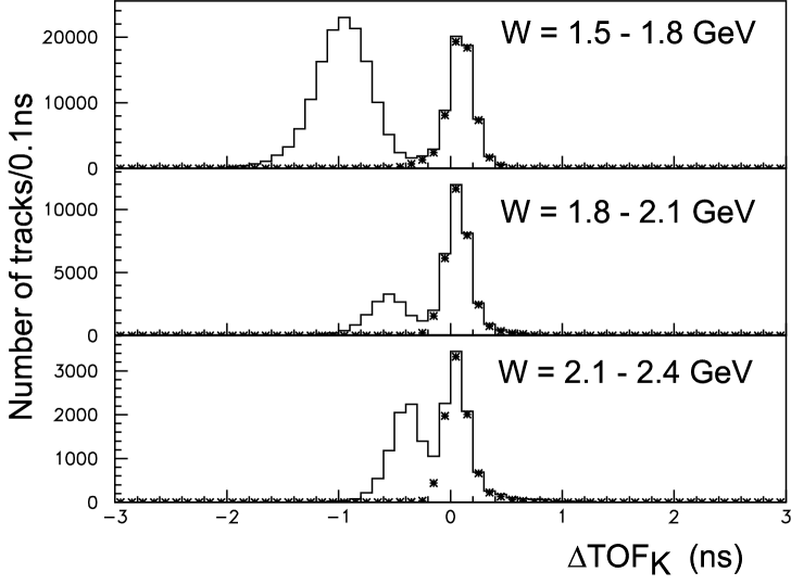
Figure 1: The $\Delta TOF_{K}$ distribution for each track in the event where the other track is identified as a kaon (histogram), and where both tracks are so identified (asterisks), in three different $W$ regions.

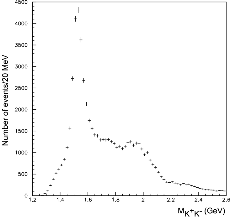
Figure 2: The invariant mass distribution of the $K^{+}K^{-}$ candidates that satisfy all the selection criteria.

4 Derivation of Cross Sections

The cross section for $\gamma\gamma\rightarrow K^{+}K^{-}$ is derived from the present measurement. We restrict the polar-angle range of the final state kaons in the $\gamma\gamma$ c.m. frame ($\theta^{*}$) to be within $|\cos\theta^{*}|<0.6$. The differential cross sections are given by the following formula:

$$\frac{d\sigma}{d|\cos\theta^{*}|}=\frac{\Delta N(W,|\cos\theta^{*}|)~{}(1-f_{\rm BG}(W))}{\int{\mathcal{L}}dt~{}[L_{\gamma\gamma}(W)\Delta W]~{}\Delta|\cos\theta^{*}|~{}\eta(W,|\cos\theta^{*}|)},$$ (1)

where $\Delta N(W,|\cos\theta^{*}|)$ is the number of events in a two-dimensional bin of the c.m. energy ($W$) and the cosine of the polar angle of a meson in the c.m. system ($|\cos\theta^{*}|$) with their widths $\Delta W$ and $\Delta|\cos\theta^{*}|$, respectively, where we take the absolute value of the cosine according to the symmetry of the initial-state particles. In the denominator, $\int{\mathcal{L}}dt$, $L_{\gamma\gamma}(W)$, and $\eta(W,|\cos\theta^{*}|)$ are the integrated luminosity, the luminosity function and the event efficiency at the given kinematical point, respectively.

Residual background due to particle misidentification is corrected using an energy-dependent factor $f_{\rm BG}(W)$, that is derived from a study of the $\Delta TOF_{K}$ distributions shown in Fig. 1. This background fraction is estimated to be less than 3% except in the range 1.55 - 1.65 GeV where it can be as large as 6% due to $f_{2}(1270)\rightarrow\pi^{+}\pi^{-}$ contamination. We neglect any potential $\theta^{*}$ dependence of the correction factor since no prominent angular variation is anticipated in the background that arises mainly from the non-Gaussian tails of the TOF measurements.

The estimated contribution from other background processes, discussed in section 5.3, is much smaller than the total systematic errors (shown in Table 2). We neglect the effect of such backgrounds in the derivation of the cross section.

We use the measured invariant mass of the $K^{+}K^{-}$ system as the $\gamma\gamma$ c.m. energy $W$. The fractional energy resolution $\Delta W/W\simeq 0.2\%$ is estimated from a Monte Carlo (MC) simulation of the signal process (described below). Since this is much smaller than our energy bin size, we neglect smearing across bins in the cross section derivation.

Since we cannot determine the true $\gamma\gamma$ axis in each event, we instead measure $\theta^{*}$ from the direction of the $e^{+}e^{-}$ beam axis in the $e^{+}e^{-}$ c.m. frame. The difference between this and the true polar angle is confirmed to be small using the signal MC simulation, corresponding to an r.m.s. deviation of about 0.015 in $\cos\theta^{*}$.

The efficiency is determined for each bin using the signal MC events for the $e^{+}e^{-}\rightarrow e^{+}e^{-}K^{+}K^{-}$ process that are generated by TREPS [8] and simulated within the Belle detector by a program based on GEANT3 [9]. This efficiency is represented by a smooth function of ($W$, $|\cos\theta^{*}|$) in the analysis.

The trigger efficiency for $K^{+}K^{-}$ events is evaluated separately via a study of detected two-photon $e^{+}e^{-}$ and $\mu^{+}\mu^{-}$ events that satisfy two or more independent trigger conditions. We parameterize the trigger efficiency as a function of the averaged transverse momentum ($\bar{p_{t}}$) of the two tracks in an event. The transverse momentum difference is at most 0.1 GeV/$c$ because of the selection criteria; under these circumstances, the relation $\bar{p_{t}}=\sqrt{(W/2)^{2}-{m_{K}}^{2}}\sin\theta^{*}$ is quite accurate, so the trigger efficiency is calculated by this formula in each ($W$, $|\cos\theta^{*}|$) bin. The laboratory-angle dependence of the trigger efficiency is small within the acceptance range, and we neglect the effect.

The typical value of the efficiency $\eta(W,|\cos\theta^{*}|)$ is 13% at large angles ($|\cos\theta^{*}|<0.3$) in the high-invariant mass region ($W>1.8$ GeV). At most of the other points, it is between 1% and 10%. The large inefficiency seen in $\eta(W,|\cos\theta^{*}|)$ is mainly attributed to detector acceptance effects. The efficiency to identify kaon-pair events within the acceptance is typically 55%, including losses from kaon decays.

We calculate the luminosity function using a separate feature of TREPS [8]. The effects of longitudinal photons are ignored therein. We introduce the form factor effect for finite-$Q^{2}$ photons by multiplying the two-photon flux by the factor $(1+Q_{1}^{2}/W^{2})^{-2}(1+Q_{2}^{2}/W^{2})^{-2}$ in the integrations over $Q_{1}^{2}$ and $Q_{2}^{2}$ for the calculation of the luminosity functions. (Here, $Q_{1}^{2}$ and $Q_{2}^{2}$ are the absolute values of the four-momentum transfer of each photon.) The tight cut of 0.1 GeV/$c$ on $|\sum{\bf p}^{*}_{t}|$ in this analysis limits the uncertainty from the choice of the form factor to less than 2%. The systematic error of the luminosity function is estimated to be 4% by a study that compares the cross sections for the $e^{+}e^{-}\rightarrow e^{+}e^{-}\mu^{+}\mu^{-}$ process using this luminosity function to those from a full $\alpha^{4}$-order QED calculation [10]. The luminosity function $L_{\gamma\gamma}(W)$ and the efficiency $\eta(W,|\cos\theta^{*}|)$ are consistently calculated for two-photon collisions in the same $Q_{1}^{2}$ and $Q_{2}^{2}$ ranges, $Q_{1}^{2}$, $Q_{2}^{2}<1$ GeV². The calculated $L_{\gamma\gamma}(W)$ is a smoothly decreasing function equal to $5.9\times 10^{-3}$ GeV^-1 at $W=1.4$ GeV and $2.0\times 10^{-3}$ GeV^-1 at $W=2.4$ GeV.

The cross section values integrated over $|\cos\theta^{*}|<0.6$ are derived by a binned maximum likelihood fit of the experimental $|\cos\theta^{*}|$ distribution with a bin width of 0.05 carried out at each $W$ bin with a bin width of 0.02 GeV. We assume that the angular dependence of the differential cross section is a second-order polynomial of $\cos^{2}\theta^{*}$ and integrate the fit with $|\cos\theta^{*}|$ between 0 and 0.6. Several data points at $W<1.46$ GeV and $|\cos\theta^{*}|>0.50$ are removed from the fit, where the efficiencies are extremely small.

The obtained cross sections for the process $\gamma\gamma\rightarrow K^{+}K^{-}$ integrated over the range $|\cos\theta^{*}|<0.6$ are summarized in Table 1 and depicted in Fig. 3. The error bars in the figure are statistical only. Systematic errors are tabulated in Table 2, and the dominant sources are described in section 5.

Figure 3 shows our result in comparison with the previous measurements. The errors for our data are statistical only; we note that they are much improved over those of ARGUS [1] and TPC/Two-Gamma [2]. The ARGUS cross sections are obtained for the full angular range ($|\cos\theta^{*}|\leq 1$) by fitting the angular distributions to the sum of two spin-helicity components, $(J,\lambda)=(0,0)$ and $(2,2)$, and should therefore be somewhat larger—typically by 30%—than those of our measurement and TPC/Two-Gamma. (See section 6 for the spin-helicity definition and decomposition.)

Our differential cross sections in the $\gamma\gamma$ c.m. polar angle are plotted in Fig. 4 for each energy bin of width $\Delta W=0.04$ GeV. Again, the displayed errors are statistical only.

Table 1: The cross section of the process $\gamma\gamma\rightarrow K^{+}K^{-}$ in the polar angular region $|\cos\theta^{*}|<0.6$. The first error is statistical and the second systematic.

$W$(GeV)	$\sigma$ ($|\cos\theta^{*}|<0.6$) (nb)
1.40 - 1.42	$5.7\pm 0.7\pm 1.2$
1.42 - 1.44	$5.4\pm 0.7\pm 1.0$
1.44 - 1.46	$5.4\pm 0.5\pm 0.8$
1.46 - 1.48	$7.1\pm 0.3\pm 1.0$
1.48 - 1.50	$10.0\pm 0.2\pm 1.4$
1.50 - 1.52	$14.4\pm 0.3\pm 2.0$
1.52 - 1.54	$14.2\pm 0.3\pm 1.9$
1.54 - 1.56	$11.4\pm 0.2\pm 1.6$
1.56 - 1.58	$7.9\pm 0.2\pm 1.0$
1.58 - 1.60	$5.98\pm 0.15\pm 0.77$
1.60 - 1.62	$4.81\pm 0.13\pm 0.64$
1.62 - 1.64	$4.22\pm 0.12\pm 0.56$
1.64 - 1.66	$3.70\pm 0.11\pm 0.48$
1.66 - 1.68	$3.55\pm 0.11\pm 0.44$
1.68 - 1.70	$3.31\pm 0.11\pm 0.41$
1.70 - 1.72	$3.27\pm 0.10\pm 0.41$
1.72 - 1.74	$3.29\pm 0.11\pm 0.41$
1.74 - 1.76	$3.23\pm 0.10\pm 0.40$
1.76 - 1.78	$3.00\pm 0.10\pm 0.37$
1.78 - 1.80	$2.94\pm 0.10\pm 0.36$
1.80 - 1.82	$2.62\pm 0.09\pm 0.32$
1.82 - 1.84	$2.71\pm 0.09\pm 0.32$
1.84 - 1.86	$2.56\pm 0.09\pm 0.30$
1.86 - 1.88	$2.64\pm 0.09\pm 0.31$
1.88 - 1.90	$2.92\pm 0.09\pm 0.34$
1.90 - 1.92	$2.95\pm 0.09\pm 0.35$
1.92 - 1.94	$2.63\pm 0.08\pm 0.31$
1.94 - 1.96	$2.84\pm 0.09\pm 0.33$
1.96 - 1.98	$2.92\pm 0.10\pm 0.34$
1.98 - 2.00	$2.59\pm 0.09\pm 0.31$
2.00 - 2.02	$2.26\pm 0.08\pm 0.26$
2.02 - 2.04	$2.36\pm 0.08\pm 0.27$
2.04 - 2.06	$1.96\pm 0.08\pm 0.23$
2.06 - 2.08	$1.68\pm 0.07\pm 0.20$
2.08 - 2.10	$1.57\pm 0.07\pm 0.18$
2.10 - 2.12	$1.34\pm 0.06\pm 0.17$
2.12 - 2.14	$1.15\pm 0.06\pm 0.14$
2.14 - 2.16	$0.96\pm 0.06\pm 0.12$
2.16 - 2.18	$0.89\pm 0.06\pm 0.11$
2.18 - 2.20	$0.89\pm 0.06\pm 0.11$
2.20 - 2.22	$0.97\pm 0.06\pm 0.12$
2.22 - 2.24	$0.90\pm 0.06\pm 0.11$
2.24 - 2.26	$0.83\pm 0.06\pm 0.10$
2.26 - 2.28	$0.84\pm 0.06\pm 0.10$
2.28 - 2.30	$0.96\pm 0.06\pm 0.12$
2.30 - 2.32	$0.80\pm 0.05\pm 0.10$
2.32 - 2.34	$0.93\pm 0.06\pm 0.12$
2.34 - 2.36	$0.76\pm 0.06\pm 0.09$
2.36 - 2.38	$0.79\pm 0.06\pm 0.10$
2.38 - 2.40	$0.68\pm 0.06\pm 0.08$

Table 2: The systematic errors for the cross section $\gamma\gamma\rightarrow K^{+}K^{-}$ in the polar angular region $|\cos\theta^{*}|<0.6$. Some systematic errors are $W$-dependent; these are shown as ranges.

	Systematic
Source	error
Trigger efficiency	4 - 6%
Tracking efficiency	4%
$E/p$ cut	4 - 6%
TOF efficiency	3%
Kaon identification efficiency by ACC	0 - 5%
$t_{0}$ ambiguity	0 - 7%
Acceptance calculation	3 - 15%
Particle misidentification backgrounds	1 - 2%
Non-exclusive backgrounds	4 - 6%
Integrated luminosity	1%
Luminosity function and form-factor effect	4%
Total	11 - 20%

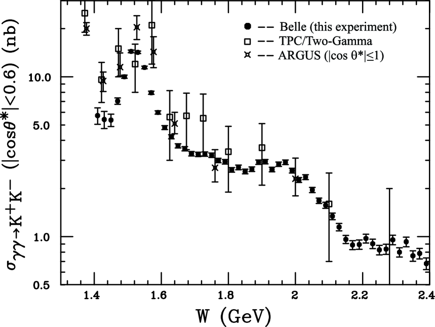
Figure 3: The cross section for $\gamma\gamma\rightarrow K^{+}K^{-}$ in the polar angular region $|\cos\theta^{*}|<0.6$ obtained in this experiment compared with results from previous experiments [1,2]. The error bars are statistical only.

Figure 4: The differential cross section $d\sigma/d|\cos\theta^{*}|$ for $\gamma\gamma\rightarrow K^{+}K^{-}$ obtained in this experiment. The solid curves are the fits described in section 6.2. The error bars are statistical only.

5 Major sources of systematic error

5.1 Trigger efficiency

We determine the trigger efficiency for the $K^{+}K^{-}$ final samples that would pass all the selection criteria described in section 3. We first estimate the efficiency of the two-track trigger, which requires two or more TOF/TSC hits as well as one or more CsI clusters. The efficiency is determined experimentally as a function of transverse momentum between 0.4 and 1.2 GeV/$c$, using the redundancy of triggers for two-photon $e^{+}e^{-}$ and $\mu^{+}\mu^{-}$ events. The ratio of the yield from this particular trigger to that from all the trigger sources —typically 0.88— is used to determine the overall trigger efficiency. We confirm that there is no notable explicit dependence of the trigger efficiency on the polar angle in the laboratory system. The results on the trigger efficiency are compared with those from our trigger simulation program, which is applied immediately after the full detector simulation. The simulation reproduces a quantitative nature of the $p_{t}$ dependence of the trigger efficiency. Although the trigger efficiency value from the simulation is not used for the cross section calculations, the difference between experimental and MC values is taken into account in the systematic error. A small difference between the trigger efficiency for leptons and hadrons estimated from the experimental and simulation studies is applied as a correction and included to the systematic error as well. The trigger efficiency thus determined is $(82\pm 5)\%$ at $\bar{p_{t}}=0.55$ GeV/$c$ and $(92\pm 4)\%$ at $\bar{p_{t}}=1.0$ GeV/$c$.

The samples after application of the event selection criteria before particle identification are used for a confirmation of the trigger efficiency. We have compared the experimental yields of these samples in the $W$ and laboratory polar angle distributions to the expectations from the MC calculation. Those samples are dominated by $e^{+}e^{-}\rightarrow e^{+}e^{-}e^{+}e^{-}$, $e^{+}e^{-}\mu^{+}\mu^{-}$ and $e^{+}e^{-}\pi^{+}\pi^{-}$ processes whose cross sections are well known [10, 11, 12]. The experimental and MC yields are consistent within the above error of the trigger efficiency.

5.2 Kaon-identification efficiency

We have checked the kaon-identification efficiency in this analysis based on the real data. The efficiency to identify and select kaon-pair events within the detector acceptance is typically 55%. The 45% loss is partially due to kaon decays, which account for 20-30% depending on the two kaon invariant mass. An additional reduction of $\sim 25$% comes from the kaon identification criteria for the TOF, ACC and $E/p$ requirements.

The efficiency of the TOF counters giving a useful TOF measurement for a track, which is required in the kaon selection, is obtained using the events in which the other track is tagged as a kaon. The efficiency thus obtained in the real data is around 92% in the $0.5<p<1.0$ GeV/$c$ region where the signal events dominate, comparable to the MC simulation’s efficiency of 94% at around 1 GeV/$c$. The effect of a trigger efficiency loss due to kaon decays is small in this comparison. We take the difference of the TOF efficiency between the experimental and MC data, 3% for the two tracks, as a systematic error.

The efficiency of kaon-pair identification in the offline selection is examined using the redundancy of two kaons in a signal $K^{+}K^{-}$ event. The $\Delta TOF_{K}$ distribution for a track is investigated for events where the other track is identified as a kaon as shown in Fig. 1. We find that charged tracks whose $\Delta TOF_{K}$ is consistent with a kaon are identified as a kaon with an efficiency higher than 95%; this value is consistent with the MC expectation within the systematic error of 5% or less in all $W$ regions.

The $E/p$ cut gives an inefficiency in kaon selection as a nuclear interaction of a negative kaon in the ECL sometimes gives a large energy deposition. We compared the fractions of kaons with $E/p>0.8$ to those with any $E/p$ between the MC events and real $K^{+}K^{-}$ samples; they are consistent. A small possible discrepancy ($\sim 6\%$ at $W<1.8$ GeV and $\sim 4\%$ at $W>1.8$ GeV) is accounted for in the systematic error.

5.3 Backgrounds from particle misidentification and non-
exclusive events

The correction factor for the background contamination from particle misidentification is evaluated from the study of the experimental data, as described in section 4. Another study using the MC expectations from the $e^{+}e^{-}e^{+}e^{-}$, $e^{+}e^{-}\mu^{+}\mu^{-}$ [10] and $e^{+}e^{-}\pi^{+}\pi^{-}$ processes [11, 12], which dominate this kind of background, is also consistent with this evaluation. We assign a systematic error of 1-2% from this source, depending on $W$. This background source has no effect on the significance of the resonant structures that are observed in the $K^{+}K^{-}$ spectrum and discussed in this paper.

We also estimate the background contamination from events where additional particles accompany the two detected tracks—so-called non-exclusive backgrounds. Such events are expected to give a larger $|\sum{\bf p}^{*}_{t}|$ than the signal events. Figure 5 shows the distribution of $|\sum{\bf p}^{*}_{t}|$ for the $K^{+}K^{-}$ signal candidates, with the simulated distribution scaled to match the data yield in the first two bins. The data and signal MC show generally good agreement over the entire accepted range of $|\sum{\bf p}^{*}_{t}|$, and we conclude that the backgrounds from non-exclusive processes are small. The small difference between the experimental and MC distributions seen at high $|\sum{\bf p}^{*}_{t}|$ may be attributed to the non-exclusive backgrounds (or any other process that does not have an enhancement at zero-$p_{t}$ balance).

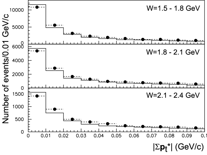
Figure 5: The transverse momentum balance ($|\sum{\bf p}^{*}_{t}|$) distribution for the signal process from the real data (closed circles) and signal MC events (histogram) for events in three $W$ regions. The MC distributions are scaled to match the data yield in the first two bins.

We find that the contamination of such background processes is less than 6% at any $W$, based on the expectation that the background contribution vanishes at $|\sum{\bf p}^{*}_{t}|=0$ and the assumption that the observed surplus over MC expectation in the rightmost bin of Fig. 5 is purely from the contribution from the non-exclusive background. In the experimental data, a larger excess over the MC expectation is seen at $|\sum{\bf p}^{*}_{t}|$ around 0.01 - 0.04 GeV/$c$. This excess cannot be attributed to the non-exclusive backgrounds, and is considered to be due to an unmodelled broadening of the signal-process distribution.

It is difficult to determine the magnitude of these backgrounds, so we neglect their effect in the derivation of cross sections and instead account for them in the systematic error.

6 Phenomenological analyses

6.1 The c.m.-energy dependence

The obtained $\gamma\gamma$ c.m.-energy dependence of the experimental yield (Fig. 2) and the cross section (Fig. 3) clearly show four resonant structures, in the vicinities of 1.52 GeV, 1.7 - 1.8 GeV, 1.9 - 2.1 GeV, and 2.2 - 2.4 GeV. The peak near 1.52 GeV is from the $f^{\prime}_{2}(1525)$ resonance, which is considered to be a ground-state tensor meson dominated by an $s\bar{s}$ component. The contribution of this resonance in this reaction is well known from previous measurements [1, 2]. In contrast, this measurement constitutes the first observation of the other three structures.

The $W$ dependence of the cross section is fitted to a sum of contributions from resonances and a continuum component. The components adopted in the fit are: (A) the $f^{\prime}_{2}(1525)$ resonance, (B) a resonance around 1.75 GeV, (C) a resonance around 2.0 GeV, (D) a resonance around 2.3 GeV, (E) contributions from the continuum component and the tails of two low-mass resonances, $f_{2}(1270)$ and $a_{2}(1320)$. For (A)–(D), we use an amplitude with a relativistic Breit-Wigner form:

$${\mathcal{A}}_{R}=\frac{\sqrt{S\Gamma}}{W^{2}-M^{2}-iM\Gamma},$$ (2)

where $S$, $M$ and $\Gamma$ are the size parameter, mass and total width of the resonance, respectively. The component (E) is expressed by an amplitude with a $W$-dependent form and three free parameters $a$, $b$, and $W_{0}$ as

$${\mathcal{A}}_{E}=a(\frac{W-W_{0}}{1.4~{}{\rm GeV}-W_{0}})^{-b},$$ (3)

where we combine the effects from the tails of the low-mass resonances and the smooth continuum since we cannot decompose these effects in our present measurement. The interference phases between (A) and (E) and between (C) and (E) are treated as free parameters. (B) and (D) are considered incoherent since  their  peaks  are  relatively  small and  it is  difficult to  determine  the  relative  phase. For  the  $f^{\prime}_{2}(1525)$  resonance,  the  $W$-dependent  total  width  is $\Gamma(W)=\Gamma_{M}(p^{*}/p_{0}^{*})^{5}(M/W)(D_{2}(p^{*}r)/D_{2}(p_{0}^{*}r))$, where $M$ and $\Gamma_{M}$ are the nominal mass and total width, respectively, while $p^{*}$ and $p_{0}^{*}$ are the momenta of the final-state kaon in the rest frame of the resonance with invariant mass $W$ and $M$, respectively. The function $D_{2}(z)\sim(9+3z^{2}+z^{4})^{-1}$ [13] represents a centrifugal barrier factor; we use an effective interaction radius of $r=1$ fm. We use $W$-independent total widths for the other three resonances. We denote the $\Gamma_{M}$ for the $f_{2}^{\prime}(1525)$ simply by $\Gamma$ in the remainder of this paper.

The result of the fit is summarized in Table 3. The curves in Fig. 6 show the fit and the contribution from each component superimposed on the experimental data. The goodness of fit is $\chi^{2}/{\rm ndf}=50.8/33$. We use only statistical errors for this calculation and its minimization. We determine the systematic errors of the fitted parameters by a study of their changes for four cases of linear deformations of the measured cross section as a function of $W$.

Table 3: Resonance parameters and other variables obtained from the fit of the $W$ dependence of the cross section. The first error is statistical and the second systematic.

Resonance		Mass	Total width	$S$	Signi-
components		(MeV/$c^{2}$)	(MeV)	(nb GeV3)	ficance
(A)	($f_{2}^{\prime}(1525)$)	$1518\pm 1\pm 3$	$82\pm 2\pm 3$	$1.22\pm 0.11\pm 0.25$	$>25\sigma$
(B)	(1.75 GeV)	$1737\pm 5\pm 7$	$151\pm 22\pm 24$	$0.45\pm 0.09\pm 0.10$	$5.5\sigma$
(C)	(2.0 GeV)	$1980\pm 2\pm 14$	$297\pm 12\pm 6$	$2.63\pm 0.11\pm 0.57$	$>9\sigma$
(D)	(2.3 GeV)	$2327\pm 9\pm 6$	$275\pm 36\pm 20$	$0.94\pm 0.13\pm 0.28$	$5.3\sigma$
(E)		$a=2.12\pm 0.17\pm 0.54$ nb1/2,
		$W_{0}=0.04\pm 0.02\pm 0.33$ GeV, $b=7.9\pm 1.0\pm 2.0$
Interference		${\rm(A)}-{\rm(E)}:-1.27\pm 0.07\pm 0.12$ rad
phases		${\rm(C)}-{\rm(E)}:+2.57\pm 0.14\pm 0.38$ rad

The small confidence level of the $\chi^{2}/{\rm ndf}$ value is attributed to the inability of our fit function to reproduce faithfully the true behavior of the cross section rather than any systematic-error effects; nevertheless, we expect that we can obtain meaningful resonance parameters by this parametrization. We note that there could be additional systematic shifts in the parameters for the particular resonant structure at 2.3 GeV due to the boundary of our available $W$ range, $W<2.4$ GeV.

The statistical significances for the resonant structures are also given in the last column of Table 3, They are derived from the square root of the goodness of fit difference between the fits with and without the corresponding resonance components for the structures at 1.75 GeV and 2.3 GeV. Each of the other two structures dominates the cross section in its energy region, and this technique is not suitable to estimate the significance. We show, instead, the significances for the excess of the core part of the peak that appears above the averaged level of whole the apparent peak structure, regarding the deviation from the level as the corresponding lower limit.

The component (E) gives a significant contribution only at $W<1.7$ GeV in the above fit. An alternative form for (E) with two summed amplitudes having distinct tail decay parameters did not yield an improved goodness of fit nor a substantial change in the overall shape of the (E) component and the values of the other resonance parameters. We conclude that the cross section at energies above 1.7 GeV is dominated by the contribution from the four resonances that appear in our fit.

We note that the size parameter $S$ is proportional to the product $\Gamma_{\gamma\gamma}(R){\mathcal{B}}(R\rightarrow K^{+}K^{-})$ of the resonance and depends on its spin $J$ and helicity $\lambda$ along the $\gamma\gamma$ axis as:

$$S=8\pi(2J+1)F~{}\Gamma_{\gamma\gamma}(R){\mathcal{B}}(R\rightarrow K^{+}K^{-}),$$ (4)

$$F=(2J+1)\sum_{\lambda=0,2}f_{\lambda}\int_{0}^{0.6}[d^{J}_{\lambda,0}(z)]^{2}dz.$$ (5)

$F$ corresponds to the fraction of the resonance component’s cross section integrated over $|\cos\theta^{*}|<0.6$ to the total, while $f_{\lambda}$ is the fraction of the resonance production rate in the $\lambda$ helicity state (with $f_{0}+f_{2}=1$). The integrands in Eq. (5) are the square of the factors of the Wigner $D$-functions. For a $J=0$ meson, only $\lambda=0$ is allowed so that $F=0.6$. We discuss the extraction of $\Gamma_{\gamma\gamma}(R){\mathcal{B}}(R\rightarrow K^{+}K^{-})$ from this analysis in section 7.

Figure 6: The measured cross section of the process $\gamma\gamma\rightarrow K^{+}K^{-}$ in the polar angular region $|\cos\theta^{*}|<0.6$, compared with the fit described in section 6.1. The error bars are statistical only. The solid curve indicates the best fit. The dotted curve and four dashed curves indicate the contributions from component (E) and from the four resonance components, respectively, without interference. The dot-dashed curve is the contribution of the interference term.

6.2 Angular dependence

The angular dependence of the differential cross section has an enhancement at large angles (near $|\cos\theta^{*}|=0$) for the lower values of $W$, but has a tendency of a forward enhancement at the higher $W$ values. The dependence is almost flat in the vicinity of 2.3 GeV. We first plot the ratio of cross sections over the restricted range $|\cos\theta^{*}|<0.3$ and the measured range ($|\cos\theta^{*}|<0.6$):

$$R=\frac{\int_{0}^{0.3}\frac{d\sigma}{d|\cos\theta^{*}|}d|\cos\theta^{*}|}{\int_{0}^{0.6}\frac{d\sigma}{d|\cos\theta^{*}|}d|\cos\theta^{*}|}$$ (6)

to draw out this gross behavior of the angular distribution. The $W$ dependence of this ratio is plotted in Fig. 7 for $W$ points above 1.46 GeV, where we have complete angular data over the range $|\cos\theta^{*}|<0.6$. It has a large value at around 1.5 GeV and 2.0 GeV, respectively. These positions correspond to the two larger resonant structures designated (A) and (C) in section 6.1.

We make a model-independent angular analysis for the angular distribution of the $K^{+}K^{-}$ events. The angular distribution is fitted by the sum of the partial-wave contributions, independently at each $W$ bin. For the total angular momentum ($J$) of the $\gamma\gamma$ system, we assume that the partial waves with $J\geq 4$ are negligible. The odd-$J$ waves are forbidden by the symmetric nature of the initial state and parity conservation. In the $\gamma\gamma$ c.m. system, the differential cross section can be written as

$$\frac{d\sigma}{d\Omega}=|{\mathcal{H}}(0,0)+{\mathcal{H}}(2,0)|^{2}+|{\mathcal{H}}(2,2)|^{2}$$ (7)

where ${\mathcal{H}}(J,\lambda)$ is the partial-wave amplitude for the (spin, helicity)=($J$, $\lambda$) state, and $\Omega$ is the solid angle.

Equation (7) includes four real parameters—the sizes of the three partial-wave amplitudes and one relative phase between the two $\lambda=0$ waves—while only three are determined independently by this measurement. (This formula is a quadratic function of $\cos^{2}\theta^{*}$.) Thus, we choose an alternative parameterization as follows. With $\sigma_{J\lambda}=\int|{\mathcal{H}}(J,\lambda)|^{2}d\Omega$ as the positive definite squared partial wave amplitude over the whole solid angle, we parameterize the differential cross section in terms of three cross section-like parameters $\sigma_{a}$, $\sigma_{b}$, and $\sigma_{c}$ and the factors of the Wigner $D$-functions as [12]

$$\frac{d\sigma}{d|\cos\theta^{*}|}=\sigma_{a}+5\sigma_{b}\{d^{2}_{0,0}(\cos\theta^{*})\}^{2}+5\sigma_{c}\{d^{2}_{2,0}(\cos\theta^{*})\}^{2}.$$ (8)

The coefficients $\sigma_{a}$, $\sigma_{b}$ and $\sigma_{c}$ coincide with $\sigma_{00}$, $\sigma_{20}$ and $\sigma_{22}$, respectively, if there is no interference between the two $\lambda=0$ components. When we account for this interference, the correspondence is modified [12]:

$$\sigma_{a} = \sigma_{00}+s_{I}$$ (9)

$$\sigma_{b} = \sigma_{20}+\frac{1}{5}s_{I}$$ (10)

$$\sigma_{c} = \sigma_{22}-\frac{6}{5}s_{I}$$ (11)

$$s_{I} = \sqrt{5\sigma_{00}\sigma_{20}}\cos\psi,$$ (12)

where $\psi$ is the relative phase between the interfering amplitudes ${\mathcal{H}}(0,0)$ and ${\mathcal{H}}(2,0)$ that we cannot determine independently. We note that $\sigma_{a}$, $\sigma_{b}$ and $\sigma_{c}$ can be negative in the presence of this interference.

The fit values for $\sigma_{a}$, $\sigma_{b}$ and $\sigma_{c}$ in each $W$ bin are summarized in Fig. 8. The corresponding fit curves are shown in Fig. 4, which indicates a good parametrization of the measured magnitude and polar angular dependence.

In the fits, we constrain the best-fit values of $\sigma_{a}$, $\sigma_{b}$, and $\sigma_{c}$ to give a non-negative differential cross section throughout the full angular range, $|\cos\theta^{*}|\leq 1$. Only the fit to the lowest-energy bin, at $W=1.40$ - 1.44 GeV, is affected by this constraint ($d\sigma/d|\cos\theta^{*}|=0$ near $|\cos\theta^{*}|=0.67$).

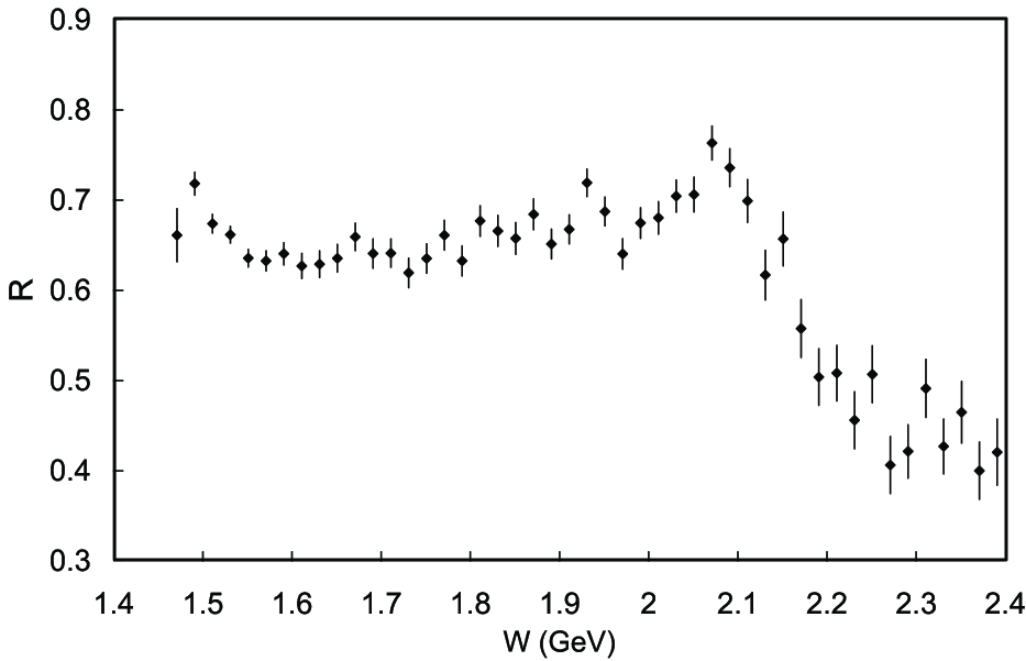
Figure 7: The $W$ dependence of $R$, the ratio of the cross sections in the angular ranges $|\cos\theta^{*}|<0.3$ and $|\cos\theta^{*}|<0.6$.

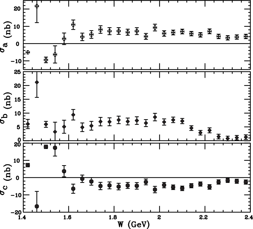
Figure 8: The solution for the partial-wave coefficients $\sigma_{a}$ (top), $\sigma_{b}$ (middle), and $\sigma_{c}$ (bottom).

7 Discussion

7.1 $f_{2}$’(1525)

The resonance parameters obtained by the present measurement are summarized and compared with those from previous experiments in Table 4.

Our best fit mass and total width of $f^{\prime}_{2}(1525)$ are in agreement with those from previous experiments [4]. In the range 1.5 - 1.6 GeV, the parameter $\sigma_{c}$ has a large peak. This feature is consistent with the previous determination that the $f^{\prime}_{2}(1525)$ is a spin-2 meson. We confirm that its production in two-photon collisions is dominated by the $\lambda=2$ helicity component.

From each size parameter $S$, we extract $\Gamma_{\gamma\gamma}(R){\mathcal{B}}(R\rightarrow K^{+}K^{-})$ for the corresponding resonance $R$ of assigned spin and helicity using Eqs. (4) and (5). These results are also shown in Table 4. Their systematic errors are simply scaled from those in $S$; they do not incorporate any effects from the assumptions in resonance formulae, background shapes and interference effects.

When we assume a pure $(J,\lambda)=(2,2)$ state for $f^{\prime}_{2}(1525)$, we obtain $\Gamma_{\gamma\gamma}(f^{\prime}_{2}){\mathcal{B}}(f^{\prime}_{2}\\ \rightarrow K^{+}K^{-})=28.2\pm 2.4\ {\rm(stat.)}\pm 5.8\ \rm{(syst.)}$ eV. This result is slightly smaller than the world average [4] (where isospin invariance is assumed) but is still larger than the ARGUS result where the interference effect is taken into account [1].

We note that our systematic error does not account fully for the ambiguity in the interference effect with the low-lying resonances $f_{2}(1270)$ and $a_{2}(1320)$, since this effect cannot be clarified by the present data alone. We have tried an alternative fit where the mass, width and size parameters of the $f_{2}(1270)$ and $a_{2}(1320)$ are fixed to their accepted values [4] and they are assumed to interfere with a zero relative phase; the quality of this fit is poor and the cross section is significantly larger than the present measurement in the mass region of the $f^{\prime}_{2}(1525)$.

7.2 The structure around 2.0 GeV

We see a broad resonant structure around $W=2.0$ GeV in the cross section. However, there is no remarkable structure in the individual $\sigma_{a}$, $\sigma_{b}$ and $\sigma_{c}$ distributions near 2.0 GeV, nor in the total cross section $\sigma_{\rm tot}=\sigma_{a}+\sigma_{b}+\sigma_{c}$ (wherein the interference term $s_{I}$ drops out). An apparent lack of consistency between this situation and the $W$-dependence of the measured cross section arises mainly from the fact that the variation of the parameter $\sigma_{b}$ dominates the feature of $\sigma_{\rm tot}$ with its large contribution at small angles and conceals effects of the $\sigma_{c}$ contribution, which is enhanced only at large angles.

Our fit gives negative values of $\sigma_{c}$ in the wide $W$ region above 1.6 GeV. This feature might imply a non-negligible (negative) interference contribution ($s_{I}$) and, therefore, sizable values for both $\sigma_{00}$ and $\sigma_{20}$. Given the expected dominance of only the ${\mathcal{H}}(2,2)$ component in tensor-meson production, we still cannot explain the relatively narrow enhancement around $|\cos\theta^{*}|=0$ in the angular dependence for $W$ between 1.8 and 2.1 GeV.

Thus, no conclusive result is obtained for the spin of the structure near 2.0 GeV from our angular analysis. However, the large $R$ value near 2.0 GeV shown in Fig. 7 indicates that an assignment of $J=2$ is qualitatively favored for this resonance, since both $|{\mathcal{H}}(2,0)|^{2}$ and $|{\mathcal{H}}(2,2)|^{2}$ have a peak at $\cos\theta^{*}$ = 0.

Our best fit mass and total width of the resonant structure near 2.0 GeV match those tabulated for the $f_{2}(2010)$ meson [4]. We obtain $\Gamma_{\gamma\gamma}{\mathcal{B}}=61\pm 2\pm 13$ eV for the assumption of $(J,\lambda)=(2,2)$. This result is similar in scale to that of $f_{2}^{\prime}(1525)$ and supports the hypothesis that this resonance is a $q\bar{q}$ meson with a sizable $s\bar{s}$ component [14, 15].

Table 4: Resonance parameters from the results of this study compared to relevant previous measurements. $M$ and $\Gamma$ are the mass and the total width of the resonance in units of MeV/$c^{2}$ and MeV, respectively, and $\Gamma_{\gamma\gamma}{\mathcal{B}}$ is the product of the two-photon decay width and the branching fraction to the $K^{+}K^{-}$ final state for the resonance ($\Gamma_{\gamma\gamma}(R){\mathcal{B}}(R\rightarrow K^{+}K^{-})$) in units of eV. For the present measurement, $\Gamma_{\gamma\gamma}{\mathcal{B}}$ is derived from the $S$ values for the stated $(J,\lambda)$ hypothesis. For prior observations (cited in the rightmost column), isospin invariance is assumed for comparison with our results, and any additional notes are given at the bottom of the table.

Reson-	The present		Other possibly
ance	measurement		relevant observations
$f_{2}^{\prime}(1525)$	$M$:	$1518\pm 1\pm 3$	$f_{2}^{\prime}(1525)$	$M$:	$1525\pm 5$	[4]
	$\Gamma$:	$82\pm 2\pm 3$		$\Gamma$:	$76\pm 10$
	$\Gamma_{\gamma\gamma}{\mathcal{B}}$:	$28.2\pm 2.4\pm 5.8$		$\Gamma_{\gamma\gamma}{\mathcal{B}}$:	$40\pm 4.5$
		((2,2) assumed)		$\Gamma_{\gamma\gamma}{\mathcal{B}}$:	$15.7\pm 2.5\pm 3.9^{1)}$	[1]
1.75 GeV	$M$:	$1737\pm 5\pm 7$	$f_{J}(1710)^{2)}$	$M$:	$1767\pm 14$	[3]
	$\Gamma$:	$151\pm 22\pm 24$		$\Gamma$:	$187\pm 60$
	$\Gamma_{\gamma\gamma}{\mathcal{B}}$:	$10.3\pm 2.1\pm 2.3$		$\Gamma_{\gamma\gamma}{\mathcal{B}}$:	$24.5\pm 5.5\pm 6.5$
		((2,2) assumed)	$f_{0}(1710)$	$M$:	$1713\pm 6$	[4]
		$76\pm 15\pm 17$		$\Gamma$:	$125\pm 10$
		((0,0) assumed)	$a_{2}(1750)$	$M$:	$1752\pm 21\pm 4$	[16]
				$\Gamma$:	$150\pm 110\pm 34$
			$a_{2}(1700)$	$M$:	$1726\pm 26$	[4]
				$\Gamma$:	$256\pm 40$
2.0 GeV	$M$:	$1980\pm 2\pm 14$	$f_{2}(2010)$	$M$:	$2011^{+62}_{-76}$	[4]
	$\Gamma$:	$297\pm 12\pm 6$		$\Gamma$:	$202^{+67}_{-62}$
	$\Gamma_{\gamma\gamma}{\mathcal{B}}$:	$61\pm 2\pm 13$
		((2,2) assumed)
2.3 GeV	$M$:	$2327\pm 9\pm 6$	$f_{J}(2220)$	$M$:	$2231.1\pm 3.5$	[4]
	$\Gamma$:	$275\pm 36\pm 20$		$\Gamma$:	$23^{+8}_{-7}$
	$\Gamma_{\gamma\gamma}{\mathcal{B}}$:	$22\pm 3\pm 6$	$f_{2}(2300)$	$M$:	$2297\pm 28$	[4]
		((2,2) assumed)		$\Gamma$:	$149\pm 41$
		$161\pm 22\pm 48$
		((0,0) assumed)

The units of $M$, $\Gamma$, and $\Gamma_{\gamma\gamma}{\mathcal{B}}$ are MeV/$c^{2}$, MeV, and eV, respectively.

¹⁾ Using a coherent background.
              ²⁾ Spin 2 is reported to be dominant in the measurement [3].

7.3 The structures around 1.75 GeV and 2.3 GeV

Our best fit mass and width of the resonance structure at 1.75 GeV in our data are compatible with the corresponding values of a resonance in ref. [3] that the authors associate with $f_{J}(1710)$ in their measurement of $\gamma\gamma\rightarrow K_{S}^{0}K_{S}^{0}$. These numbers are excluded from the latest world-average values [4] of the $f_{0}(1710)$ since ref. [3] favors a spin assignment of $J=2$ while ref. [4] has assigned it $J=0$. The measurement of the $\pi^{+}\pi^{-}\pi^{0}$ final-state production from two-photon collisions [16] also finds a resonance near 1.75 GeV with a mass and width close to our values (they are shown as $a_{2}(1750)$ in Table 4). Ref. [4] cites this resonance as $a_{2}(1700)$, with a world-average value that includes ref. [16] as well as results from hadron-beam experiments.

We cannot determine the spin-helicity of this structure from the present analysis alone, since the fraction of its contribution to the total cross section is small. The isospin of the resonant structure also can not be determined from the present experiment only. However, the difference in resonant structures between the $K^{+}K^{-}$ and $K^{0}_{S}K^{0}_{S}$ channels, where in the latter process no enhancement near 2.0 GeV is seen [3], can be naively explained by distinct interference effects of two or more resonances having different isospins. Along this line, interference between $I=0$ and $I=1$ mesons—$f$ and $a$ mesons, respectively—is a plausible explanation for the contrasting behavior between the $K^{+}K^{-}$ and $K^{0}_{S}K^{0}_{S}$ channels between 1.6 and 2.1 GeV.

As noted earlier, the angular distribution is rather flat near $W=2.3$ GeV. However, it is not clear that this is due to a spin property of the resonance we find in this mass region, since the observed evolution of the angular dependence with energy may come from the effect of hard parton scatterings, which have a tendency of giving a forward enhancement at high energies.

In fact, the feature of the negative $\sigma_{c}$ in $W>1.6$ GeV, mentioned in the previous subsection, may be simply an artifact of our having neglected the partial waves of $J\geq 4$, for example, due to hard scatterings with partons, which cause an enhancement at forward angles (corresponding to high-$J$ waves) at these higher energies. Our fit compensates for the omission of any $J\geq 4$ partial waves with a negative (positive) offset in $\sigma_{c}$ ($\sigma_{b}$). We get reasonable fits of the angular distributions for $W>2.2$ GeV with a sum of incoherent amplitudes, $|{\mathcal{H}}({\rm QCD})|^{2}+|{\mathcal{H}}(2,2)|^{2}$, where we assume $|{\mathcal{H}}({\rm QCD})|^{2}$ has an angular dependence proportional to $\sin^{-4}\theta^{*}$ [17]. Then, the drastic change of the angular distribution observed at 2.1 - 2.3 GeV provides very important information about the perturbative-QCD nature of this process.

We cannot find any evidence of a narrow-width structure corresponding to the glueball candidate $f_{J}(2220)$ that is reported in the radiative decays of $J/\psi$ near 2.23 GeV [5] with $\Gamma<30$ MeV. However, this narrow width is not well established, so it is possible that a part of the wide structure that we see in this mass region comes from the $f_{J}(2220)$. We note that the identity of $f_{J}(2220)$ in relation with other resonances in the same mass region—$f_{2}(2300)$ and $f_{4}(2300)$, for example—is not yet clarified.

Our size parameter $S$ for the resonant structure gives $\Gamma_{\gamma\gamma}{\mathcal{B}}=22\pm 3\pm 6$ eV for the spin-helicity hypothesis of $(J,\lambda)=(2,2)$. This does not contradict the upper limit value for $f_{J}(2220)$ obtained from previous two-photon measurements — for example, the 95% C.L. upper limit for the $K^{0}_{S}K^{0}_{S}$ channel [18] is $\Gamma_{\gamma\gamma}(f_{J}(2220)){\mathcal{B}}(f_{J}(2220)\rightarrow K^{0}_{S}K^{0}_{S})<1.0$ eV for a pure $(2,2)$ assumption—since those analyses assume a narrow width of $\Gamma(f_{J}(2220))=20$ - 30 MeV. Our analysis prefers a width about ten times larger.

Working with the hypothesis of a narrow-width $f_{J}(2220)$, we extract an upper limit for its $\Gamma_{\gamma\gamma}{\mathcal{B}}$ by fixing its mass and width at 2231 MeV/$c^{2}$ and 23 MeV, respectively [4], and assuming pure $(J,\lambda)=(2,2)$ production. We fit the invariant-mass distribution of the signal events in $|\cos\theta^{*}|<0.6$ with a sum of a second order polynomial plus a Breit-Wigner function in the mass range between 2.13 and 2.33 GeV/$c^{2}$. We see no significant excess from the smooth polynomial level. Our 95% C.L. upper limit is $\Gamma_{\gamma\gamma}(f_{J}(2220)){\mathcal{B}}(f_{J}(2220)\rightarrow K^{+}K^{-})<0.60$ eV, corresponding to a fit including this resonance whose $\chi^{2}$ exceeds that of the best fit by $(1.64)^{2}$. We account for the systematic error in the measurement by inflating the upper limit by $1\sigma$ of the total systematic error. This limit is an improvement on the value from the $K^{0}_{S}K^{0}_{S}$ measurement which is cited from ref. [18] in the previous paragraph, assuming we can compare the two by isospin invariance.

8 Conclusion

The production of $K^{+}K^{-}$ in two-photon collisions has been studied using a 67 fb^-1 data sample. The $\gamma\gamma$ center of mass energy dependence of the cross section for the process $\gamma\gamma\rightarrow K^{+}K^{-}$ is measured in the range 1.4 - 2.4 GeV with much higher statistical precision than was achieved previously.

A clear peak for $f^{\prime}_{2}(1525)$ is observed, as reported by prior experiments. We find three new resonant structures in the vicinities of 1.75 GeV, 2.0 GeV and 2.3 GeV, respectively. The mass, width and size parameters for these resonant structures have been obtained from the fit of the energy dependence of the cross section.

The structure around 2.0 GeV has sizeable contribution to the cross section, and the angular distribution has a large-angle enhancement in this mass region.

The angular dependence of the differential cross section has a drastic change at 2.1 - 2.3 GeV; below this energy, the differential cross section is more enhanced at large angles, and it is more enhanced at small angles above this energy.

We do not find any signature of a narrow ($\Gamma<30$ MeV) structure in the vicinity of 2.23 GeV.

We hope some questions raised by this paper will be clarified by further data processing as well as combined analysis of different final states. On the other hand, better phenomenological models taking into account the interfering resonances together with QCD nonresonant contributions are certainly needed.
 
 

Acknowledgements
We wish to thank the KEKB accelerator group for the excellent operation of the KEKB accelerator. We acknowledge support from the Ministry of Education, Culture, Sports, Science, and Technology of Japan and the Japan Society for the Promotion of Science; the Australian Research Council and the Australian Department of Education, Science and Training; the National Science Foundation of China under contract No. 10175071; the Department of Science and Technology of India; the BK21 program of the Ministry of Education of Korea and the CHEP SRC program of the Korea Science and Engineering Foundation; the Polish State Committee for Scientific Research under contract No. 2P03B 01324; the Ministry of Science and Technology of the Russian Federation; the Ministry of Education, Science and Sport of the Republic of Slovenia; the National Science Council and the Ministry of Education of Taiwan; and the U.S. Department of Energy.

References

- [1] ARGUS Collaboration, H. Albrecht et al., Z. Phys. C48, 183 (1990).
- [2] TPC/Two-Gamma Collaboration, H. Aihara et al., Phys. Rev. Lett. 57, 404 (1986).
- [3] L3 Collaboration, M. Acciarri et al., Phys. Lett. B501, 173 (2001).
- [4] Particle Data Group, K. Hagiwara et al., Phys. Rev. D66, 010001 (2002).
- [5] BES Collaboration, J.Z. Bai et al., Phys. Rev. D68, 052003 (2003); BES Collaboration, J.Z. Bai et al., Phys. Rev. Lett. 76, 3502 (1996); BES Collaboration, J.Z. Bai et al., Phys. Rev. Lett. 77, 3959 (1996); Mark III Collaboration, R.M. Baltrusaitis et al., Phys. Rev. Lett. 56, 107 (1986).
- [6] Belle Collaboration, A. Abashian et al., Nucl. Instr. Meth. A479, 117 (2002).
- [7] S. Kurokawa and E. Kikutani, Nucl. Instr. Meth. A499, 1 (2003).
- [8] S. Uehara, KEK Report 96-11 (1996).
- [9] R. Brun et al., CERN DD/EE/84-1 (1987).
-
[10]
F.A. Berends, P.H. Daverveldt and R. Kleiss, Nucl. Phys. B253, 441 (1985);
F.A. Berends, P.H. Daverveldt and R. Kleiss, Comp. Phys. Comm. 40, 285 (1986). -
[11]
Mark II Collaboration, J.H. Boyer et al., Phys. Rev. D42, 1350 (1990);
CELLO Collaboration, H.-J. Behrend et al., Z. Phys. C56, 381 (1992). - [12] VENUS Collaboration, F. Yabuki et al., Jour. Phys. Soc. Jpn. 64, 435 (1995).
- [13] K.M. Blatt and V. F. Weisskopf, Theoretical Nuclear Physics, (Wiley, New York 1952).
- [14] C.R. Münz, Nucl. Phys. A609, 364 (1996); A.V. Anisovich et al., Yad. Fiz. 66, 946 (2003), Phys. Atom. Nucl. 66, 914 (2003).
- [15] B.V. Bolonkin et al., Nucl. Phys. B309, 426 (1988).
- [16] L3 Collaboration, M. Acciarri et al., Phys. Lett. B413, 147 (1997).
- [17] M. Diehl, P. Kroll and C. Vogt, Phys. Lett. B532, 99 (2002).
- [18] CLEO Collaboration, K. Benslama et al., Phys. Rev. D66, 077101, (2002).