Jet physics in $\mathrm{e^{+}e^{-}}$ annihilation from 14 to 209 GeV

Abstract

Results from the study of jets in hadronic final states produced in $\mathrm{e^{+}e^{-}}$ annihilation at $\sqrt{s}=14$ to 209 GeV are discussed. Precise measurements of the strong coupling $\alpha_{\mathrm{S}}$ at many points of $\sqrt{s}$ provide convincing evidence for the running of $\alpha_{\mathrm{S}}$ as expected by QCD. Several measurements of the running b-quark mass $m_{\mathrm{b}}(M_{\mathrm{Z^{0}}})$ are combined yielding $m_{\mathrm{b}}(M_{\mathrm{Z^{0}}})=(2.92\pm 0.03\mathrm{(stat.)}\pm 0.31\mathrm{(syst.)})$ GeV and compared with low energy results. Strong evidence for the running of the b-quark mass is found. Experimental investigations of the gauge structure of QCD are reviewed and then combined with the results for the colour factors $\overline{C}_{A}=2.89\pm 0.03\mathrm{(stat.)}\pm 0.21\mathrm{(syst.)}$ and $\overline{C}_{F}=1.30\pm 0.01\mathrm{(stat.)}\pm 0.09\mathrm{(syst.)}$ and correlation coefficient $\rho=0.82$. The uncertainties on the colour factors are below 10% and the agreement with the QCD expectation $C_{A}=3$ and $C_{F}=4/3$ is excellent.

1 INTRODUCTION

Hadron production in $\mathrm{e^{+}e^{-}}$ annihilation is an ideal laboratory for QCD studies. For hadronic final states there is no interference with the leptonic intial state. The energy of the hadronic final state is maximal in the laboratory system (in the case of symmetric colliders) thus allowing efficient production and experimental study of highly energetic hadronic systems. Since the particles involved in the electroweak production of hadrons via the process $\mathrm{e^{+}e^{-}}\rightarrow(\mathrm{Z^{0}}\gamma)^{*}\rightarrow\mathrm{q\overline{q}}$ are pointlike there are no parton density functions to take into account.

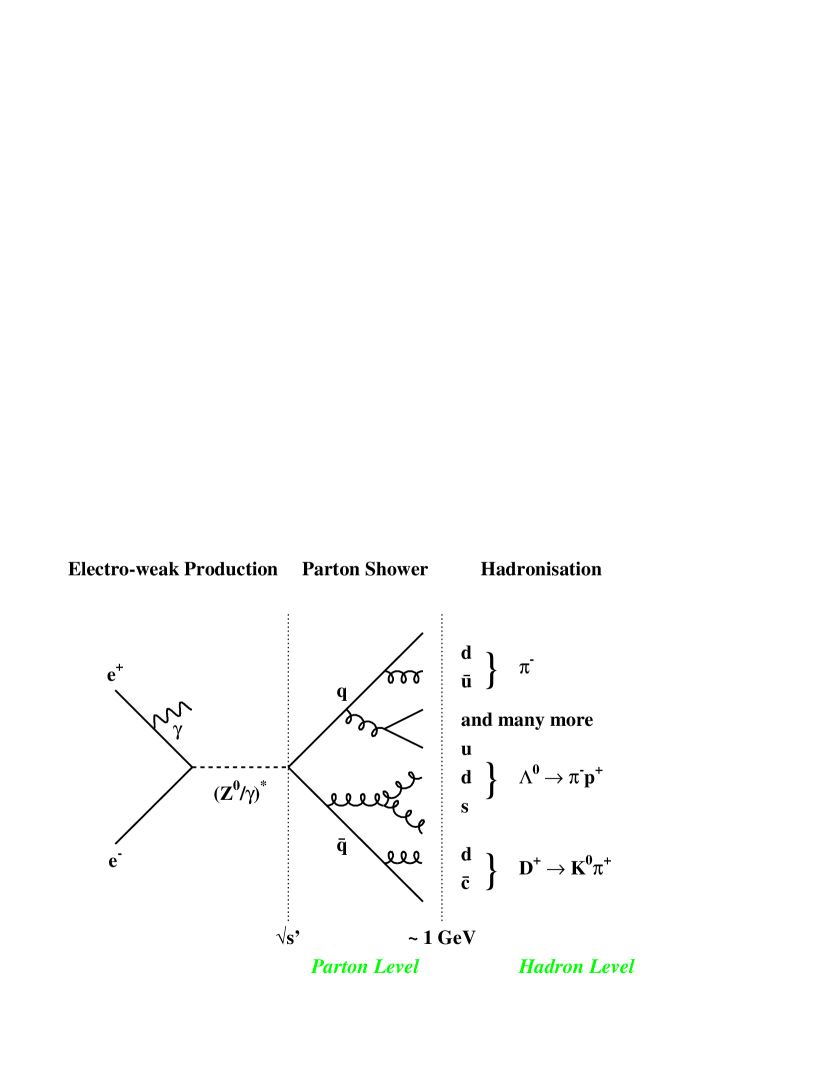
Figure 1: Schematic view of hadron production in $\mathrm{e^{+}e^{-}}$ annihilation.

The current understanding of hadron production in $\mathrm{e^{+}e^{-}}$ annihilation in the Standard Model is shown schematically in figure 1. The colliding electron and positron annihilate into a photon or $\mathrm{Z^{0}}$, possibly with additional radiation of energetic photons from the incoming beam particles (initial state radiation or ISR). The intermediate photon is always virtual with its invariant mass equal to the invariant mass $\sqrt{s^{\prime}}$ of the $\mathrm{e^{+}e^{-}}$ system at collision after ISR while the $\mathrm{Z^{0}}$ can be produced on mass-shell when $\sqrt{s^{\prime}}\simeq M_{\mathrm{Z^{0}}}$. The intermediate photon or $\mathrm{Z^{0}}$ then decays into a $\mathrm{q\overline{q}}$ state which can in turn radiate gluons. The continuing processes of gluon radiation and $\mathrm{q\overline{q}}$ production result in a parton shower which only terminates when the partons (quarks and gluons) reach energy scales of $\sim 1$ GeV. Final states at this stage are referred to as parton-level. At these scales the increasing strong coupling causes the formation of colourless bound states of quarks, i.e. hadrons. This process, known as hadronisation, is not well understood at a fundamental level in QCD but many successful models based on QCD have been developed. The hadronic final state after decays of short lived particles (usually defined to have lifetimes $<300$ ps) is said as being at the hadron-level.

It is well known that the hadronic final states in $\mathrm{e^{+}e^{-}}$ annihilation show a so-called jet structure, i.e. several groups of particles are observed in relatively small and separate regions of the solid angle around the interaction point. These structures are interpreted as remnants of the $\mathrm{q\overline{q}}$ pair from the virtual photon or $\mathrm{Z^{0}}$ decay and possible energetic gluon radiation. Many definitions of jet finding algorithms [1, 2] or event shape observables (see e.g.  [3, 4]) are used to quantify the jet structure and compare with predictions from QCD.

Jet finding algorithms cluster particles lying closely together in phase space. As an example in the Durham algorithm [5] the distance between two particles $i$ and $j$ with energies $E_{i}$ and $E_{j}$ and spanning the angle $\theta_{ij}$ is defined as $y_{ij}=2E_{i}E_{j}(1-\cos\theta_{ij})/s$. The pair of particles with the smallest $y_{ij}$ is combined into a pseudo-particle by adding the four-momenta and is then discarded. The procedure is iterated until only one jet remains. One can now study the jet structure as a function of the resolution parameter $y_{\mathrm{cut}}$ and e.g. determine the fraction of 3-jet events at a fixed value of $y_{\mathrm{cut}}$. Alternatively, the value of $y_{ij}=y_{32}$ where an event changes from a 3-jet to a 2-jet configuration is characteristic for its structure, i.e. a large value of $y_{32}$ indicates the presence of a significant third jet.

At the time of writing data of observables such as jet production rates or event shape distributions measured at centre-of-mass energies $\sqrt{s}$ ranging from 14 to 209 GeV are available. These are especially interesting, because many QCD predictions are strongly energy dependent due to the running of the strong coupling $\alpha_{\mathrm{S}}(Q)$. In leading order the running of $\alpha_{\mathrm{S}}$ is expressed as

$$\alpha_{\mathrm{S}}(Q)=\alpha_{\mathrm{S}}(\mu)/(1+2\beta_{0}\alpha_{\mathrm{S}}(\mu)\ln(\mu/Q))$$ (1)

with $\beta_{0}=(11C_{A}-2n_{f})/(12\pi)$. The value $\alpha_{\mathrm{S}}(Q)$ at a scale $Q$ is given by $\alpha_{\mathrm{S}}(\mu)$ at a reference scale $\mu$ and the logarithmic ratio of the energy scales $2\ln(Q/\mu)$. However, hadronisation effects scale like $1/Q^{n}$, with $n=1$ for many jet algorithms or event shape observables, implying that a meaningful comparison of QCD predictions with data requires a detailed understanding of the scale dependencies of perturbative QCD and as well as of the hadronisation effects. The present $\mathrm{e^{+}e^{-}}$ data allow to study these problems in a controlled way.

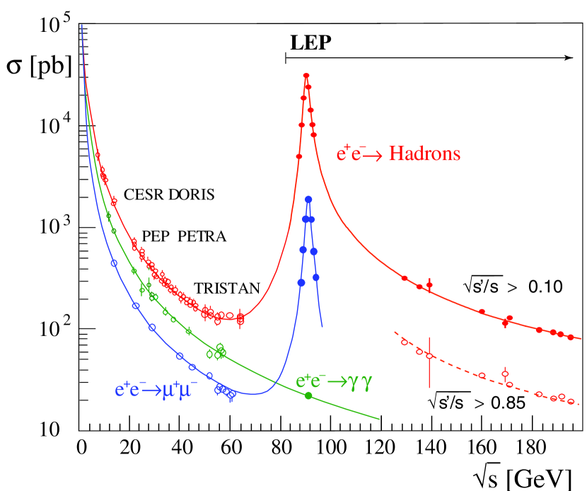
Figure 2: Cross sections for various $\mathrm{e^{+}e^{-}}$ annihilation processes as indicated on the figure [6].

The selection of $\mathrm{e^{+}e^{-}}$ annihilation into hadronic final states has to consider different experimental conditions at the various cms energies. Figure 2 shows the total cross sections for hadron production, $\mu^{+}\mu^{-}$ pair production and two-photon interactions [6]. At $\sqrt{s}<M_{\mathrm{Z^{0}}}$ backgrounds stem from two-photon processes, $\tau^{+}\tau^{-}$ pair production and events with hard ISR. For example in the JADE data recorded between $\sqrt{s}=14$ and 44 GeV after demanding large total energy, balance of momentum along the beam axis and large particle multiplicity the total background is reduced to about 1% with a selection efficiency of about 60% [7]. On the $\mathrm{Z^{0}}$ peak similar event selections reduce the background to less than 1% with almost 100% selection efficiency. Above the $\mathrm{Z^{0}}$ peak for $\sqrt{s}>2M_{\mathrm{W}}$ backgrounds from hadron production mainly via production of $\mathrm{W^{+}W^{-}}$ pairs decaying both hadronically become important. The prominent 4-jet structure of the $\mathrm{W^{+}W^{-}}$ events and their different kinematic properties compared to $\mathrm{e^{+}e^{-}}\rightarrow\mathrm{q\overline{q}}$ events allows to reduce backgrounds to less than 10% at selection efficiencies of about 80%.

2 HARD QCD

2.1 Measurements of $\alpha_{\mathrm{S}}$

The strong coupling is in QCD predictions for massless partons the only free parameter. A fit of the theoretical prediction to the data with $\alpha_{\mathrm{S}}$ as a free parameter yields a measurement of $\alpha_{\mathrm{S}}(Q)$ where $Q$ is identified with the hard scale of the process, i.e. $Q=\sqrt{s}$. Hadronisation effects are not part of the perturbative QCD prediction and are usually treated as a correction which is applied to the theory before comparison with the data. The choice between several hadronisation models implemented in Monte Carlo generator programs and uncertainties in the experimentally adjusted free parameters of the models are reflected in the systematic uncertainties of the $\alpha_{\mathrm{S}}$ determinations.

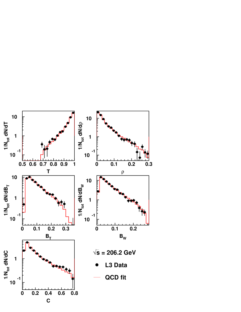
Figure 3: Data from L3 of event shape observables measured at $\sqrt{s}=206.2$ GeV. Superimposed are $\mathcal{O}(\alpha_{\mathrm{S}}^{2})$+NLLA QCD fits [8].

Figure 3 shows the measurement of $\alpha_{\mathrm{S}}(206.2~{}\mathrm{GeV})$ by L3 [8] using a set of five event shape observables Thrust $T$, Heavy Jet Mass $\rho$, Total and Wide Jet Broadening $B_{T}$ and $B_{W}$, and C-parameter $C$. For these observables matched $\mathcal{O}(\alpha_{\mathrm{S}}^{2})$+NLLA QCD calculations [9, 10, 11] are available, which provide reliable predictions over a large part of the phase space populated by 2- and 3-jet events. The combined result of the five measurements is $\alpha_{\mathrm{S}}(206.2~{}\mathrm{GeV})=0.113\pm 0.002\mathrm{(stat.)}\pm 0.005\mathrm{(syst.)}$.

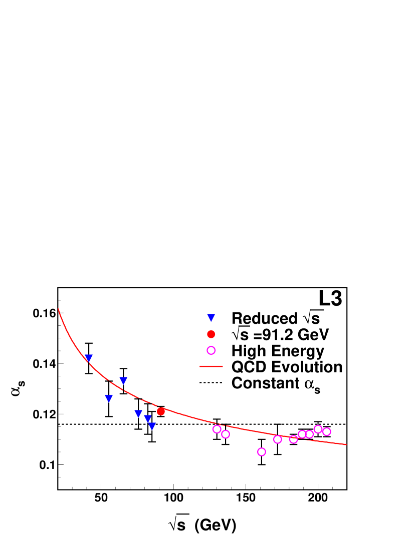
Figure 4: Results of $\alpha_{\mathrm{S}}(\sqrt{s})$ from L3 compared with the expectation from QCD for the running of $\alpha_{\mathrm{S}}$ (solid line) and with $\alpha_{\mathrm{S}}=\mathrm{const.}$ (dashed line) [8].

Figure 4 presents the results of similar analysis performed by L3 at the other LEP 2 energy points, at LEP 1 on the $\mathrm{Z^{0}}$ peak and using hadronic $\mathrm{Z^{0}}$ decays with hard final state photon radiation (FSR) for measurements at $\sqrt{s}<M_{\mathrm{Z^{0}}}$. The error bars show the experimental and statistical uncertainties only. The solid line shows a fit of the QCD prediction for the running of $\alpha_{\mathrm{S}}$ with the result $\alpha_{\mathrm{S}}(M_{\mathrm{Z^{0}}})=0.123\pm 0.001\exp\pm 0.006\mathrm{(theo.)}$ and $\chi^{2}/\mathrm{d.o.f.}=18/15$. The assumption of $\alpha_{\mathrm{S}}$=const. results in $\chi^{2}/\mathrm{d.o.f.}=52/15$; the data thus support the running of $\alpha_{\mathrm{S}}$ as predicted by QCD. Similar analyses by the LEP collaborations are [12, 13].

The data of the former JADE experiment taken between 1979 and 1986 at PETRA/DESY at $\sqrt{s}=14$ to 44 GeV have been re-analysed recently [7]. The analysis employs modern Monte Carlo event generators together with the original detector simulation program to obtain more reliable experimental corrections with reduced statistical and systematic uncertainties. The contribution of $\mathrm{e^{+}e^{-}}\rightarrow\mathrm{b\overline{b}}$ events is subtracted to reduce the effects of heavy quark masses and heavy hadron decays on the analysis. The data can be compared directly with QCD predictions for massless partons corrected for hadronisation effects. Several event shape observables are used to determine $\alpha_{\mathrm{S}}$ in the same way as the LEP collaborations using the best currently available matched $\mathcal{O}(\alpha_{\mathrm{S}}^{2})$+NLLA QCD calculations.

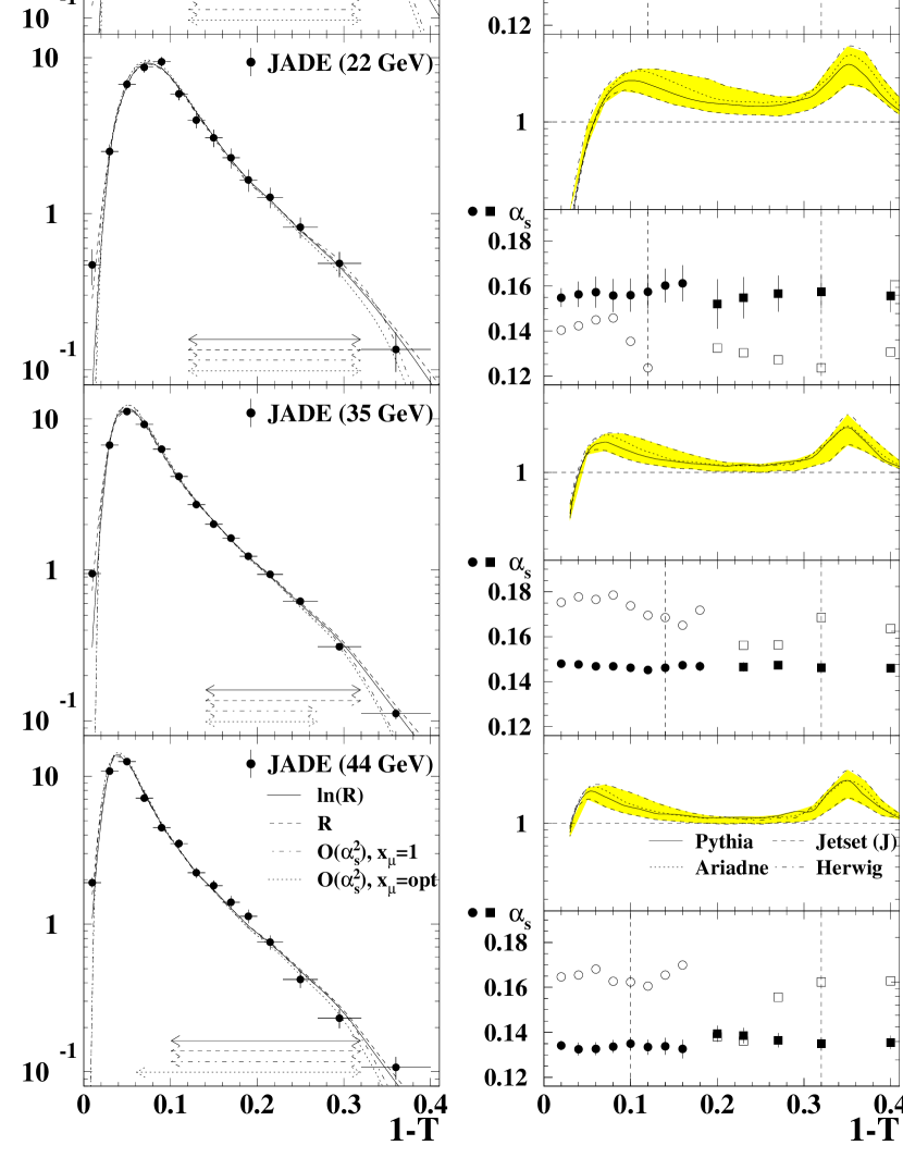
Figure 5: Data for $1-T$ from JADE at $\sqrt{s}=14$, 22, 35 and 44 GeV are shown on the left with $\mathcal{O}(\alpha_{\mathrm{S}}^{2})$+NLLA or $\mathcal{O}(\alpha_{\mathrm{S}}^{2})$ QCD fits superimposed (lines). On the right the hadronisation corrections $K_{i}$ are shown with uncertainties as grey bands [7].

The results of fits to $1-T$ are shown in figure 5. The diagrams show the data for $1-T$ at $\sqrt{s}=14$, 22, 35 and 44 GeV corrected for experimental effects. A decrease of the shoulder at large $1-T$ with increasing $\sqrt{s}$ is clearly visible; this observation corresponds to the expected lower fraction of events with hard gluon radiation due to the running of $\alpha_{\mathrm{S}}$. Superimposed are the results of QCD fits using matched $\mathcal{O}(\alpha_{\mathrm{S}}^{2})$+NLLA ($\ln(\mathrm{R})$- and R-matching) or $\mathcal{O}(\alpha_{\mathrm{S}}^{2})$ calculations corrected for hadronisation effects, which generally describe the data well. The hadronisation corrections $K_{i}$ with uncertainties are shown as grey bands. The hadronisation corrections are large with large uncertainties at low $\sqrt{s}$ but become much smaller with increasing $\sqrt{s}$. The results for $\alpha_{\mathrm{S}}(\sqrt{s})$ are $\alpha_{\mathrm{S}}(14~{}\mathrm{GeV})=0.170\pm 0.019$, $\alpha_{\mathrm{S}}(22~{}\mathrm{GeV})=0.151\pm 0.013$, $\alpha_{\mathrm{S}}(35~{}\mathrm{GeV})=0.146\pm 0.012$ and $\alpha_{\mathrm{S}}(44~{}\mathrm{GeV})=0.131\pm 0.009$. The data together with other compareable results from the LEP experiments and SLD are in good agreement within the experimental errors with the QCD prediction for the running $\alpha_{\mathrm{S}}$ based on $\alpha_{\mathrm{S}}(M_{\mathrm{Z^{0}}})=0.118\pm 0.003$ [14]. As above a fit assuming $\alpha_{\mathrm{S}}$=const. results in a $\chi^{2}$ probability of $\sim 10^{-5}$.

A novel method to determine the strong coupling $\alpha_{\mathrm{S}}$ uses the rate of 4-jet events $\mathrm{R}_{4}$ determined using the Durham algorithm [15, 16]. Recently the NLO corrections for observables sensitive to at least four partons in the final state, i.e. corrections of $\mathcal{O}(\alpha_{\mathrm{S}}^{3})$, became available [17, 18]. These calculations are matched with existing NLLA calculations.

A measurement of $\alpha_{\mathrm{S}}(M_{\mathrm{Z^{0}}})$ based on these predictions is presented in figure 6 [15]. The uncorrected data for $\mathrm{R}_{4}$ measured using $2.5\cdot 10^{6}$ hadronic $\mathrm{Z^{0}}$ decays using the Durham algorithm are shown as a function of the jet resolution parameter $y_{\mathrm{cut}}$. The line shows the fit of the $\mathcal{O}(\alpha_{\mathrm{S}}^{3})$+NLLA (R-matching) theory corrected for hadronisation and detector effects. The fit is performed using only the bins within the fit range as indicated where the total correction factors deviate from unity by less than 10%. The result of the fit for fixed renormalisation scale parameter $x_{\mu}=1$ is $\alpha_{\mathrm{S}}(M_{\mathrm{Z^{0}}})=0.1170\pm 0.0022$ using the conservatively estimated total error from [15]. The fit is seen to describe the precise data fairly well. The similar analysis of [16] uses only the $\mathcal{O}(\alpha_{\mathrm{S}}^{3})$ calculations with experimentally optimised renormalisation scale and finds $\alpha_{\mathrm{S}}(M_{\mathrm{Z^{0}}})=0.1178\pm 0.0029$ with $x_{\mu}^{2}=0.015$. These measurements have comparatively small uncertainties and belong to the group of the most precise determinations of $\alpha_{\mathrm{S}}$.

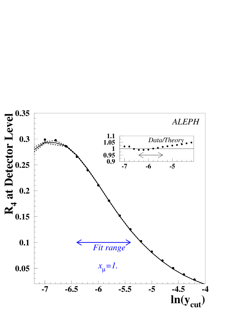
Figure 6: The 4-jet fraction $\mathrm{R}_{4}$ determined using the Durham algorithm is shown as a function of $y_{\mathrm{cut}}$ without corrections. Superimposed is a fit of $\mathcal{O}(\alpha_{\mathrm{S}}^{3})$+NLLA QCD (solid line) [15].

2.2 Running b quark mass

The QCD predictions discussed so far have been made for massless partons. The effects of massive quarks on the perturbative QCD predictions are known in $\mathcal{O}(\alpha_{\mathrm{S}}^{2})$ as well [19, 20, 21]. The mass of the heavy quark $m_{\mathrm{b}}$ identified with the b quark at LEP energies becomes an additional parameter of the theory and is subject to renormalisation analogously to the strong coupling constant. As a result the heavy quark mass $m_{\mathrm{b}}$ will depend on the scale of the hard process in which the heavy quark participates. In leading order in the $\overline{\mathrm{MS}}$ renormalisation scheme the running b-quark mass is $m_{\mathrm{b}}(Q)=M_{\mathrm{b}}(\alpha_{\mathrm{S}}(Q)/\pi)^{12/23}$, where $M_{\mathrm{b}}$ is the so-called pole mass defined by the pole of the renormalised heavy quark propagator. The running $m_{\mathrm{b}}$ is known to four-loop accuracy [22]. Using low energy measurements of $m_{\mathrm{b}}(m_{\mathrm{b}})$ one finds that $m_{\mathrm{b}}(M_{\mathrm{Z^{0}}})\simeq 3$ GeV.

The mass of the b quark $m_{\mathrm{b}}$ is experimentally accessible in hadronic $\mathrm{Z^{0}}$ decays, because i) about 21% of the decays are $\mathrm{Z^{0}}\rightarrow\mathrm{b\overline{b}}$ and these events can be identified with high efficiency and purity, ii) event samples of $\mathcal{O}(10^{6})$ events are available and iii) observables like the 3-jet rate $\mathrm{R}_{3}(y_{\mathrm{cut}})$ in the JADE or Durham algorithm can have enhanced mass effects going like $m_{\mathrm{b}}^{2}/M_{\mathrm{Z^{0}}}^{2}/y_{\mathrm{cut}}$ [23]. In the experimental analyses [24, 25, 26, 27, 28] the ratio $\mathrm{B}_{3}=\mathrm{R^{b}}_{3}/\mathrm{R^{l}}_{3}$, $\mathrm{R^{b}}_{3}$($\mathrm{R^{l}}_{3}$) are the 3-jet rates in b quark (light quark) events, is studied which reduces the influence of common systematics.

Figure 7: The figures show distributions of $\mathrm{B}_{3}$ determined using the Durham or JADE E0 jet finding algorithms before and after all corrections. The solid lines in the lower row of figures give the uncertainties on $\mathrm{B}_{3}$. The vertical dashed lines indicate the values of $y_{\mathrm{cut}}$ where the QCD predictions are calculated [25].

Figure 7 shows $\mathrm{B}_{3}(y_{\mathrm{cut}})$ measured by OPAL [25] before and after detector and hadronisation corrections for the JADE E0 and the Durham algorithm. One observes that the effect of the b quark mass is about 5% on $\mathrm{B}_{3}$ with reasonable uncertainties as indicated by the bands. The effect goes in opposite directions for JADE E0 and the Durham algorithm, because in the JADE type algorithms based on invariant mass to cluster jets the large b quark mass causes an enhancement of $\mathrm{B}_{3}$ while in the Durham algorithm the reduced phase space for hard gluon emmission dominates thus reducing $\mathrm{B}_{3}$ [26].

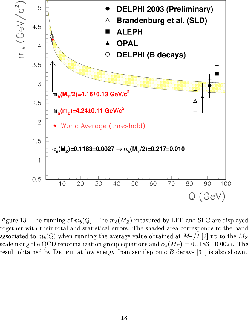
Figure 8: Measurements of $m_{\mathrm{b}}(Q)$ at low and high energies $Q$ are compared with the QCD expectation for the running of $m_{\mathrm{b}}(Q)$ [28].

Figure 8 gives an overview over presently available measurements of $m_{\mathrm{b}}(M_{\mathrm{Z^{0}}})$ [28]. These are compared with low energy measurements and the QCD prediction for the running of $m_{\mathrm{b}}(Q)$. The predicted range of $m_{\mathrm{b}}(M_{\mathrm{Z^{0}}})$ is in good agreement with the measurements. The measurements of $m_{\mathrm{b}}(M_{\mathrm{Z^{0}}})$ of [25, 26, 27, 28] can be averaged assuming the statistical errors to be uncorrelated, the experimental and hadronisation uncertainties to be partially correlated and the theory uncertainties to be fully correlated. The result is $m_{\mathrm{b}}(M_{\mathrm{Z^{0}}})=(2.92\pm 0.03\mathrm{(stat.)}\pm 0.31\mathrm{(syst.)})$ GeV, which may be compared with the average of low energy measurements $m_{\mathrm{b}}(m_{\mathrm{b}})=(4.24\pm 0.11)$ GeV [29]. The difference becomes $m_{\mathrm{b}}(M_{\mathrm{Z^{0}}})-m_{\mathrm{b}}(m_{\mathrm{b}})=(1.32\pm 0.33)$ GeV which is non-zero by four standard deviations thus providing strong experimental evidence for the running heavy quark mass in QCD.

3 QCD GAUGE STRUCTURE

QCD as the gauge theory of strong interactions assumes that quarks carry one out of three strong charges, referred to as colour. The requirement of local gauge symmetry under SU(3) transformations in the colour space generates the gauge bosons of QCD: an oktett of gluons each carrying colour charge and anti-charge, see e.g. [30]. The gluons can thus interact with themselves; it is due to this property of the QCD gauge bosons that the theory explains confinement and asymptotic freedom via the running of the strong coupling $\alpha_{\mathrm{S}}$.

In perturbative QCD at NLO three fundamental vertices contribute: i) the quark-gluon vertex with colour factor $C_{A}$, ii) the gluon-gluon vertex with colour factor $C_{A}$ and iii) the $\mathrm{q\overline{q}}$ production from a gluon with colour factor $T_{F}n_{f}$, see e.g. [31]. The colour factors are $C_{F}=4/3$, $C_{A}=3$ and $T_{F}n_{f}=1/2\cdot 5$ in QCD with SU(3) gauge symmetry and specify the relative contribution of the corresponding vertex to observables. In NLO QCD the prediction for an observable $R$ is $R=A\alpha_{\mathrm{S}}+(B_{C_{F}}C_{F}+B_{C_{A}}C_{A}+B_{T_{F}}T_{F}n_{f})C_{F}\alpha_{\mathrm{S}}^{2}$; NLLA predictions e.g. for event shapes or jet rates decompose in a similar way. For NLO predictions for 4-jet observables an analogous decomposition in terms of the six possible products of two out of the three colour factors holds [32].

Experimental investigations of the gauge structure of QCD are possible because of the different angular momenta in the initial and final states of the fundamental vertices. It is an important test of QCD to probe the gauge structure in experiments. Several techniques with rather different experimental and theoretical uncertainties have been developed; we will discuss here some recent results.

3.1 Four-jet events

The LEP experiments ALEPH [15] and OPAL [33] have analysed 4-jet final states from hadronic $\mathrm{Z^{0}}$ decays using the recent QCD NLO predictions (see e.g. [32] and references therein). The 4-jet final states are selected by clustering events using the Durham algorithm [5] with $y_{\mathrm{cut}}=0.008$ and demanding four jets. At this value of $y_{\mathrm{cut}}$ the 4-jet fraction is relatively large ($\mathrm{R}_{4}\simeq 7$%) and the four jets are well separated.

The energy-ordered 4-momenta $p_{i},i=1,\ldots,4$ of the jets are used to calculate the angular correlation observables (see  [15, 33] for details). As an example, the Bengtsson-Zerwas angle $\chi_{\mathrm{BZ}}$ is defined by $\chi_{\mathrm{BZ}}=\angle([\vec{p_{1}}\times\vec{p_{2}}],[\vec{p_{3}}\times\vec{p_{4}}])$, i.e. the angle between the two planes spanned by the momentum vector pairs $(\vec{p_{1}},\vec{p_{2}})$ and $(\vec{p_{3}},\vec{p_{4}})$. Assuming that energy ordering selected the primary quarks from the $\mathrm{Z^{0}}$ decay as $(p_{1},p_{2})$ the observable $\chi_{\mathrm{BZ}}$ is sensitive to the decay of an intermediate gluon to gluons (vertex ii)) or quarks (vertex iii)) and the competing process of radiation of a second gluon from a primary quark (vertex i)).

Figure 9: The distribution of $|\cos\chi_{\mathrm{BZ}}|$ before corrections is shown (solid points). Superimposed is a fit of NLO QCD (solid lines) [15].

Figure 9 presents the uncorrected distribution of $\cos(\chi_{\mathrm{BZ}})$ measured by ALEPH [15]. Superimposed on the data points is the result of a simultaneous fit of the NLO QCD predictions to four angular correlations including $\chi_{\mathrm{BZ}}$ and the distribution of $\mathrm{R}_{4}$. From the fit values for $\alpha_{\mathrm{S}}(M_{\mathrm{Z^{0}}})$ and the colour factors $C_{A}$ and $C_{F}$ are extracted. The results from ALEPH are $\alpha_{\mathrm{S}}(M_{\mathrm{Z^{0}}})=0.119\pm 0.027$, $C_{A}=2.93\pm 0.60$ and $C_{F}=1.35\pm 0.27$; from OPAL we have $\alpha_{\mathrm{S}}(M_{\mathrm{Z^{0}}})=0.120\pm 0.023$, $C_{A}=3.02\pm 0.55$ and $C_{F}=1.34\pm 0.26$. The systematic errors are dominated by uncertainties from the hadronisation corrections and theoretical errors from estimating missing higher order contributions.

3.2 Event shape fits

In this analysis [34] the decomposition of the $\mathcal{O}(\alpha_{\mathrm{S}}^{2})$+NLLA QCD predictions for event shape observables into terms proportional to the colour factors is used. Since the sensitivity of event shape distributions measured at LEP 1 alone is not sufficient [35] data from $\sqrt{s}=14$ to 189 GeV are used. In this way the colour structure of the running of the strong coupling contributes as well. Hadronisation corrections are implemented using analytic predictions known as power corrections (see [34] and references therein). The power corrections essentially predict that hadronisation effects cause a shift of the perturbative distribution proportial to $1/\sqrt{s}$ in the region where the $\mathcal{O}(\alpha_{\mathrm{S}}^{2})$+NLLA predictions are reliable. The advantage of using power corrections instead of Monte Carlo model based hadronisation corrections is that the colour structure of the power corrections is known and can be varied in the fit.

In the analysis simultaneous fits of $\alpha_{\mathrm{S}}(M_{\mathrm{Z^{0}}})$, $C_{A}$ and $C_{F}$ to data for the event shape observables $1-T$ at $\sqrt{s}=14$ to 189 GeV and $C$ at $\sqrt{s}=35$ to 189 GeV are performed. The data for $1-T$ and $C$ are analysed separatly and the results are combined. The results are $\alpha_{\mathrm{S}}(M_{\mathrm{Z^{0}}})=0.119\pm 0.010$, $C_{A}=2.84\pm 0.24$ and $C_{F}=1.29\pm 0.18$ and are shown on figure 12 below. The errors are dominated by uncertainties from the hadronisation correction and from experimental effects.

3.3 Scaling violation in gluon and quark jets

Jets originating from quarks or gluons should have different properties due to the different colour charge carried by quarks or gluons [36, 37]. In an analysis by DELPHI [38] the scaling violation of the fragmentation function (FF) in gluon and quark jets at different energies is compared. From a sample of $3.7\cdot 10^{6}$ hadronic $\mathrm{Z^{0}}$ decays planar 3-jet events with well reconstructed jets are selected using the Durham or Cambridge algorithms, but without imposing a fixed value of $y_{\mathrm{cut}}$ in order to reduce biases [39]. In events with the two angles between the most energetic jet and the other jets in the range between 100^o and 170^o a b-tagging procedure is applied to the jets. Gluon jets are identified indirectly as the jets without a successful b-tag. Jets originating from light (udsc) quarks are taken from events which failed the b-tagging. A correction procedure based on efficiencies and purities determined by Monte Carlo simulation yields results for pure gluon or quark jets.

The jet energy scale is calculated according to $\kappa_{\mathrm{H}}=E_{\mathrm{jet}}\sin(\theta/2)$, where $\theta$ is the angle w.r.t. to the closest jet. This definition takes colour coherence effects into account [40]. The FF in a jet $D^{H}(x_{\mathrm{E}},\kappa_{\mathrm{H}})$ is given by the distribution of $x_{\mathrm{E}}=E_{\mathrm{hadron}}/\kappa_{\mathrm{H}}$ for the hadrons assigned to the jet. The evolution of the FFs of gluon and quark jets with jet energy scale $\kappa_{\mathrm{H}}$ is studied in intervals of $x_{\mathrm{E}}$. Figure 10 presents the quantity $\mathrm{d}D^{H}(x_{\mathrm{E}},\kappa_{\mathrm{H}})/\mathrm{d}\log(\kappa_{\mathrm{H}})$, i.e. the slopes of the scaling violation for a given interval of $x_{\mathrm{E}}$, for quark and gluon jets. The steeper slopes corresponding to stronger scaling violations of gluon compared to quark jets is clearly visible. A fit of the scaling violations based on the LO QCD prediction (DGLAP equation) allows to extract the ratio $C_{A}/C_{F}$ resulting in $C_{A}/C_{F}=2.26\pm 0.16$.

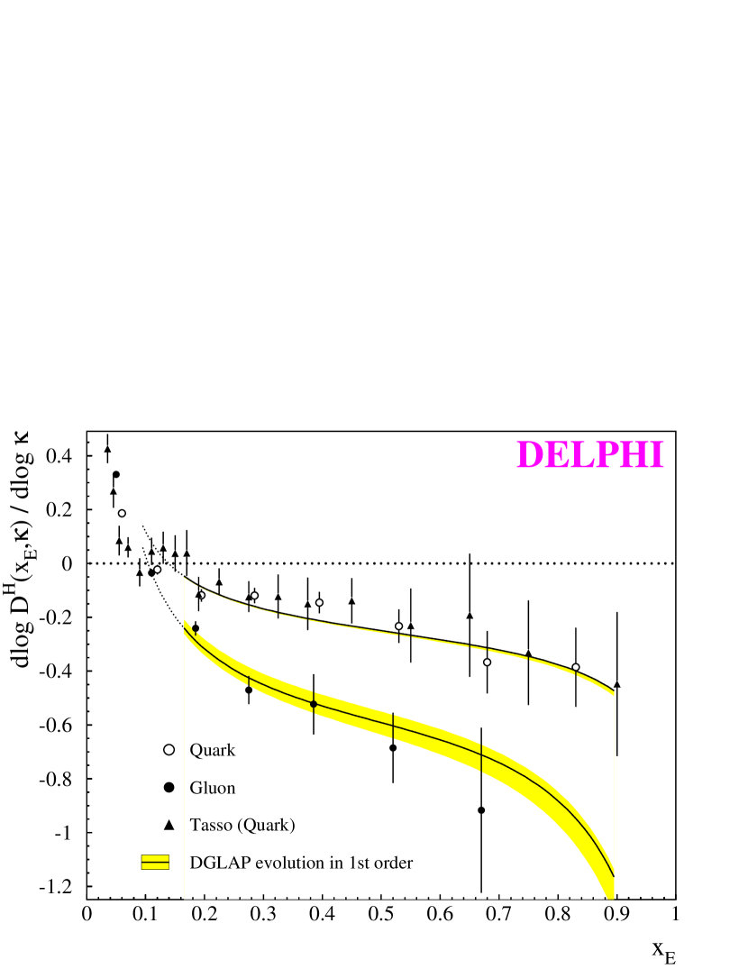
Figure 10: Measurements of $\mathrm{d}D^{H}(x_{\mathrm{E}},\kappa_{\mathrm{H}})/\mathrm{d}\log(\kappa_{\mathrm{H}})$ are shown for gluon (solid points) and quark jets (open circles and solid triangles). The lines represent a fit of the LO QCD prediction [38].

3.4 Multiplicity in unbiased gluon jets

In this analysis [41] the evolution with energy scale of the charged particle multiplicities $N^{\mathrm{ch.}}_{\mathrm{gg}}$ and $N^{\mathrm{ch.}}_{\mathrm{q\overline{q}}}$ for gluon and quark jets is used to measure the colour charge ratio $C_{A}/C_{F}$. The inclusive multiplicity $N^{\mathrm{ch.}}_{\mathrm{incl.}}$ is measured in hadronic $\mathrm{Z^{0}}$ decays as a function of the 3-jet transverse momentum scale $k_{\perp,\mathrm{Lu}}=\ln(s_{\mathrm{qg}}s_{\mathrm{\overline{q}g}}/(s\Lambda_{\mathrm{QCD}})$ where $s_{\mathrm{qg}}$ and $s_{\mathrm{\overline{q}g}}$ are the invariant masses between the gluon and the quark jets [39, 42]. The analysis reconstructs three jets in all events by adjusting the value of $y_{\mathrm{cut}}$ in the Durham algorithm, selects one-fold symmetric Y-events [43] and identifies the lowest energy jet as the gluon jet. By comparing with measurements of $N^{\mathrm{ch.}}_{\mathrm{q\overline{q}}}(k_{\perp,\mathrm{Lu}})$ the multiplicity in unbiased gluon jets $N^{\mathrm{ch.}}_{\mathrm{gg}}$ can be extracted as a function of the jet energy scale $k_{\perp,\mathrm{Lu}}$: $N^{\mathrm{ch.}}_{\mathrm{gg}}(k_{\perp,\mathrm{Lu}})=2(N^{\mathrm{ch.}}_{\mathrm{incl.}}(k_{\perp,\mathrm{Lu}})-N^{\mathrm{ch.}}_{\mathrm{q\overline{q}}}(k_{\perp,\mathrm{Lu}}))$.

Figure 11 shows the data for $N^{\mathrm{ch.}}_{\mathrm{gg}}$ together with compareable data at lower and higher jet energy scales $k_{\perp,\mathrm{Lu}}$ from CLEO and OPAL. The solid line represents the result of a fit of the QCD prediction for the evolution of $N^{\mathrm{ch.}}_{\mathrm{gg}}$ compared to $N^{\mathrm{ch.}}_{\mathrm{q\overline{q}}}$ [39]. The fit with $C_{A}/C_{F}$ as a free parameter yields $C_{A}/C_{F}=2.23\pm 0.14$. This analysis is complementary to the analysis of scaling violations discussed above because the multiplicity is dominated by low energy particles while the scaling violation is dominated by high energy particles with large $x_{\mathrm{E}}$.

Figure 11: Measurements of $N^{\mathrm{ch.}}_{\mathrm{gg}}(Q)$ are shown using 3-jet events (solid points) and other data (solid triangles). Superimposed are predictions of Monte Carlo generators (dashed and dash-dotted lines) and of the QCD fit (solid line) [41].

3.5 Colour factor averages

The measurements of the colour factors $C_{A}$ and $C_{F}$ or of $C_{A}/C_{F}=x$ discussed above can be combined into average values of $C_{A}$ and $C_{F}$ taking into account correlations between $C_{A}$ and $C_{F}$ as well as between different experiments. The variables $x$ and $y=T_{F}/C_{F}$ are used to define the $\chi^{2}$ function

$$\chi^{2} = \sum_{i}(x_{i}-\bar{x})v^{(xy)}_{i}(y_{i}-\bar{y})+$$

$$\sum_{ij}(x_{i}-\bar{x})v^{(x)}_{ij}(x_{j}-\bar{x})+$$

$$\sum_{ij}(y_{i}-\bar{y})v^{(y)}_{ij}(y_{j}-\bar{y})\;\;,$$

where $\bar{x}$ and $\bar{y}$ are the averages, the indices $i,j$ count experiments, $v^{(xy)}_{i}$, $v^{(x)}_{ij}$ and $v^{(y)}_{ij}$ are elements of the inverses of the corresponding covariance matrices for the $x_{i}$ and $y_{i}$ within experiment $i$ and for the $x_{i}$ and $y_{i}$ between experiments. The averages $\bar{x}$ and $\bar{y}$ are converted to the average values $\overline{C}_{A}$ and $\overline{C}_{F}$ after the fit is performed.

The input data for $x$ and $y$ are directly taken from [15, 33, 38, 41] while the results from [34] have to be converted.

The covariance matrices between experiments are constructed as follows: ALEPH and OPAL 4-jet analyses experimental and hadronisation errors partially and theory errors fully correlated, 4-jet analyses and event shape analysis hadronisation errors partially and theory errors fully correlated, and 4-jet and event shape analyses and DELPHI FF and OPAL $N^{\mathrm{ch.}}_{\mathrm{gg}}$ analyses theory errors partially correlated.

The averaging fit is done using only the first term of equation 3.5 to determine the averages $\overline{C}_{A}$ and $\overline{C}_{F}$, using only statistical correlations in the first term to determine the statistical errors and using the full covariance matrix to determine the total errors. The final results are $\overline{C}_{A}=2.89\pm 0.03\mathrm{(stat.)}\pm 0.21\mathrm{(syst.)}$, $\overline{C}_{F}=1.30\pm 0.01\mathrm{(stat.)}\pm 0.09\mathrm{(syst.)}$ with correlation coefficient $\rho=0.82$. The relative total uncertainties are about 8% for both $\overline{C}_{A}$ and $\overline{C}_{F}$.

Figure 12 presents the results of the individual analysis in a $C_{F}$ vs. $C_{A}$ plane together with the combined result and the expectations of QCD based on the SU(3) gauge symmetry and various other gauge symmetries. The correlation coefficients for [15, 33] were calculated from the references. The error ellipses refer to 86% CL. The combined result is in good agreement with the individual analyses and with standard SU(3) QCD while the total uncertainties are substantially reduced. The other possibilities for gauge symmetries shown on the figure are clearly ruled out.

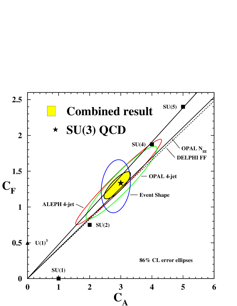
Figure 12: The figure presents various measurements of the colour factors $C_{A}$ and $C_{F}$ discussed in this report. The ellipses show the correlated measurements using 4-jet events [15, 33] or event shape distributions [34] while the lines represent the results of determinations of $C_{A}/C_{F}$ from DELPHI [38] (dashed) and OPAL [41] (solid). The upper solid and dashed lines overlap. The grey filled ellipsis displays the combined result for $\overline{C}_{A}$ and $\overline{C}_{F}$ (see text). The solid triangle and squares show the expectations for various assumptions for the gauge symmetry of QCD as indicated on the figure.

4 CONCLUSIONS

Jet physics in $\mathrm{e^{+}e^{-}}$ annihilation based on data from $\sqrt{s}=14$ to 207 GeV allows to study many aspects of QCD. Precision measurements of the strong coupling $\alpha_{\mathrm{S}}$ at many points of $\sqrt{s}$ gave convincing evidence for the running of the strong coupling as predicted by the theory.

A combination of measurements of the mass of the b-quark $m_{\mathrm{b}}(M_{\mathrm{Z^{0}}})$ at the $M_{\mathrm{Z^{0}}}$ energy scale using jet production rates was performed. The resulting value

$$m_{\mathrm{b}}(M_{\mathrm{Z^{0}}})=(2.92\pm 0.03\mathrm{(stat.)}\pm 0.31\mathrm{(syst.)})\mathrm{GeV}$$ (3)

compared with low energy measurements resulted in strong evidence for the running of the b-quark mass analogously to the running of $\alpha_{\mathrm{S}}$.

The investigation of the gauge structure of QCD was discussed for several different methods: angular correlations in 4-jet final states from hadronic $\mathrm{Z^{0}}$ decays, global fits of event shape data at many points of $\sqrt{s}$, the scaling violation of the FF of gluon and quark jets and the evolution with energy scale of the charged particle multiplicity $N^{\mathrm{ch.}}_{\mathrm{gg}}$ determined from 3-jet events. The results of the analyses were combined taking correlations between the colour factor measurements into account with the results:

$$\overline{C}_{A} = 2.89\pm 0.03\mathrm{(stat.)}\pm 0.21\mathrm{(syst.)}\;\;,$$ (4)

$$\overline{C}_{F} = 1.30\pm 0.01\mathrm{(stat.)}\pm 0.09\mathrm{(syst.)}\;\;,$$

$$\rho = 0.82\;\;.$$

The combined results are in good agreement with the individual measurements and have substantially reduced total errors of less than 10% for both $\overline{C}_{A}$ and $\overline{C}_{F}$. The measurements are also in good agreement with the expectation from QCD $C_{A}=3$ and $C_{F}=4/3$.

The study of jets in QCD with $\mathrm{e^{+}e^{-}}$ annihilation is in very good shape and will continue to provide interesting and important new results.

References

- [1] S. Bethke, Z. Kunszt, D.E. Soper, W.J. Stirling: Nucl. Phys. B 370 (1992) 310
- [2] Yu.L. Dokshitzer, G.D. Leder, S. Moretti, B.R. Webber: JHEP 8 (1997) 001
- [3] OPAL Coll., P.D. Acton et al.: Z. Phys. C 55 (1992) 1
- [4] OPAL Coll., P.D. Acton et al.: Z. Phys. C 59 (1993) 1
- [5] S. Catani et al.: Phys. Lett. B 269 (1991) 432
- [6] S. Bethke: MPI-PhE/2000-02 (2000)
- [7] P.A. Movilla Fernández: Ph.D. thesis, RWTH Aachen, 2003, PITHA 03/01
- [8] L3 Coll., P. Achard et al.: Phys. Lett. B 536 (2002) 217
- [9] S. Catani, L. Trentadue, G. Turnock, B.R. Webber: Nucl. Phys. B 407 (1993) 3
- [10] Yu.L. Dokshitzer, A. Lucenti, G. Marchesini, G.P. Salam: J. High Energy Phys. 1 (1998) 011
- [11] S. Catani, B.R. Webber: Phys. Lett. B 427 (1998) 377
- [12] DELPHI Coll., P. Abreu et al.: Phys. Lett. B 456 (1999) 322
- [13] JADE and OPAL Coll., P. Pfeifenschneider et al.: Eur. Phys. J. C 17 (2000) 19
- [14] S. Bethke: J. Phys. G 26 (2000) R27
- [15] ALEPH Coll., A. Heister et al.: Eur. Phys. J. C 27 (2003) 1
- [16] DELPHI Coll., J. Abdallah et al.: DELPHI 2001-059 CONF 487 (2001), unpublished
- [17] L.J. Dixon, A. Signer: Phys. Rev. D 56 (1997) 4031
- [18] Z. Nagy, Z. Trocsanyi: Phys. Rev. D 59 (1998) 014020, Erratum-ibid.D62:099902,2000
- [19] G. Rodrigo, A. Santamaria, M. Bilenky: Phys. Rev. Lett. 79 (1997) 193
- [20] W. Bernreuther, a. Brandenburg, P. Uwer: Phys. Rev. Lett. 79 (1997) 189
- [21] P. Nason, C. Oleari: Nucl. Phys. B 521 (1998) 237
- [22] J.A.M. Vermaseren, S.A. Larin, T. van Ritbergen: Phys. Lett. B 405 (1997) 327
- [23] M.S. Bilenky, G. Rodrigo, A. Santamaria: Nucl. Phys. B 439 (1995) 505
- [24] DELPHI Coll., P. Abreu et al.: Phys. Lett. B 418 (1998) 430
- [25] OPAL Coll., G. Abbiendi et al.: Eur. Phys. J. C 21 (2001) 411
- [26] A. Brandenburg, P.N. Burrows, D. Muller, N. Oishi, P. Uwer: Phys. Lett. B 468 (1999) 168
- [27] ALEPH Coll., R. Barate et al.: Eur. Phys. J. C 18 (2000) 1
- [28] DELPHI Coll., P. Bambade et al.: DELPHI 2003-024 CONF 644 (2003), unpublished
- [29] A.X. El-Khadra, M. Luke: Annu. Rev. Nucl. Part. Sci. 52 (2002) 201
- [30] R.K. Ellis, W.J. Stirling, B.R. Webber: QCD and Collider Physics. Vol. 8 of Cambridge Monographs on Particle Physics, Nuclear Physics and Cosmology, Cambridge University Press (1996)
- [31] N. Magnoli, P. Nason, R. Rattazzi: Phys. Lett. B 252 (1990) 271
- [32] Z. Nagy, Z. Trocsanyi: Phys. Rev. D 57 (1998) 5793
- [33] OPAL Coll., G. Abbiendi et al.: Eur. Phys. J. C 20 (2001) 601
- [34] S. Kluth et al.: Eur. Phys. J. C 21 (2001) 199
- [35] OPAL Coll., R. Akers et al.: Z. Phys. C 68 (1995) 519
- [36] S.J. Brodsky, J.F. Gunion: Phys. Rev. Lett. 37 (1976) 402
- [37] K. Konishi, A. Ukawa, G. Veneziano: Phys. Lett. B 78 (1978) 243
- [38] DELPHI Coll., P. Abreu et al.: Eur. Phys. J. C 13 (2000) 573
- [39] P. Eden: J. High Energy Phys. 9 (1998) 15
- [40] Yu.L. Dokshitzer, V.A. Khoze, A.H. Mueller, S.I. Troyan: Basics of perturbative QCD. Editions Frontieres (1991)
- [41] OPAL Coll., G. Abbiendi et al.: Eur. Phys. J. C 23 (2002) 597
- [42] P. Eden, G. Gustafson, V.A. Khoze: Eur. Phys. J. C 11 (1999) 345
- [43] OPAL Coll., G. Alexander et al.: Phys. Lett. B 265 (1991) 462