A search for pair-produced charged Higgs bosons is performed with the L3 detector at LEP using data collected at centre-of-mass energies between 189 and 209 , corresponding to an integrated luminosity of 629.4 {.,D}ecays into a charm and a strange quark or into a tau lepton and its neutrino are considered. No significant excess is observed and lower limits on the mass of the charged Higgs boson are derived at the 95% confidence level. They vary from 76.5 to 82.7 , as a function of the $\mathrm{H^{\pm}\ra\tau\nu}$ branching ratio.

Submitted to Phys. Lett. B

Introduction

In the Standard Model of the electroweak interactions [1] the masses of bosons and fermions are explained by the Higgs mechanism [2]. This implies the existence of one doublet of complex scalar fields which, in turn, leads to a single neutral scalar Higgs boson. To date, this Higgs boson has not been directly observed [3, 4]. Some extensions to the Standard Model contain more than one Higgs doublet [5], and predict Higgs bosons which can be lighter than the Standard Model one and accessible at LEP. In particular, models with two complex Higgs doublets predict two charged Higgs bosons, $\Hpm$, which can be pair-produced in $\epem$ collisions.

The charged Higgs boson is expected to decay through $\rm\Hp\ra c\bar{s}$ or $\rm\Hp\ra\tau^{+}\nu_{\tau}$, with a branching ratio which is a free parameter of the models. The process $\mathrm{\ee\ra\Hp\Hm}$ gives then rise to three different signatures: $\mathrm{c\bar{s}\bar{c}s}$, $\mathrm{c\bar{s}\tau^{-}\nbar_{\tau}}$ and $\mathrm{\tau^{+}\nu_{\tau}\tau^{-}\nbar_{\tau}}$. These experimental signatures have to be disentangled from the large background of the $\mathrm{\ee\ra W^{+}W^{-}}$ process, characterised by similar final states.

Data collected at centre-of-mass energies $\sqrt{s}=189-209\,\GeV{}$ are analysed here, superseding previous results [6]. Data from $\sqrt{s}=130-183\,\GeV{}$ [7] are included to obtain the final results. Results from other LEP experiments are given in Reference 8.

The analyses do not depend of flavour tagging variables and are separately optimised for each of the three possible signatures.

Data and Monte Carlo Samples

The search for pair-produced charged Higgs bosons is performed using 629.4 {,o}f data collected in the years from 1998 to 2000 with the L3 detector [9] at LEP, at several average centre-of-mass energies, detailed in Table 1.

The charged Higgs cross section is calculated using the HZHA Monte Carlo program [10]. As an example, at $\sqrt{s}=206\,\GeV$ it varies from 0.28 pb for a Higgs mass, $m_{\mathrm{\Hpm}}$, of 70  to 0.17 pb for $m_{\mathrm{\Hpm}}=80\,\GeV{}$. To optimise selections and calculate efficiencies, samples of $\mathrm{\ee\ra\Hp\Hm}$ events are generated with the PYTHIA Monte Carlo program [11] for $m_{\mathrm{\Hpm}}$ between 50 and 100 , in steps of 5 , and between 75 and 80 , in steps of 1 . About 1000 events for each final state are generated at each Higgs mass. For background studies, the following Monte Carlo generators are used: KK2f [12] for $\ee\ra\qqbar(\gamma)$, $\ee\ra\mu^{+}\mu^{-}(\gamma)$ and $\ee\ra\tau^{+}\tau^{-}(\gamma)$, BHWIDE [13] for $\ee\ra\ee$, PYTHIA for $\ee\ra\Zo\Zo$ and $\ee\ra\Zo\ee$, YFSWW [14] for $\ee\ra\Wp\Wm$ and PHOJET [15] and DIAG36 [16] for hadron and lepton production in two-photon interactions, respectively. The L3 detector response is simulated using the GEANT program [17] which takes into account the effects of energy loss, multiple scattering and showering in the detector. Time-dependent detector inefficiencies, as monitored during the data taking period, are included in the simulations.

Data Analysis

The analyses for all three final states are updated since our previous publications at lower centre-of-mass energies [6, 7]: the searches in the $\mathrm{\Hp\Hm\ra\mathrm{c\bar{s}\bar{c}s}}$ and $\mathrm{c\bar{s}\tau^{-}\nbar_{\tau}}$ channels are based on a mass dependent likelihood interpretation of data samples selected [18] for the studies of W pair-production, while a discriminant variable is introduced for the search in the $\mathrm{\tau^{+}\nu_{\tau}\tau^{-}\nbar_{\tau}}$ channel. These analyses are described below.

Search in the $\mathrm{\Hp\Hm\ra\mathrm{c\bar{s}\bar{c}s}}$ channel

The search in the $\mathrm{\Hp\Hm\ra\mathrm{c\bar{s}\bar{c}s}}$ channel proceeds from a selection of high multiplicity events with balanced transverse and longitudinal momenta and with a visible energy which is a large fraction of $\sqrt{s}$. These criteria reject events from low-multiplicity processes like lepton pair-production, events from two-photon interactions and pair-production of W bosons where at least one boson decays into leptons. The events are forced into four jets by means of the DURHAM algorithm [19] and a neural network [18] discriminates between events which are compatible with a four-jet topology and those from the large cross section $\ee\ra\qqbar(\gamma)$ process in which four-jet events originate from hard gluon radiation. The neural network inputs are the event spherocity, the energies and widths of the most and least energetic jets, the difference between the energies of the second and third most energetic jets, the minimum multiplicity of calorimetric clusters and charged tracks for any jet, the value of the $y_{34}$ parameter of the DURHAM algorithm and the compatibility with energy-momentum conservation in $\epem$ collisions. After a cut on the output of the neural network, two constrained fits are performed. The first four-constraint fit enforces energy and momentum conservation, modifying the jet energies and directions. The second five-constraint (5C) fit imposes the additional constraint of the production of two equal mass particles. Among the three possible jet pairings, the one is retained which is most compatible with this equal mass hypothesis. Events with a low probability for the fit hypotheses are removed from the sample and a total of 5156 events are observed in data while 5112 are expected from Standard Model processes. The corresponding signal efficiencies are between 70% and 80%, for $m_{\mathrm{\Hpm}}=60-95\,\GeV$.

Likelihood variables [20] are built to discriminate four-jet events compatible with charged Higgs production from the dominating background from W pair-production. A different likelihood is prepared for each simulated Monte Carlo sample corresponding to a different Higgs boson mass. Seven variables are included in the likelihoods:

• the minimum opening angle between paired jets;

• the difference between the largest and smallest jet energies;

• the difference between the di-jet masses;

• the output of the neural network for the selection of four-jet events;

• the absolute value of the cosine of the polar angle of the thrust vector;

• the cosine of the polar angle at which the positive charged boson is produced;

• the value of the quantity $2\ln|M|$, where $M$ is the matrix element for the $\epem\ra{\rm W^{+}W^{-}}\ra fourfermions$ process from the EXCALIBUR [22] Monte Carlo program, calculated using the four-momenta of the reconstructed jets.

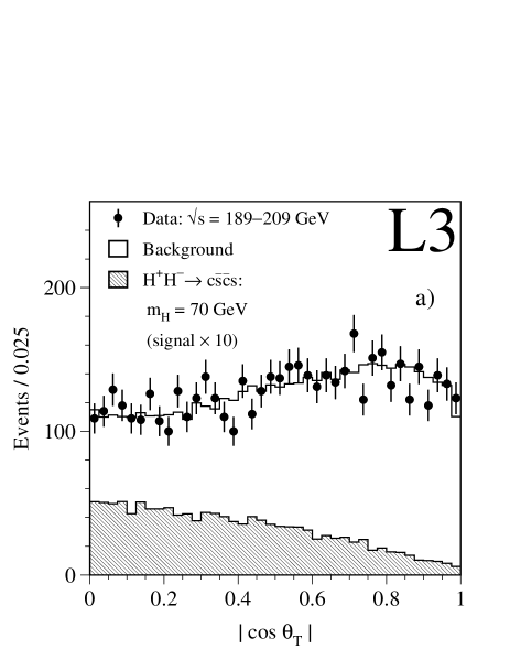
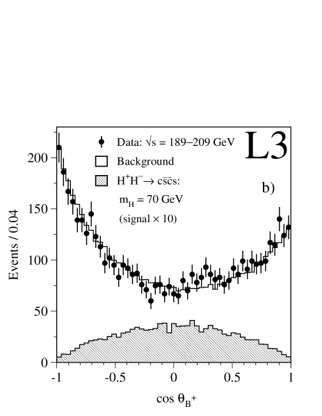
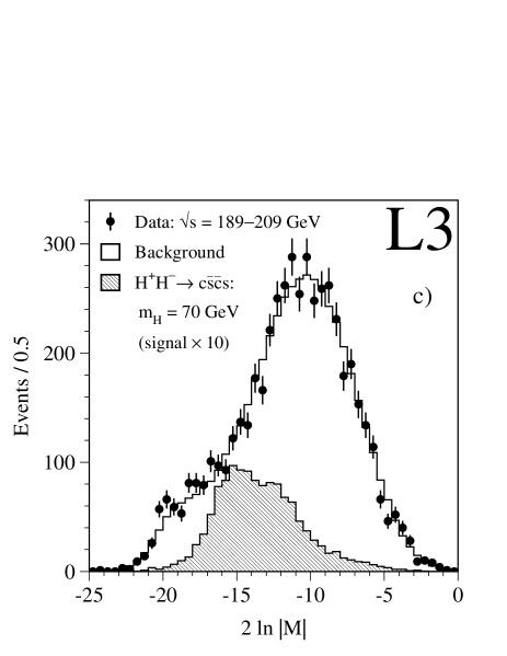
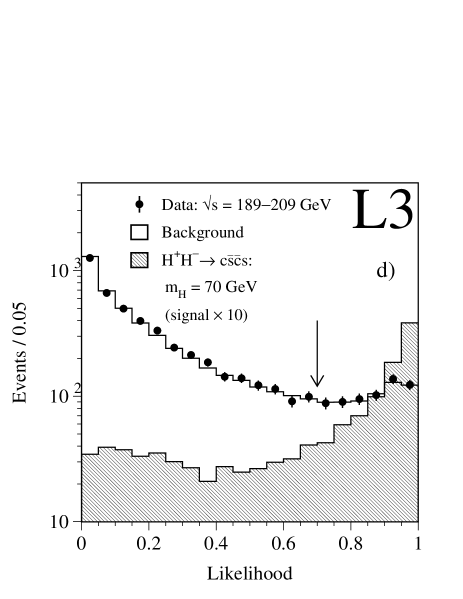
Figure 1: Distributions for the $\mathrm{\Hp\Hm\ra\mathrm{c\bar{s}\bar{c}s}}$ channel of: a) the absolute value of the cosine of the polar angle of the thrust axis, b) the cosine of the polar angle of the positively charged boson, c) the logarithm of the squared matrix element for the $\epem\ra\Wp\Wm$ process and d) the selection likelihood for $m_{\mathrm{\Hpm}}=70\,\GeV{}$. The points represent the data and the open histogram the expected background. The hatched histogram indicates the expected distribution for a signal with $m_{\mathrm{\Hpm}}=70\,\GeV{}$ and $\mathrm{Br(H^{\pm}\ra\tau\nu)}=0$, multiplied by a factor of 10. The arrow in d) shows the position of the cut.

Figures 1a, 1b and 1c show the distributions of the last three variables while Figure 1d presents the distribution of the likelihood variable for $m_{\mathrm{\Hpm}}=70\,\GeV$. A cut at 0.7 on this variable, which maximizes the signal sensitivity, is applied as a final selection criterion, for all mass hypotheses. The numbers of observed and expected events are given in Table 2 and the selection efficiencies in Table 3. The main contributions to the background come from hadronic W-pair decays (70%) and from the $\ee\ra\qqbar(\gamma)$ process (26%). Figure 2 shows the 5C mass of the pair-produced bosons before and after the cut on the final likelihoods. Peaks from pair-production of W as well as Z bosons are visible.

Search in the $\mathrm{\Hp\Hm\ra\mathrm{c\bar{s}\tau^{-}\nbar_{\tau}}}$ channel

The search in the $\mathrm{\Hp\Hm\ra\mathrm{c\bar{s}\tau^{-}\nbar_{\tau}}}$ channel selects events with high multiplicity, two hadronic jets and a tau candidate. Tau candidates can be identified either as electrons or muons with momentum incompatible with that expected for leptons originating from direct semileptonic decay of W pairs, or with narrow, low multiplicity jets with at least one charged track, singled out from the hadronic background with a neural network [18]. The tau energy is reconstructed by imposing four-momentum conservation and enforcing the hypothesis of the production of two equal mass particles. The events must have a transverse missing momentum of at least 20  and the absolute value of the cosine of the polar angle of the missing momentum is required to be less than 0.9. Finally, the di-jet invariant mass is required to be less than 100  and the mass recoiling against the di-jet system less than 130 , thus selecting 1026 events in data while 979 are expected from Standard Model processes, mainly from W pair-production where one of the W bosons decays into leptons and the other into hadrons. The signal efficiency is about 50%.

To discriminate the signal from the background, mass dependent likelihoods [20] are built which contain eight variables:

• the di-jet acoplanarity;

• the angle of the tau flight direction with respect to that of its parent boson in the rest frame of the latter;

• the di-jet mass;

• the quantity $2\ln|M|$ calculated using the four-momenta of the reconstructed jets and tau as well as the missing momentum and energy;

• the transverse momentum of the event, normalised to $\sqrt{s}$;

• the polar angle of the hadronic system, multiplied by the charge of the reconstructed tau;

• the sum $\Sigma_{\theta}$ of the angles between the tau candidate and the nearest jet and between the missing momentum and the nearest jet;

• the energy of the tau candidate, calculated in the rest frame of its parent boson and scaled by $\sqrt{s}$.

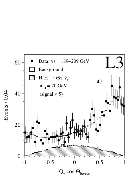
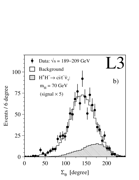
Figure 3: Distribution for the $\mathrm{\Hp\Hm\ra\mathrm{c\bar{s}\tau^{-}\nbar_{\tau}}}$ channel of: a) the cosine of the polar angle of the hadron system multiplied by the charge of the tau candidate, b) the sum of the angles between the tau candidate and the nearest jet and between the missing momentum and the nearest jet, c) the scaled energy of the tau candidate in the rest frame of the parent boson and d) the selection likelihood for $m_{\mathrm{\Hpm}}=70\,\GeV{}$. The points represent the data and the open histogram the expected background. The hatched histogram indicates the expected distribution for $m_{\mathrm{\Hpm}}=70\,\GeV{}$ and $\mathrm{Br(H^{\pm}\ra\tau\nu)}=0.5$, multiplied by a factor of 5. The arrow in d) shows the position of the cut.

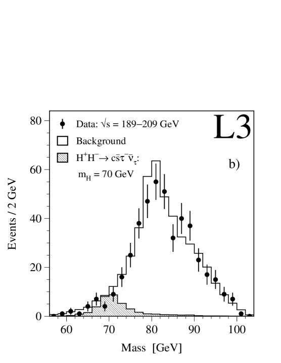
Figure 4: Reconstructed mass spectra in the $\mathrm{\Hp\Hm\ra\mathrm{c\bar{s}\tau^{-}\nbar_{\tau}}}$ channel, for data and expected background, for events a) before, and b) after, the cut on the likelihoods. The points represent the data and the open histogram the expected background. The expected distribution for $m_{\mathrm{\Hpm}}=70\,\GeV$ and $\mathrm{Br(H^{\pm}\ra\tau\nu)}=0.5$ is shown as the hatched histogram.

The distributions of the last three variables are shown in Figures 3a, 3b and 3c. Figure 3d presents an example of the distributions of the likelihood variable for $m_{\mathrm{\Hpm}}=70\,\GeV$ for data, background and signal Monte Carlo. A cut at 0.6 is applied for all likelihoods. This cut corresponds to the largest sensitivity to a charged Higgs signal. Table 2 gives the numbers of observed and expected events, while the selection efficiencies are given in Table 3. Over 95% of the background is due to W pair-production. Figure 4 shows the reconstructed mass of the pair-produced bosons before and after the cut on the final likelihoods.

Search in the $\mathrm{\Hp\Hm\ra\mathrm{\tau^{+}\nu_{\tau}\tau^{-}\nbar_{\tau}}}$ channel

The signature for the leptonic decay channel is a pair of tau leptons. These are identified either via their decay into electrons or muons, or as narrow jets.

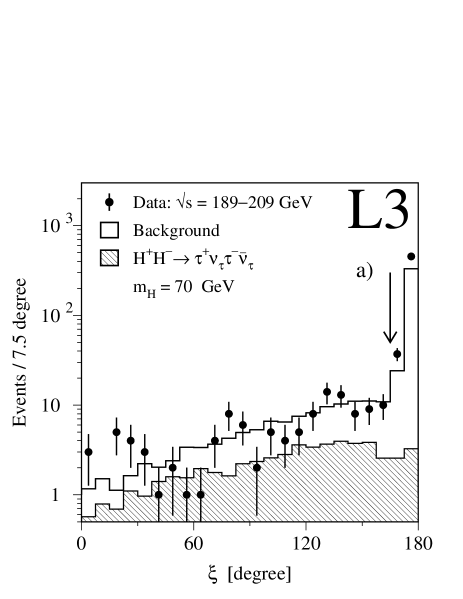
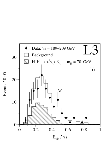
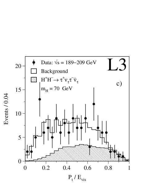
Figure 5: Distribution for the $\mathrm{\Hp\Hm\ra\mathrm{\tau^{+}\nu_{\tau}\tau^{-}\nbar_{\tau}}}$ channel of: a) the event collinearity angle, $\xi$, b) the scaled visible energy and c) the normalised transverse missing momentum of the event. In a) and b) all other selection criteria are applied and the arrows indicate the cut on the displayed variable. The points represent the data and the open histogram the expected background. The hatched histograms indicate the expected signal distributions for $m_{\mathrm{\Hpm}}=70\,\GeV{}$ and $\mathrm{Br(H^{\pm}\ra\tau\nu)}=1$.

The selection criteria are similar to those used at lower $\sqrt{s}$ [6, 7]. Low multiplicity events with large missing energy and momentum are retained. To reduce lepton-pair background, an upper cut is placed on the value of the event collinearity angle, $\xi$, defined as the maximum angle between any pair of tracks. The distribution of this variable is shown in Figure 5a. The contribution from cosmic muons is reduced by making use of information from the time-of-flight system. Figure 5b presents the distribution of the scaled visible energy, $E_{vis}/\sqrt{s}$, for events on which all other selection criteria are applied.

The analysis is modified with respect to those previously published [6, 7] in that the normalised transverse missing momentum of the event, ${P_{t}/E_{vis}}$, whose distribution is shown in Figure 5c, is used as a linear discriminant variable on which no cut is applied.

The efficiency of the $\mathrm{\Hp\Hm\ra\mathrm{\tau^{+}\nu_{\tau}\tau^{-}\nbar_{\tau}}}$ selection for several Higgs masses is listed in Table 3. The numbers of observed and expected events are presented in Table 2. The background is mainly formed by W-pair production (60%), two-photon interactions (26%) and lepton pair-production (9%).

Results

The number of selected events in each decay channel is consistent with the number of events expected from Standard Model processes. A technique based on a log-likelihood ratio [4] is used to calculate a confidence level (CL) that the observed events are consistent with background expectations. For the $\mathrm{c\bar{s}\bar{c}s}$ and $\mathrm{c\bar{s}\tau^{-}\nbar_{\tau}}$ channels, the reconstructed mass distributions, shown in Figures 2b and 4b, are used in the calculation, whereas for the $\mathrm{\tau^{+}\nu_{\tau}\tau^{-}\nbar_{\tau}}$ channel, the distribution of the normalised transverse missing momentum, shown in Figure 5c, is used.

The systematic uncertainties on the background level and the signal efficiencies are included in the confidence level calculation. These are due to finite Monte Carlo statistics and to the uncertainty on the background normalisation. The former uncertainty is 5% for the background and 2% for the signal Monte Carlo samples. The uncertainty on the background normalisation is 3% for the $\mathrm{\Hp\Hm\ra\mathrm{c\bar{s}\bar{c}s}}$ channel and 2% for the $\mathrm{c\bar{s}\tau^{-}\nbar_{\tau}}$ and $\mathrm{\tau^{+}\nu_{\tau}\tau^{-}\nbar_{\tau}}$ channels. The systematic uncertainty on the signal efficiency due to the selection procedure is estimated by varying the selection criteria and is found to be less than 1%. These systematic uncertainties decrease the $m_{\mathrm{\Hpm}}$ sensitivity of the combined analysis by about 200 .

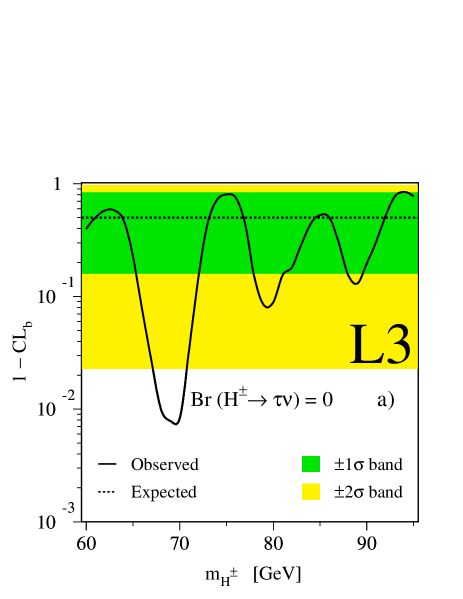
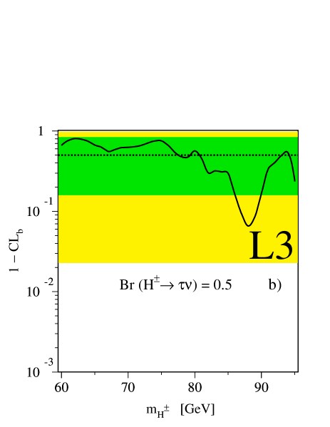
Figure 6: The background confidence level, $1-{CL_{b}}$, as a function of $m_{\mathrm{\Hpm}}$ for the data (solid line) and for the expectation in the absence of a signal (dashed line), for three values of the $\mathrm{H^{\pm}\ra\tau\nu}$ branching ratio. The shaded areas represent the symmetric $1\sigma$ and $2\sigma$ probability bands expected in the absence of a signal.

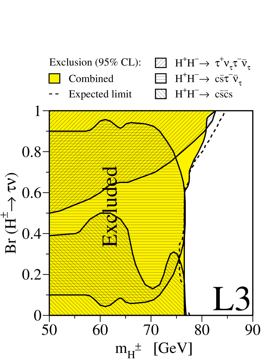
Figure 7: Excluded regions for the charged Higgs boson in the plane of the $\mathrm{H^{\pm}\ra\tau\nu}$ branching fraction versus mass, for the analyses of each final state and their combination. The dashed line indicates the median expected limit in the absence of a signal. Regions below $m_{\mathrm{\Hpm}}=50\,\GeV$ are excluded by data collected at the Z resonance [23] and at $\sqrt{s}=130-183\GeV$ [7].

Figure 6 compares the resulting background confidence level, $1-{CL_{b}}$, for the data to the expectation in the absence of a signal, for three values of the $\mathrm{H^{\pm}\ra\tau\nu}$ branching ratio: $\mathrm{Br(H^{\pm}\ra\tau\nu)}$ = 0, 0.5 and 1. The 68.3% and 95.4% probability bands expected in the absence of a signal are also displayed and denoted as $1\sigma$ and $2\sigma$, respectively. A slight excess of data appears around $m_{\mathrm{\Hpm}}=69$  for $\mathrm{Br(H^{\pm}\ra\tau\nu)}=0$, as previously observed [6]. It is compatible with a $2.5\sigma$ upward fluctuation in the background. The excess is also compatible with a $2.9\sigma$ downward fluctuation of the signal. As observed in Figures 6b and 6c, no excess is present in the $\mathrm{c\bar{s}\tau^{-}\nbar_{\tau}}$ and $\mathrm{\tau^{+}\nu_{\tau}\tau^{-}\nbar_{\tau}}$ channels around $m_{\mathrm{\Hpm}}=69$ . Therefore, the $\mathrm{c\bar{s}\bar{c}s}$ excess is interpreted as a statistical fluctuation in the background and lower limits at the 95% CL on $m_{\mathrm{\Hpm}}$ are derived [4] as a function of $\mathrm{Br(H^{\pm}\ra\tau\nu)}$. Data at $\sqrt{s}=130-183\,\GeV$ [7] are included to obtain the limits. Figure 7 shows the excluded $m_{\mathrm{\Hpm}}$ regions for each of the final states and their combination, as a function of $\mathrm{Br(H^{\pm}\ra\tau\nu)}$. Table 4 gives the observed and the median expected lower limits for several values of the branching ratio.

In conclusion, refined analyses and larger centre-of-mass energies improve the sensitivity of the search for charged Higgs bosons produced in $\epem$ collisions as compared to previous results [6, 7]. No significant excess is observed in data and a lower limit at 95% CL on the charged Higgs boson mass is obtained as

$$m_{\mathrm{\Hpm}}>76.5\,\GeV{},$$

independent of its branching ratio.

10

Author List

The L3 Collaboration:

P.Achard,²⁰ O.Adriani,¹⁷ M.Aguilar-Benitez,²⁴ J.Alcaraz,²⁴ G.Alemanni,²² J.Allaby,¹⁸ A.Aloisio,²⁸ M.G.Alviggi,²⁸ H.Anderhub,⁴⁶ V.P.Andreev,^6,33 F.Anselmo,⁸ A.Arefiev,²⁷ T.Azemoon,³ T.Aziz,⁹ P.Bagnaia,³⁸ A.Bajo,²⁴ G.Baksay,²⁵ L.Baksay,²⁵ S.V.Baldew,² S.Banerjee,⁹ Sw.Banerjee,⁴ A.Barczyk,^46,44 R.Barillère,¹⁸ P.Bartalini,²² M.Basile,⁸ N.Batalova,⁴³ R.Battiston,³² A.Bay,²² F.Becattini,¹⁷ U.Becker,¹³ F.Behner,⁴⁶ L.Bellucci,¹⁷ R.Berbeco,³ J.Berdugo,²⁴ P.Berges,¹³ B.Bertucci,³² B.L.Betev,⁴⁶ M.Biasini,³² M.Biglietti,²⁸ A.Biland,⁴⁶ J.J.Blaising,⁴ S.C.Blyth,³⁴ G.J.Bobbink,² A.Böhm,¹ L.Boldizsar,¹² B.Borgia,³⁸ S.Bottai,¹⁷ D.Bourilkov,⁴⁶ M.Bourquin,²⁰ S.Braccini,²⁰ J.G.Branson,⁴⁰ F.Brochu,⁴ J.D.Burger,¹³ W.J.Burger,³² X.D.Cai,¹³ M.Capell,¹³ G.Cara Romeo,⁸ G.Carlino,²⁸ A.Cartacci,¹⁷ J.Casaus,²⁴ F.Cavallari,³⁸ N.Cavallo,³⁵ C.Cecchi,³² M.Cerrada,²⁴ M.Chamizo,²⁰ Y.H.Chang,⁴⁸ M.Chemarin,²³ A.Chen,⁴⁸ G.Chen,⁷ G.M.Chen,⁷ H.F.Chen,²¹ H.S.Chen,⁷ G.Chiefari,²⁸ L.Cifarelli,³⁹ F.Cindolo,⁸ I.Clare,¹³ R.Clare,³⁷ G.Coignet,⁴ N.Colino,²⁴ S.Costantini,³⁸ B.de la Cruz,²⁴ S.Cucciarelli,³² J.A.van Dalen,³⁰ R.de Asmundis,²⁸ P.Déglon,²⁰ J.Debreczeni,¹² A.Degré,⁴ K.Dehmelt,²⁵ K.Deiters,⁴⁴ D.della Volpe,²⁸ E.Delmeire,²⁰ P.Denes,³⁶ F.DeNotaristefani,³⁸ A.De Salvo,⁴⁶ M.Diemoz,³⁸ M.Dierckxsens,² C.Dionisi,³⁸ M.Dittmar,⁴⁶ A.Doria,²⁸ M.T.Dova,^10,♯ D.Duchesneau,⁴ M.Duda,¹ B.Echenard,²⁰ A.Eline,¹⁸ A.El Hage,¹ H.El Mamouni,²³ A.Engler,³⁴ F.J.Eppling,¹³ P.Extermann,²⁰ M.A.Falagan,²⁴ S.Falciano,³⁸ A.Favara,³¹ J.Fay,²³ O.Fedin,³³ M.Felcini,⁴⁶ T.Ferguson,³⁴ H.Fesefeldt,¹ E.Fiandrini,³² J.H.Field,²⁰ F.Filthaut,³⁰ P.H.Fisher,¹³ W.Fisher,³⁶ I.Fisk,⁴⁰ G.Forconi,¹³ K.Freudenreich,⁴⁶ C.Furetta,²⁶ Yu.Galaktionov,^27,13 S.N.Ganguli,⁹ P.Garcia-Abia,²⁴ M.Gataullin,³¹ S.Gentile,³⁸ S.Giagu,³⁸ Z.F.Gong,²¹ G.Grenier,²³ O.Grimm,⁴⁶ M.W.Gruenewald,¹⁶ M.Guida,³⁹ R.van Gulik,² V.K.Gupta,³⁶ A.Gurtu,⁹ L.J.Gutay,⁴³ D.Haas,⁵ D.Hatzifotiadou,⁸ T.Hebbeker,¹ A.Hervé,¹⁸ J.Hirschfelder,³⁴ H.Hofer,⁴⁶ M.Hohlmann,²⁵ G.Holzner,⁴⁶ S.R.Hou,⁴⁸ Y.Hu,³⁰ B.N.Jin,⁷ L.W.Jones,³ P.de Jong,² I.Josa-Mutuberría,²⁴ D.Käfer,¹ M.Kaur,¹⁴ M.N.Kienzle-Focacci,²⁰ J.K.Kim,⁴² J.Kirkby,¹⁸ W.Kittel,³⁰ A.Klimentov,^13,27 A.C.König,³⁰ M.Kopal,⁴³ V.Koutsenko,^13,27 M.Kräber,⁴⁶ R.W.Kraemer,³⁴ A.Krüger,⁴⁵ A.Kunin,¹³ P.Ladron de Guevara,²⁴ I.Laktineh,²³ G.Landi,¹⁷ M.Lebeau,¹⁸ A.Lebedev,¹³ P.Lebrun,²³ P.Lecomte,⁴⁶ P.Lecoq,¹⁸ P.Le Coultre,⁴⁶ J.M.Le Goff,¹⁸ R.Leiste,⁴⁵ M.Levtchenko,²⁶ P.Levtchenko,³³ C.Li,²¹ S.Likhoded,⁴⁵ C.H.Lin,⁴⁸ W.T.Lin,⁴⁸ F.L.Linde,² L.Lista,²⁸ Z.A.Liu,⁷ W.Lohmann,⁴⁵ E.Longo,³⁸ Y.S.Lu,⁷ C.Luci,³⁸ L.Luminari,³⁸ W.Lustermann,⁴⁶ W.G.Ma,²¹ L.Malgeri,²⁰ A.Malinin,²⁷ C.Maña,²⁴ J.Mans,³⁶ J.P.Martin,²³ F.Marzano,³⁸ K.Mazumdar,⁹ R.R.McNeil,⁶ S.Mele,^18,28 L.Merola,²⁸ M.Meschini,¹⁷ W.J.Metzger,³⁰ A.Mihul,¹¹ H.Milcent,¹⁸ G.Mirabelli,³⁸ J.Mnich,¹ G.B.Mohanty,⁹ G.S.Muanza,²³ A.J.M.Muijs,² B.Musicar,⁴⁰ M.Musy,³⁸ S.Nagy,¹⁵ S.Natale,²⁰ M.Napolitano,²⁸ F.Nessi-Tedaldi,⁴⁶ H.Newman,³¹ A.Nisati,³⁸ T.Novak,³⁰ H.Nowak,⁴⁵ R.Ofierzynski,⁴⁶ G.Organtini,³⁸ I.Pal,⁴³C.Palomares,²⁴ P.Paolucci,²⁸ R.Paramatti,³⁸ G.Passaleva,¹⁷ S.Patricelli,²⁸ T.Paul,¹⁰ M.Pauluzzi,³² C.Paus,¹³ F.Pauss,⁴⁶ M.Pedace,³⁸ S.Pensotti,²⁶ D.Perret-Gallix,⁴ B.Petersen,³⁰ D.Piccolo,²⁸ F.Pierella,⁸ M.Pioppi,³² P.A.Piroué,³⁶ E.Pistolesi,²⁶ V.Plyaskin,²⁷ M.Pohl,²⁰ V.Pojidaev,¹⁷ J.Pothier,¹⁸ D.Prokofiev,³³ J.Quartieri,³⁹ G.Rahal-Callot,⁴⁶ M.A.Rahaman,⁹ P.Raics,¹⁵ N.Raja,⁹ R.Ramelli,⁴⁶ P.G.Rancoita,²⁶ R.Ranieri,¹⁷ A.Raspereza,⁴⁵ P.Razis,²⁹D.Ren,⁴⁶ M.Rescigno,³⁸ S.Reucroft,¹⁰ S.Riemann,⁴⁵ K.Riles,³ B.P.Roe,³ L.Romero,²⁴ A.Rosca,⁴⁵ C.Rosenbleck,¹ S.Rosier-Lees,⁴ S.Roth,¹ J.A.Rubio,¹⁸ G.Ruggiero,¹⁷ H.Rykaczewski,⁴⁶ A.Sakharov,⁴⁶ S.Saremi,⁶ S.Sarkar,³⁸ J.Salicio,¹⁸ E.Sanchez,²⁴ C.Schäfer,¹⁸ V.Schegelsky,³³ H.Schopper,⁴⁷ D.J.Schotanus,³⁰ C.Sciacca,²⁸ L.Servoli,³² S.Shevchenko,³¹ N.Shivarov,⁴¹ V.Shoutko,¹³ E.Shumilov,²⁷ A.Shvorob,³¹ D.Son,⁴² C.Souga,²³ P.Spillantini,¹⁷ M.Steuer,¹³ D.P.Stickland,³⁶ B.Stoyanov,⁴¹ A.Straessner,²⁰ K.Sudhakar,⁹ G.Sultanov,⁴¹ L.Z.Sun,²¹ S.Sushkov,¹ H.Suter,⁴⁶ J.D.Swain,¹⁰ Z.Szillasi,^25,¶ X.W.Tang,⁷ P.Tarjan,¹⁵ L.Tauscher,⁵ L.Taylor,¹⁰ B.Tellili,²³ D.Teyssier,²³ C.Timmermans,³⁰ Samuel C.C.Ting,¹³ S.M.Ting,¹³ S.C.Tonwar,⁹ J.Tóth,¹² C.Tully,³⁶ K.L.Tung,⁷J.Ulbricht,⁴⁶ E.Valente,³⁸ R.T.Van de Walle,³⁰ R.Vasquez,⁴³ V.Veszpremi,²⁵ G.Vesztergombi,¹² I.Vetlitsky,²⁷ D.Vicinanza,³⁹ G.Viertel,⁴⁶ S.Villa,³⁷ M.Vivargent,⁴ S.Vlachos,⁵ I.Vodopianov,²⁵ H.Vogel,³⁴ H.Vogt,⁴⁵ I.Vorobiev,^34,27 A.A.Vorobyov,³³ M.Wadhwa,⁵ Q.Wang³⁰ X.L.Wang,²¹ Z.M.Wang,²¹ M.Weber,¹ P.Wienemann,¹ H.Wilkens,³⁰ S.Wynhoff,³⁶ L.Xia,³¹ Z.Z.Xu,²¹ J.Yamamoto,³ B.Z.Yang,²¹ C.G.Yang,⁷ H.J.Yang,³ M.Yang,⁷ S.C.Yeh,⁴⁹ An.Zalite,³³ Yu.Zalite,³³ Z.P.Zhang,²¹ J.Zhao,²¹ G.Y.Zhu,⁷ R.Y.Zhu,³¹ H.L.Zhuang,⁷ A.Zichichi,^8,18,19 B.Zimmermann,⁴⁶ M.Zöller.¹

• III. Physikalisches Institut, RWTH, D-52056 Aachen, Germany^§

• National Institute for High Energy Physics, NIKHEF, and University of Amsterdam, NL-1009 DB Amsterdam, The Netherlands

• University of Michigan, Ann Arbor, MI 48109, USA

• Laboratoire d’Annecy-le-Vieux de Physique des Particules, LAPP,IN2P3-CNRS, BP 110, F-74941 Annecy-le-Vieux CEDEX, France

• Institute of Physics, University of Basel, CH-4056 Basel, Switzerland

• Louisiana State University, Baton Rouge, LA 70803, USA

• Institute of High Energy Physics, IHEP, 100039 Beijing, China^△

• University of Bologna and INFN-Sezione di Bologna, I-40126 Bologna, Italy

• Tata Institute of Fundamental Research, Mumbai (Bombay) 400 005, India

• Northeastern University, Boston, MA 02115, USA

• Institute of Atomic Physics and University of Bucharest, R-76900 Bucharest, Romania

• Central Research Institute for Physics of the Hungarian Academy of Sciences, H-1525 Budapest 114, Hungary^‡

• Massachusetts Institute of Technology, Cambridge, MA 02139, USA

• Panjab University, Chandigarh 160 014, India.

• KLTE-ATOMKI, H-4010 Debrecen, Hungary^¶

• Department of Experimental Physics, University College Dublin, Belfield, Dublin 4, Ireland

• INFN Sezione di Firenze and University of Florence, I-50125 Florence, Italy

• European Laboratory for Particle Physics, CERN, CH-1211 Geneva 23, Switzerland

• World Laboratory, FBLJA Project, CH-1211 Geneva 23, Switzerland

• University of Geneva, CH-1211 Geneva 4, Switzerland

• Chinese University of Science and Technology, USTC, Hefei, Anhui 230 029, China^△

• University of Lausanne, CH-1015 Lausanne, Switzerland

• Institut de Physique Nucléaire de Lyon, IN2P3-CNRS,Université Claude Bernard, F-69622 Villeurbanne, France

• Centro de Investigaciones Energéticas, Medioambientales y Tecnológicas, CIEMAT, E-28040 Madrid, Spain${\flat}$

• Florida Institute of Technology, Melbourne, FL 32901, USA

• INFN-Sezione di Milano, I-20133 Milan, Italy

• Institute of Theoretical and Experimental Physics, ITEP, Moscow, Russia

• INFN-Sezione di Napoli and University of Naples, I-80125 Naples, Italy

• Department of Physics, University of Cyprus, Nicosia, Cyprus

• University of Nijmegen and NIKHEF, NL-6525 ED Nijmegen, The Netherlands

• California Institute of Technology, Pasadena, CA 91125, USA

• INFN-Sezione di Perugia and Università Degli Studi di Perugia, I-06100 Perugia, Italy

• Nuclear Physics Institute, St. Petersburg, Russia

• Carnegie Mellon University, Pittsburgh, PA 15213, USA

• INFN-Sezione di Napoli and University of Potenza, I-85100 Potenza, Italy

• Princeton University, Princeton, NJ 08544, USA

• University of Californa, Riverside, CA 92521, USA

• INFN-Sezione di Roma and University of Rome, “La Sapienza”, I-00185 Rome, Italy

• University and INFN, Salerno, I-84100 Salerno, Italy

• University of California, San Diego, CA 92093, USA

• Bulgarian Academy of Sciences, Central Lab. of Mechatronics and Instrumentation, BU-1113 Sofia, Bulgaria

• The Center for High Energy Physics, Kyungpook National University, 702-701 Taegu, Republic of Korea

• Purdue University, West Lafayette, IN 47907, USA

• Paul Scherrer Institut, PSI, CH-5232 Villigen, Switzerland

• DESY, D-15738 Zeuthen, Germany

• Eidgenössische Technische Hochschule, ETH Zürich, CH-8093 Zürich, Switzerland

• University of Hamburg, D-22761 Hamburg, Germany

• National Central University, Chung-Li, Taiwan, China

• Department of Physics, National Tsing Hua University, Taiwan, China

• Supported by the German Bundesministerium für Bildung, Wissenschaft, Forschung und Technologie

• Supported by the Hungarian OTKA fund under contract numbers T019181, F023259 and T037350.

• Also supported by the Hungarian OTKA fund under contract number T026178.

• Supported also by the Comisión Interministerial de Ciencia y Tecnología.

• Also supported by CONICET and Universidad Nacional de La Plata, CC 67, 1900 La Plata, Argentina.

• Supported by the National Natural Science Foundation of China.

$\sqrt{s}$ ()	188.6	191.6	195.5	199.5	201.7	204.9	206.4	208.0
Luminosity (pb-1)	176.8	029.8	084.2	083.3	037.2	079.0	130.8	008.3

Table 1: Average centre-of-mass energies and corresponding integrated luminosities.

	Channel
	$\mathrm{c\bar{s}\bar{c}s}$	$\mathrm{c\bar{s}\tau^{-}\nbar_{\tau}}$	$\mathrm{\tau^{+}\nu_{\tau}\tau^{-}\nbar_{\tau}}$
Data	2296	442	141
Background	2228	464	141
Signal	0100	076	050

Table 2: Number of observed data events and background expectations in the three analysis channels. The uncertainty on the background expectations is estimated to be 5%. The numbers of expected signal events for $m_{\mathrm{\Hpm}}=70\,\GeV$ and $\mathrm{Br(H^{\pm}\ra\tau\nu)}=0$, 0.5 and 1 are also given for the $\mathrm{c\bar{s}\bar{c}s}$, $\mathrm{c\bar{s}\tau^{-}\nbar_{\tau}}$ and $\mathrm{\tau^{+}\nu_{\tau}\tau^{-}\nbar_{\tau}}$ channels, respectively.

Channel	Selection efficiency (%)
	$m_{\mathrm{\Hpm}}=$	60	70	80	90	95
$\mathrm{c\bar{s}\bar{c}s}$		62	62	50	58	64
$\mathrm{c\bar{s}\tau^{-}\nbar_{\tau}}$		38	51	43	43	39
$\mathrm{\tau^{+}\nu_{\tau}\tau^{-}\nbar_{\tau}}$		26	30	33	34	36

Table 3: Selection efficiencies for various charged Higgs masses. The efficiencies are largely independent of the centre-of-mass energy. The uncertainty on each efficiency is estimated to be 2%.

$\mathrm{Br(H^{\pm}\ra\tau\nu)}$	Lower limits () at 95% CL
	observed	expected
0.00	76.7	77.5
0.26	76.5	75.6
0.50	76.6	76.5
1.00	82.7	84.6

Table 4: Observed and expected lower limits at 95% CL for different values of the $\mathrm{H^{\pm}\ra\tau\nu}$ branching ratio. The minimum observed limit is at $\mathrm{Br(H^{\pm}\ra\tau\nu)}=0.26$.

Figure 2: Reconstructed mass spectra in the $\mathrm{\Hp\Hm\ra\mathrm{c\bar{s}\bar{c}s}}$ channel, for data and expected background, for events a) before, and b) after, the cut on the likelihoods. The points represent the data and the open histogram the expected background. The expected distribution for $m_{\mathrm{\Hpm}}=70\,\GeV{}$ and $\mathrm{Br(H^{\pm}\ra\tau\nu)}=0$ is shown as the hatched histogram.

References

- [1] S.L. Glashow, \NP22 (1961) 579; S. Weinberg, \PRL19 (1967) 1264; A. Salam, Elementary Particle Theory, edited by N. Svartholm (Almqvist and Wiksell, Stockholm, 1968), p. 367
- [2] P.W. Higgs, \PL12 (1964) 132, \PRL13 (1964) 508; \PR145 (1966) 1156; F. Englert and R. Brout, \PRL13 (1964) 321; G.S. Guralnik, C.R. Hagen and T.W.B. Kibble, Phys. Rev. Lett. 13 (1964) 585
- [3] L3 Collab., P. Achard \etal, Phys. Lett. B 517 (2001) 319
- [4] ALEPH, DELPHI, L3 and OPAL Collab., The LEP Working Group for Higgs Boson Searches, \PLB 565 (2003) 61
- [5] S. Dawson \etal, The Physics of the Higgs Bosons: Higgs Hunter’s Guide, Addison Wesley, Menlo Park, 1989
- [6] L3 Collab., M. Acciarri \etal, Phys. Lett. B 466 (1999) 71; L3 Collab., M. Acciarri \etal, Phys. Lett. B 496 (2000) 34
- [7] L3 Collab., M. Acciarri \etal, Phys. Lett. B 446 (1999) 368
- [8] ALEPH Collab., A. Heister \etal, Phys. Lett. B 543 (2002) 1; DELPHI Collab., J. Abdallah \etal, Phys. Lett. B 525 (2002) 17; OPAL Collab., G. Abbiendi \etal, Eur. Phys. J. C 7 (1999) 407
- [9] L3 Collab., B. Adeva \etal, Nucl. Instr. Meth. A 289 (1990) 35; J.A. Bakken \etal, Nucl. Instr. Meth. A 275 (1989) 81; O. Adriani \etal, Nucl. Instr. Meth. A 302 (1991) 53; B. Adeva \etal, Nucl. Instr. Meth. A 323 (1992) 109; K. Deiters \etal, Nucl. Instr. Meth. A 323 (1992) 162; M. Chemarin \etal, Nucl. Instr. Meth. A 349 (1994) 345; M. Acciarri \etal, Nucl. Instr. Meth. A 351 (1994) 300; G. Basti \etal, Nucl. Instr. Meth. A 374 (1996) 293; A. Adam \etal, Nucl. Instr. Meth. A 383 (1996) 342; O. Adriani \etal, Phys. Rep. 236 (1993) 1
- [10] HZHA version 2 is used; P. Janot, in Physics at LEP2, ed. G. Altarelli, T. Sjöstrand and F. Zwirner, (CERN 96-01, 1996), volume 2, p. 309
- [11] PYTHIA version 5.722 is used; T. Sjöstrand, preprint CERN-TH/7112/93 (1993), revised 1995; Comp. Phys. Comm. 82 (1994) 74
- [12] KK2f version 4.14 is used; S. Jadach, B.F.L. Ward and Z. Wa̧s, Comp. Phys. Comm 130 (2000) 260
- [13] BHWIDE version 1.03 is used; S. Jadach, W. Placzek and B.F.L. Ward, Phys. Lett. B 390 (1997) 298
- [14] YFSWW version 1.14 is used; S. Jadach \etal, Phys. Rev. D 54 (1996) 5434; Phys. Lett. B 417 (1998) 326; Phys. Rev. D 61 (2000) 113010; Phys. Rev. D 65 (2002) 093010
- [15] PHOJET version 1.05 is used; R. Engel, Z. Phys. C 66 (1995) 203; R. Engel and J. Ranft, Phys. Rev. D 54 (1996) 4244
- [16] DIAG 36 Monte Carlo; F.A. Berends, P.H. Daverfeldt and R. Kleiss, \NPB 253 (1985) 441
- [17] GEANT version 3.15 is used;R. Brun \etal, preprint CERN DD/EE/84-1 (1985), revised 1987. The GHEISHA program (H. Fesefeldt, RWTH Aachen Report PITHA 85/02, 1985) is used to simulate hadronic interactions
- [18] L3 Collab., P. Achard \etal, Measurement of the cross section of W pair-production at LEP, in preparation
- [19] S. Bethke \etal, Nucl. Phys. B 370 (1992) 390
- [20] L3 Collab., P. Achard \etal, Phys. Lett. B 545 (2002) 30
- [21] L3 Collab., M. Acciarri \etal, Phys. Lett. B 413 (1997) 176
- [22] EXCALIBUR version 1.11 is used; F.A. Berends, R. Kleiss and R. Pittau, Comp. Phys. Comm. 85 (1995) 437
- [23] L3 Collab., O. Adriani \etal, \PLB 294 (1992) 457; L3 Collab., O. Adriani \etal, \ZfPC 57 (1993) 355