LAL 03-53

RARE B DECAYS AND DIRECT CP VIOLATION AT BABAR Sandrine Laplace
On behalf of the BABAR Collaboration
Laboratoire de l’Accélérateur Linéaire,
IN2P3-CNRS et Université de Paris-Sud, BP 34, F-91898 Orsay Cedex, France

Abstract

The search for rare $B$ decays and direct $CP$ violation at BABAR is described. The following measurements (based on integrated luminosities ranging from $56.4$ to $81.9~{}fb^{-1}$) are summarized: the inclusive branching fractions and direct $CP$ asymmetries of $B^{+}\to h^{+}h^{-}h^{+}$ ($h=\pi,K$), the exclusive branching fractions of $B^{+}\to K^{+}\pi^{-}\pi^{+}$ (where significant signals are observed in the $B^{+}\to K^{*0}(892)\pi^{+}$, $B^{+}\to f_{0}(980)K^{+}$, $B^{+}\to\chi_{c0}K^{+}$, $B^{+}\to\overline{D}^{0}\pi^{+}$ and $B^{+}\to{\rm higher}~{}K^{*0}\pi^{+}$ channels), the branching fractions of $B^{+}\to\rho^{0}\rho^{+}$ and $B^{+}\to\rho^{0}K^{*+}$, and finally, the branching fractions, the longitudinal components, and the direct $CP$ asymmetries in $B\to\phi K^{*}$.

To appear in the proceedings of the 17th Les Rencontres de Physique de la Vallee d’Aoste:

Results and Perspectives in Particle Physics, La Thuile, Aosta Valley, Italy, 9-15 Mar 2003

1 Introduction

Measurements of the branching fractions and direct $CP$ asymmetries of rare $B$ decays using the BABAR detector[1] are presented. Rare $B$ decays can be classified according to their suppression factor:

• a small CKM matrix element, as for charmless $B$ decays which amplitudes are suppressed by a factor $|V_{ub}|/|V_{cb}|\simeq\lambda$ compared to charm $B$ decay amplitudes. Measurements related to the decays $B\to hhh$($h=\pi,~{}K$), $B\to\rho\rho$ and $B\to K^{*}\rho$ are presented.

• a dominant diagram involving a loop, which amplitudes are suppressed by either

  • $\alpha_{S}/4\pi$ for gluonic penguin ($b\to s~{}{\rm gluon}$) as in the exclusive decays $B\to\eta^{\prime}K^{*}$ and $B\to\phi K^{*}$.

  • $\alpha_{\rm QED}/4\pi$ for radiative penguins ($b\to s\gamma/d\gamma$), as in the exclusive decays $B\to K^{*}\gamma$ and $B\to\rho\gamma$ or the inclusive decay $b\to s\gamma$, and for electroweak penguins ($b\to sZ(l\bar{l})/s\gamma(l\bar{l})$), as in the exclusive decay $B\to K\nu\bar{\nu}$.

All the measurements mentioned above were presented in my talk, but only the results newly released during the winter conferences are detailed in these proceedings, i.e., $B\to hhh$($h=\pi,~{}K$), $B\to\rho\rho$, $B\to K^{*}\rho$ and $B\to\phi K^{*}$.

The motivation for such measurements is twofold: first, they could allow to see indirect effects of new physics particles virtually created in loop. Such effects may show up in different branching fractions and $CP$ asymmetries than those predicted by the Standard Model. One concentrates here on time-integrated direct $CP$ asymmetries. Time-dependent asymmetries are described elsewhere[2].

Time-integrated direct $CP$ asymmetries require at least two (Standard Model or New Physics) amplitudes contributing to a process with different weak and strong phases: calling $A$ the total amplitude of the process $B^{0}~{}(B^{+})\to f$ and $\bar{A}$ the one of the $CP$ conjugated process $\overline{B}^{0}~{}(B^{-})\to f$, one can split the amplitudes $A$ and $\bar{A}$ into a sum of real amplitudes $A_{k}$, $CP$-odd weak phases $\phi_{k}$ and $CP$-even strong phases $\delta_{k}$:

$$A=\sum_{k}A_{k}e^{i\phi_{k}}e^{i\delta_{k}},\quad\bar{A}=\sum_{k}A_{k}e^{-i\phi_{k}}e^{i\delta_{k}}.$$ (1)

The asymmetry between $A$ and $\bar{A}$ can then be written in terms of differences of weak and strong phases (the expression below is given in the case where two amplitudes contribute to the process):

$$|A|^{2}-|\bar{A}|^{2}=-4A_{1}A_{2}\sin(\phi_{1}-\phi_{2})\sin(\delta_{1}-\delta_{2}).$$ (2)

Beyond the search for hints of new physics, measurements of rare $B$ decays can help constraining the Standard Model unknown parameters. For example, time-dependent $CP$ asymmetries in $B\to\pi\pi$ and $B\to\eta^{\prime}K^{*}$, $B\to\phi K^{*}$ allow to measure $\sin 2\alpha$ and $\sin 2\beta$ where $\alpha$ and $\beta$ are two angles of the Unitarity Triangle; the ratio of the $B\to\rho\gamma$ and $B\to K^{*}\gamma$ rates constrains the ratio of CKM matrix elements $|V_{td}|/|V_{ts}|$; finally, the $b\to s\gamma$ spectrum helps to measure $V_{ub}$ and to constrain Heavy Quark Effective Theory parameters.

2 The BABAR detector and dataset

The BABAR detector is described elsewhere[1] in detail. It consists of a tracking system composed from a 5-layer double sided silicon micro strip vertex tracker (SVT) and from a 40-layer drift chamber (DCH), both operating in a $1.5$ T solenoidal magnetic field. Charged particle identification is mainly performed using a ring imaging Cherenkov detector (DIRC): the separation between kaons and pions ranges between $8\sigma$ for a momentum of $2~{}{\rm GeV/c^{2}}$ and $4\sigma$ for a momentum of $4~{}{\rm GeV/c^{2}}$. Photons and neutral hadrons are detected in a CsI(Tl) electromagnetic calorimeter. The identification of muons and neutral hadrons is done in the flux return instrumented with many layers of resistive plate chambers (IFR).

The data used in the analyses presented here were collected between 1999 and 2002. The total luminosity integrated at the $\Upsilon(4S)$ resonance (on-resonance data) is $81.9~{}fb^{-1}$, and the one integrated $40$ MeV below the $\Upsilon(4S)$ resonance (off-resonance data, used for continuum background studies) is $9.6~{}fb^{-1}$. Some of the analyses are performed on a fraction of the total integrated luminosity only.

3 Kinematics and event topology at a $B$ factory: background fighting

At the PEP-II $B$ factory, $B$ mesons are produced by colliding electrons and positrons at a center of mass energy equal to the $\Upsilon(4S)$ mass. At this energy, the $b\bar{b}$ cross-section corresponds to about $25\%$ of the total cross-section (including as well lighter quark production, called thereafter continuum). Continuum is a first source of background. Cross-talk from other $B$ decays is a second source of background referred to as $B$ background in the following.

The kinematic and topological variables described in this section are used to distinguish signal $B$ events from continuum and $B$ backgrounds.

3.1 Kinematic variables

The conservation of energy and momentum allows us to build the following two (nearly uncorrelated) kinematic variables:

• The variable $\Delta E$ is defined as:

  $$\Delta E=E^{*}_{B}-\sqrt{s}/2,$$ (3)

  where $E^{*}_{B}$ is the $B$ candidate energy and $\sqrt{s}$ is the beam energy, both calculated in the $\Upsilon(4S)$ center of mass. When the $B$ candidate corresponds to a real $B$ decay, $\Delta E$ is close from zero, up to the resolution which is dominated by the reconstruction of the $B$ energy (a few tens of MeV, depending on the nature of the daughters of the $B$).

• the energy-substituted mass, $m_{\rm ES}$, is defined by:

  $$m_{\rm ES}=\sqrt{(s/2+\vec{p}_{i}.\vec{p}_{B})^{2}/E_{i}^{2}-\vec{p}_{B}^{2}},$$ (4)

  where $E_{i}$ and $\vec{p}_{i}$ are respectively the total energy and the momentum of the $e^{+}e^{-}$ pair in the laboratory frame, and $\vec{p}_{B}$ is the momentum of the reconstructed $B$ candidate. For a real $B$ decay, $m_{\rm ES}$ peaks around the $B$ mass, up to the resolution of $2.6~{}{\rm MeV/c^{2}}$ dominated by the beam energy dispersion.

Kinematic variables are used both for continuum and $B$ background rejection. Because they are mostly uncorrelated, these two variables are often combined into a likelihood function.

3.2 Topological variables

At the $\Upsilon(4S)$ energy, $B^{0}{\kern-1.60004pt\kern 1.79993pt\overline{\kern-1.79993ptB}{}^{0}}$ pairs are produced almost at rest in the $\Upsilon(4S)$ center of mass. Therefore, in this frame, the $B$ daughters are isotropically distributed. Oppositely, for the lighter quarks (mainly for the $u,d,s$ quarks, to a lesser extend for the $c$ quark) extra energy is available to boost the produced particles, leading to a back-to-back jet structure.

Moreover, in the process $e^{+}e^{-}\to\Upsilon(4S)\to B{\kern-1.60004pt\overline{B}}$ where the spin-$1$ $\Upsilon(4S)$ decays into two spin-$0$ $B$ mesons, the angular distribution of the $B$ in the center of mass follows a $\sin^{2}\theta_{B}$ distribution where $\theta_{B}$ is the angle between the $B$ direction and the beam axis. Contrarily, in the process $e^{+}e^{-}\to f\bar{f}$ (where $f$ is a fermion), the distribution follows $1+\cos^{2}\theta_{T}$ where $\theta_{T}$ is the angle between the “jet direction” and the beam axis.

Topological variables can be built to take advantage of these shape properties. Amongst them, one can retain:

• ${\rm cos}\theta(T_{B},z)$: the cosine of the angle between the $B$ candidate thrust direction and the beam axis. True $B$ decays lead to a flat distribution, while one retrieve the $1+\cos^{2}\theta$ distribution mentioned earlier for continuum background.

• $L_{0}$ and $L_{2}$: momentum weighted monomials defined as:

  $$L_{n}=\sum_{i={\rm ROE}}p_{i}|{\rm cos}(\theta_{T_{B},i})|^{n}~{},$$ (5)

  where ${\rm cos}(\theta_{T_{B},i})$ is the cosine between the thrust direction of the $B$ candidate and the $i$-th track of the Rest Of the Event, ROE, (corresponding to what remains in the event once the $B$ candidate tracks are removed).

Because topological variables are related to $B$ decays and continuum production properties, they are mostly used for continuum background rejection, while being inefficient for $B$ background rejection.

Often highly correlated amongst each others, they are combined using Fisher[3] or neural network discriminants. Figure 1 shows the Fisher discriminant outputs using the variables $L_{0}$ and $L_{2}$ for $B^{0}\to\pi^{+}\pi^{-}$ Monte Carlo and continuum background. One obtains a good separation between these two categories of events.

Figure 1: Fisher discriminant output using the variables $L_{0}$ and $L_{2}$ (cf. Eq. 5) for Monte Carlo $B^{0}\to\pi^{+}\pi^{-}$ signal (dots) and continuum background (crosses).

4 Charmless $B$ decays

4.1 Inclusive rates and direct CP violation in $B^{+}\to h^{+}h^{-}h^{+}$ ($h=\pi,K$)

Measurements of the $B^{+}\to h^{+}h^{-}h^{+}$ ($h=\pi,K$) decays can be used to determine the Unitarity Triangle angle $\gamma$ and to help reducing uncertainties on the measurement of the angle $\alpha$[4]. Amongst the six final states considered here, two of them do not occur in first or second order in the weak interaction coupling, and are therefore highly suppressed in the Standard Model: $B^{+}\to K^{-}\pi^{+}\pi^{+}$ and $B^{+}\to K^{+}K^{+}\pi^{-}$.

$B^{+}\to h^{+}h^{-}h^{+}$ decays have been studied using an integrated luminosity of $81.9fb^{-1}$. $B$ candidates consist of combinations of three charged tracks having at least $12$ hits in the DCH, a minimal transverse momentum of $100~{}{\rm MeV/c}$ and originating from the beam spot. The $\Delta E$ and $m_{\rm ES}$ variables are computed assuming the three tracks to be pions. For modes containing kaons, the resulting $\Delta E$ distributions are shifted by roughly $-45$ MeV per kaon. Charged pions and kaons are identified using $dE/dx$ information from the SVT and the DCH, and for tracks with momentum above $700~{}{\rm MeV/c}$, using the Cherenkov angle and number of photons measured by the DIRC. Kaon selection efficiency is on average $80\%$ and mis-identification of pions as kaons is below $5\%$ up to a momentum of $4~{}{\rm GeV/c}$. Pions are required to fail both the kaon and electron selection algorithms. The latter is based on $dE/dx$, EMC shower shapes, and $E/p$ ratio. The mis-identification of electrons as pions is $5\%$, and of kaons as pions is $20\%$.

Candidates with an intermediate neutral resonance mass compatible with any of the charm meson $D^{0}$, $J/\psi$, $\psi(2S)$ and $\chi_{c,0}$ masses are vetoed. Continuum background is suppressed cutting on ${\rm cos}\theta(T_{B},z)$ and a Fisher discriminant formed from the summed scalar momenta of all charged and neutral particles from the rest of the event within the nine nested cones coaxial with the thrust axis of the $B$ candidate[5] (we will refer to this Fisher discriminant as the CLEO Fisher in the following). The cuts on these topological variables are optimized for each signal mode to achieve maximum sensitivity for the branching fraction, and lead to a rejection of around $90\%$ of the continuum background. The residual background level is extrapolated from the sideband region in the $m_{\rm ES}-\Delta E$ plane into the signal region (defined as $|m_{\rm ES}-m_{B}|<8~{}{\rm MeV/c^{2}}$ and $|\Delta E-\langle\Delta E\rangle|<60$ MeV where $\langle\Delta E\rangle|$ is the mean value of $\Delta E$ measured in the control sample $B^{-}\to D^{0}\pi^{-}$ and $B^{-}\to D^{0}K^{-}$).

Several effects are taken care of when computing the branching fraction of each signal mode:

• The dependence of the efficiency of the signal selection described above on the position of the event in the Dalitz plot.

• The Dalitz plot dependent cross-feed between modes with $N$ kaons towards modes with $N-1$ kaons due to mis-identification of kaons as pions.

• The Dalitz plot independent cross-feed due to double mis-identification of kaons as pions, or mis-identification of pions as kaons.

• The Dalitz plot independent remaining charm and charmless $B$ background cross-feed coming from $D^{0}$ and $\overline{D}^{0}$ for the $B^{+}\to\pi^{+}\pi^{-}\pi^{+}$ and $B^{+}\to K^{+}\pi^{-}\pi^{+}$ channels, and from $B^{+}\to\eta^{\prime}(\to\rho^{0}\gamma)K^{+}$ for the $B^{+}\to K^{+}\pi^{-}\pi^{+}$ channel.

Results are summarized in Table 2. Signals are observed with around $6\sigma$ of significance for the modes $B^{0}\to\pi^{+}\pi^{-}\pi^{+}$, $B^{0}\to K^{+}\pi^{-}\pi^{+}$ and $B^{0}\to K^{+}K^{-}K^{+}$. For these modes, both the branching ratio and the direct CP asymmetry are quoted. All $CP$ asymmetries are compatible with zero. The significance of the $B^{0}\to K^{+}K^{-}\pi^{+}$ signal is weak, therefore only a $90\%$ CL upper limit is quoted. Finally, no events are observed for the two Standard-Model highly suppressed decays $B^{+}\to K^{-}\pi^{+}\pi^{+}$ and $B^{+}\to K^{+}K^{+}\pi^{-}$.

Systematic uncertainties on the branching fractions arise from background and cross-feed estimations, and from the signal efficiencies (charged particle tracking, topological variables cuts, particle identification, $\Delta E$ and $m_{\rm ES}$ variables). Systematic uncertainties on the CP asymmetries arise from tracking charge bias and particle identification.

4.2 Exclusive branching fractions of $B^{+}\to K^{+}\pi^{-}\pi^{+}$

The study of the $B^{+}\to K^{+}\pi^{-}\pi^{+}$ decay aims at various goals:

• search for direct CP violation,

• constrain the angle $\gamma$ using interferences between $B^{+}\to\chi_{c0}K^{+}$ and other $B^{+}\to K^{+}\pi^{-}\pi^{+}$ decays[6, 7],

• determine the contributions from resonances involved.

In the analysis presented here, the branching ratios of both resonant and non-resonant $B^{+}\to K^{+}\pi^{-}\pi^{+}$ decays are measured in two steps:

• in a first step, the $B^{+}\to K^{+}\pi^{-}\pi^{+}$ Dalitz plot is split into eight regions which are expected to be dominated by a particular resonance. The yield in each region is measured using a maximum likelihood fit, with no assumption on the intermediate resonance.

• in a second step, these yields are interpreted as branching fractions assuming a model for the contributions to the Dalitz plot. The uncertainties on this model and the effects of overlap and interferences between the various contributions are considered in the systematic studies.

4.2.1 Yield measurement in each Dalitz regions

The Dalitz regions are described in Table 1. Regions I, II and III (resp. IV, V and VI) are narrow bands in the invariant mass $m_{K\pi}$(resp. $m_{\pi\pi}$). The resonances contributing to the regions II and VI “higher” modes are unknown at this stage. The “high mass” region VII could contain higher charmless and charmonium resonances as well as a non-resonant contribution.

The areas where the $m_{K\pi}$narrow bands cross the $\pi\pi$ resonances are excluded to avoid interferences, and similarly where the $\pi\pi$ resonances cross the $\overline{D}^{0}$ band. The other crossing regions are not excluded as the integrated interferences vanish (as long as the $m_{K\pi}$ cuts are symmetric).

Finally, the charm mode region III is used as a control sample for systematic studies.

Table 1: Regions in the $B^{+}\to K^{+}\pi^{-}\pi^{+}$ Dalitz plot. The symbols “!$\chi_{c0}$” and “!$\overline{D}^{0}$” imply the exclusion of the $\chi_{c0}$ resonance ($3.355<$$m_{\pi\pi}$$<3.475$ ${\rm GeV}/c^{2}$), and the $\overline{D}^{0}$ ($1.8<$$m_{K\pi}$$<1.9$ ${\rm GeV}/c^{2}$).

	Dominant	Selection criteria
Regions	contribution	$m_{K\pi}$(${\rm GeV}/c^{2}$)	$m_{\pi\pi}$(${\rm GeV}/c^{2}$)
I	$K^{*0}(892)\pi^{+}$	0.816 $<$ $m_{K\pi}$$<$ 0.976	$m_{\pi\pi}$$>$ 1.5 and !$\chi_{c0}$
II	higher $K^{*0}\pi^{+}$	0.976 $<$ $m_{K\pi}$$<$ 1.8	$m_{\pi\pi}$$>$ 1.5 and !$\chi_{c0}$
III	$\overline{D}^{0}\pi^{+}$	1.835 $<$ $m_{K\pi}$$<$ 1.895	!$\chi_{c0}$
IV	$\rho^{0}(770)K^{+}$	!$\overline{D}^{0}$	0.6 $<$ $m_{\pi\pi}$$<$ 0.9
V	$f_{0}(980)K^{+}$	!$\overline{D}^{0}$	0.9 $<$ $m_{\pi\pi}$$<$ 1.1
VI	higher $fK^{+}$	!$\overline{D}^{0}$	1.1 $<$ $m_{\pi\pi}$$<$ 1.5
VII	higher mass	$m_{K\pi}$$>$ 1.9	$m_{\pi\pi}$$>$ 1.5 and !$\chi_{c0}$
VIII	$\chi_{c0}K^{+}$	$m_{K\pi}$$>$ 1.9	3.37 $<$ $m_{\pi\pi}$$<$ 3.46

Signal events are selected by forming three charged track combinations where two tracks are identified as pions, and one as kaon using the methods described in section 4.1.

Continuum background is suppressed by requiring $|{\rm cos}\theta(T_{B},z)|<0.9$ and by using the CLEO Fisher in the maximum likelihood fit.

$B$ backgrounds arise from the following sources: combinatorial background from unrelated tracks; specific three- and four-body $B\to D$ decays; charmless three- and four-body decays (mainly $B^{+}\to\eta^{\prime}(\rho^{0}(770)\gamma)K^{+}$). The backgrounds which significantly contribute to the signal yields are parameterized in the final fit, otherwise, they are subtracted from the signal yield. The modes $B^{+}\to J/\psi K^{(*)+}$ and $B^{+}\to\psi(2S)K^{(*)+}$ are vetoed.

A maximum likelihood fit is performed to extract the yield in each Dalitz region. Probability Density Functions (PDFs) are formed for the variables $m_{\rm ES}$, $\Delta E$ and Fisher ${\cal F}$. The likelihood in each Dalitz region is given by:

$${\cal L}=\exp\left(-\sum_{i=1}^{M}n_{i}\right)\prod_{j=1}^{N}\left(\sum_{l=1}^{M}n_{l}{\cal P}_{l}(\vec{\alpha},\vec{x_{j}})\right),$$ (6)

where ${\cal P}_{l}$ are the PDFs of the variables $\vec{x}_{j}=\{\Delta E,m_{\rm ES},{\cal F}\}$, parameterized by the parameters $\vec{\alpha}$ (determined before the final multivariate fit), for the event number $j$ and the hypothesis $l=\{$signal, continuum background, $B$ background$\}$.

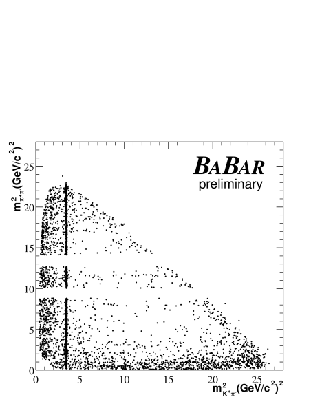
Figure 2 shows the Dalitz plot for on-resonance data within the signal region $5.2715<m_{\rm ES}<5.2865$ ${\rm GeV}/c^{2}$ after cutting on a likelihood ratio formed from the $\Delta E$ and ${\cal F}$ PDFs to enhance the signal over background ratio.

Figure 2: Dalitz plot for on-resonance data within the signal region $5.2715<m_{\rm ES}<5.2865$ ${\rm GeV}/c^{2}$ after cutting on a likelihood ratio formed from the $\Delta E$ and ${\cal F}$ PDFs to enhance the signal over background ratio

4.2.2 Branching fraction measurement

One distinguishes two categories of modes:

• modes which do not suffer from cross-feed with other modes, like in regions III ($\overline{D}^{0}\pi^{+}$) and VIII ($\chi_{c0}K^{+}$). In this case, their branching ratios are simply obtained by:

  $${\cal B}=\frac{Y}{N_{B\bar{B}}\epsilon},$$ (7)

  where $Y$ is the signal yield measured in the previous stage, $N_{B\bar{B}}=(61.6\pm 6.8)\times 10^{6}$ is the number of $B\bar{B}$ pairs, and $\epsilon$ is the reconstruction efficiency calculated using signal Monte Carlo events and corrected to account for data/Monte Carlo discrepancies in tracking and particle identification.

• for the other modes suffering from cross-talk, one uses:

  $${\cal B}=M^{-1}Y/N_{B\bar{B}},$$ (8)

  where ${\cal B}$ and $Y$ are now branching ratio and yield vectors, and $M$ is a matrix representing the probability of an event of a particular mode to be found in a given region. The branching fractions depend on the resonance model assumed in calculating the matrix M, which is split into two component matrices, $P$ and $\epsilon$, such that $M_{ij}=P_{ij}\epsilon_{ij}$. The $P$ matrix accounts for the event distribution within the Dalitz plot, and $\epsilon$ for the reconstruction efficiencies. One assumes one dominant resonance per region, as indicated in the second column of table 1. For regions II, VI and VII, many contributions are possible: the model chosen here respectively includes $K_{0}^{*0}(1430)$, $f_{2}(1270)$ and a flat non-resonant $K^{+}\pi^{-}\pi^{+}$. The masses and widths are taken from the PDG[8], and resonances are modelled by a Breit-Wigner, except for the $\rho(770)$ where the Blatt-Weisskopf parameterization is used[9]. This model suffers from large uncertainties: the dominant resonance is unknown is some regions, there are uncertainties on the masses and widths of the resonances and on the choice of lineshapes. Alternative resonances and lineshapes are used for systematic studies. Possible interferences between resonances are also considered for systematics.

The obtained branching fractions are given in table 2. The systematic errors include components from the measurement itself (tracking efficiencies, particle identification, Fisher PDF, number of $B\bar{B}$ pairs), from the model (resonances contributions, masses, widths and lineshapes) and from the possible interferences (computed by allowing each contribution to have a random phase). These two last sources of systematics are dominant over the first one, except for the $B^{+}\to\overline{D}^{0}\pi^{+}$ mode where only the first source is present. Significant signals are observed in the $B^{+}\to K^{*0}(892)\pi^{+}$, $B^{+}\to f_{0}(980)K^{+}$, $B^{+}\to\chi_{c0}K^{+}$, $B^{+}\to\overline{D}^{0}\pi^{+}$ and $B^{+}\to{\rm higher}~{}K^{*0}\pi^{+}$ channels

4.3 Branching ratios of $B^{+}\to\rho^{0}\rho^{+}$ and $B^{+}\to\rho^{0}K^{*+}$

The first decay described here, $B^{+}\to\rho^{0}\rho^{+}$, enters the isospin analysis of the $B\to\rho\rho$ modes which aims at measuring the angle $\alpha$ of the unitarity triangle. The second decay, $B^{+}\to\rho^{0}K^{*+}$, is expected to be dominated by $b\to s$ loops where physics beyond the Standard Model could enter.

These two decays are reconstructed in the following sub-decays: $K^{*+}\to K^{+}\pi^{0}$, $K^{0}(\to K^{0}_{S}(\to\pi^{+}\pi^{-}))\pi^{+}$, $\rho^{+}\to\pi^{+}\pi^{0}$ and $\rho^{0}\to\pi^{+}\pi^{-}$. Charged tracks are reconstructed using the same criteria than in section 4.1, except for the $K^{0}_{S}$ candidates to allow for a displaced vertex. The $K^{0}_{S}$ candidates must satisfy $|m(\pi^{+}\pi^{-})-m(K^{0})|<12$ ${\rm MeV}/c^{2}$, with the cosine of the angle between their reconstructed flight and momentum directions greater than $0.995$, and the measured proper decay time greater than five times its uncertainty. Photons with a minimum energy of $30$ MeV are paired to form $\pi^{0}$’s, with a typical invariant mass resolution of $7$ ${\rm MeV}/c^{2}$. One therefore selects $\pi^{0}$ by applying a $\pm 15$ ${\rm MeV}/c^{2}$ interval around the nominal $\pi^{0}$ mass. The $K^{*}$ and $\rho$ resonances are formed by pairing two particles which invariant masses are within the following intervals: $0.75<m(K\pi)<1.05$ ${\rm GeV}/c^{2}$ for the $K^{*}$ and $0.52<m(\pi\pi)<1.00$ ${\rm GeV}/c^{2}$ for the $\rho$. To suppress combinatorial background, one cuts at $-0.5$ on the helicity angle, defined as the angle between the direction of one of the two daughters ($K$ for $K^{*}$ and $\pi^{+}$ for $\rho$) and the parent $B$ direction in the resonance rest frame.

$B$ mesons are kinematically isolated by requiring $m_{\rm ES}>5.2$ ${\rm GeV}/c^{2}$ and $|\Delta E|<0.2$ GeV. The continuum background is rejected by cutting on $|{\rm cos}\theta(T_{B},z)|<0.8$. A Fisher discriminant is also constructed (and used in the final likelihood fit) based on the nine cones of the CLEO Fisher, and the additional variables ${\rm cos}\theta(T_{B},z)$ and the cosine of the polar angle between the $B$ momentum and the beam axis.

Charmed $B$ background coming from $D\to K\pi,K\pi\pi$ is vetoed. The remaining small $B$ background is accounted for in the fit.

The final result is extracted using a maximum likelihood fit. The selection efficiencies for transverse and longitudinal angular polarization are averaged and are assigned a systematic error defined by the RMS of a uniform efficiency between the extreme cases ($9\%$ for $\rho^{0}K^{*+}_{K^{0}\pi^{+}}$, $19\%$ for $\rho^{0}K^{*+}_{K^{+}\pi^{0}}$, $18\%$ for $\rho^{0}\rho^{+}$). The branching fractions are given in table 2  Significant signals (above $4\sigma$) are observed in both channels.

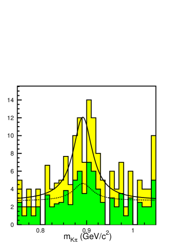
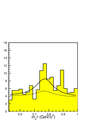
Projections plots of the invariant masses of $K\pi$ for the $B^{+}\to\rho^{0}K^{*+}$ decay, and $\pi^{+}\pi^{-}$ for the $B^{+}\to\rho^{0}\rho^{+}$ decay, are shown in Figure 3.

Figure 3: Projections onto the invariant masses of $K\pi$ (left plot) for the $B^{+}\to\rho^{0}K^{*+}$ decay, and of $\pi^{+}\pi^{-}$ (right plot) for the $B^{+}\to\rho^{0}\rho^{+}$ decay. The histograms show the data (for the $K^{*}$ projection, the shaded area shows the $K^{+}\pi^{0}$ final state only), and the solid (resp. dashed) line shows the signal-plus-background (resp. background only) PDF projections.

5 Gluonic penguins

5.1 Branching fractions, longitudinal components, and direct $CP$ asymmetries in $B\to\phi K^{*}$

The decays $B\to\phi K^{*}$ are expected to proceed through pure $b\to s$ loops, where new physics could enter. Therefore, the measurement of direct $CP$ violation, as well as the measurement of $\sin 2\beta$ via the time-dependent analysis of $B^{0}\to\phi K^{*0}$[2], can probe physics beyond the Standard Model. The analysis of angular distributions in these vector-vector final states is also of interest since information about the decay dynamics can be obtained[11].

The analysis proceeds in a very similar way than what is described in section 4.3, with the additional feature that longitudinal components and direct $CP$ asymmetries are measured in the final likelihood fit. Due to limited statistics, the angular analysis is simplified, and only the longitudinal components $f_{L}=\Gamma_{L}/\Gamma$ are obtained using two-helicity angle distributions:

$$\frac{1}{\Gamma}\frac{d^{2}\Gamma}{d\cos\theta_{1}d\cos\theta_{2}}=\frac{9}{4}\left(\frac{1}{4}(1-f_{L})\sin^{2}\theta_{1}\sin^{2}\theta_{2}+f_{L}\cos^{2}\theta_{1}\cos^{2}\theta_{2}\right),$$ (9)

where $\theta_{1}$ and $\theta_{2}$ are respectively the helicity angles of the $K^{*}$ and the $\phi$.

The results are summarized in table 2. Significant signals ($>10\sigma$) are observed in both channels. Both direct $CP$ asymmetries are compatible with zero.

Figure 4: Projections onto $m_{\rm ES}$ for $B^{0}\to\phi K^{*0}$ (left plot) and $B^{+}\to\phi K^{*+}$ (right plot). The histograms show the data (the shaded area shows the $K^{+}\pi^{0}$ final state only), and the solid (resp. dashed) line shows the signal-plus-background (resp. background only) PDF projections.

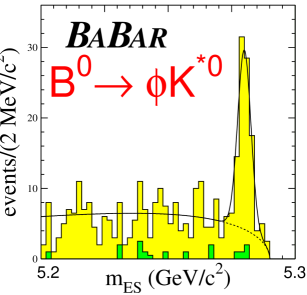
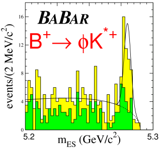
Projections onto $m_{\rm ES}$ of both signals are shown in figure 4.

6 Conclusions

Table 2: Results for the measurements summarized in this proceeding. The first error quoted is statistical and the second error corresponds to systematics. Upper limits are quoted at $90\%$ CL.

Mode	BF ($10^{-6}$)	$A_{\rm CP}$	$\cal L$ ($fb^{-1}$)
Charmless $B$ decays
Inclusive $B^{+}\to h^{+}h^{-}h^{+}$ ($h=\pi,K$) (sec. 4.1)
$B^{+}\to\pi^{+}\pi^{-}\pi^{+}$	$10.9\pm 3.3\pm 1.6$	$-0.39\pm 0.33\pm 0.12$	81.9
$B^{+}\to K^{+}\pi^{-}\pi^{+}$	$59.1\pm 3.8\pm 3.2$	$\phantom{1}0.01\pm 0.07\pm 0.03$	81.9
$B^{+}\to K^{+}K^{-}K^{+}$	$29.6\pm 2.1\pm 1.6$	$\phantom{1}0.02\pm 0.07\pm 0.03$	81.9
$B^{+}\to K^{+}K^{-}\pi^{+}$	$<6.3$	-	81.9
$B^{+}\to K^{-}\pi^{+}\pi^{+}$	$<1.8$	-	81.9
$B^{+}\to K^{+}K^{+}\pi^{-}$	$<1.3$	-	81.9
Exclusive $B^{+}\to K^{+}\pi^{-}\pi^{+}$ (sec. 4.2)
$B^{+}\to K^{*0}(892)\pi^{+}$	$10.3\pm 1.2~{}^{+1.0}_{-2.7}$	-	56.4
$B^{+}\to f_{0}(980)K^{+}$	$9.2\pm 1.2~{}^{+2.1}_{-2.6}$	-	56.4
$B^{+}\to\chi_{c0}K^{+}$	$1.46\pm 0.35\pm 0.12$	-	56.4
$B^{+}\to\overline{D}^{0}\pi^{+}$	$184.6\pm 3.2\pm 9.7$	-	56.4
$B^{+}\to{\rm higher}~{}K^{*0}\pi^{+}$	$25.1\pm 2.0~{}^{+11.0}_{-5.7}$	-	56.4
$B^{+}\to\rho^{0}(770)K^{+}$	$<6.2$	-	56.4
$B^{+}\to K^{+}\pi^{-}\pi^{+}$	$<17.0$	-	56.4
$B^{+}\to{\rm higher~{}}fK^{+}$	$<12.0$	-	56.4
$B^{+}\to\rho^{0}\rho^{+}$ and $B^{+}\to\rho^{0}K^{*+}$ (sec. 4.3)
$B^{+}\to\rho^{0}\rho^{+}$	$9.9^{+2.6}_{-2.5}\pm 1.1$	-	81.9
$B^{+}\to\rho^{0}K^{*+}$	$7.7^{+2.1}_{-2.0}\pm 1.4$	-	81.9
Gluonic penguins
$B\to\phi K^{*}$ (sec. 5.1)
$B^{0}\to\phi K^{*0}$	$11.1^{+1.3}_{-1.2}\pm 1.1$	$+0.04\pm 0.12\pm 0.02$	81.9
	$\Gamma_{L}/\Gamma$ = $0.65\pm 0.07\pm 0.04$
$B^{+}\to\phi K^{*+}$	$12.1^{+2.1}_{-1.9}\pm 1.5$	$+0.16\pm 0.17\pm 0.04$	81.9
	$\Gamma_{L}/\Gamma$ = $0.46\pm 0.12\pm 0.05$

All results presented in these proceedings are summarized in table 2. Many new channels are observed with a large statistical significance. Measurements of direct $CP$ violation do not indicate any significant deviation from zero. A first angular analysis is performed on the vector vector final states $B\to\phi K^{*}$: one measures a large longitudinal component, which should simplify the time dependent analysis allowing to measure $\sin 2\beta$ in $B^{0}\to\phi K^{*0}$. These results, and many others, should become extremely precise as the integrated luminosity will reach $500fb^{-1}$ in the year 2005, and more than $1~{}ab^{-1}$ at the end of the decade.

References

- [1] B. Aubert et al., BABAR Collaboration, Nucl. Instrum. Methods A 479, 1 (2002)
- [2] R. Faccini, these proceedings.
- [3] R.A. Fisher, Annals of Eugenics, 179 (1936)
- [4] A. Snyder and H. Quinn, Phys. Rev. D 48, 2139 (1993)
- [5] D.M. Asner et al., CLEO Collaboration, Phys. Rev. D 53, 1039 (1996)
- [6] N.G. Deshpande, G. Eilam, X.G. He, J. Trampetic, Phys. Rev. D 52, 5354 (1995)
- [7] S. Fajfer, R.J. Oakes, T.N.Pham, Phys. Lett. B 539, 67 (2002)
- [8] Particle Data Group, Phys. Rev. D 66, 01001 (2002)
- [9] J.M. Blatt and V.F. Weisskopf, Theoretical Nuclear Physics (Wiley, New York, 1952) 361
- [10] B. Aubert et al., BABAR Collaboration, hep-ex/0307026
- [11] G. Kramer, W.F Palmer, Phys. Rev. D 45, 193 (1992); C.H. Chen, Y.Y. Keum, H.N. Li, Phys. Rev. D 66, 054013 (2002)