Study of the decay mode $D^{0}\rightarrow K^{-}K^{-}K^{+}\pi^{+}$

Abstract

Using data from the FOCUS (E831) experiment at Fermilab, we present a new measurement of the branching ratio for the Cabibbo-favored decay mode $D^{0}\rightarrow K^{-}K^{-}K^{+}\pi^{+}$.

From a sample of $143\pm 19$ fully reconstructed $D^{0}\to K^{-}K^{-}K^{+}\pi^{+}$ events, we measure $\Gamma(D^{0}\to K^{-}K^{-}K^{+}\pi^{+})/\Gamma(D^{0}\to K^{-}\pi^{-}\pi^{+}\pi^{+})=0.00257\pm 0.00034(stat.)\pm 0.00024(syst.)$.

A coherent amplitude analysis has been performed to determine the resonant substructure of this decay mode. This analysis reveals a dominant contribution from $\phi$ and $\overline{K}^{*0}(892)$ states.

FOCUS Collaboration

1. Introduction

Hadronic decays of charm mesons have been extensively studied in recent years. Dalitz plot analyses of $D$ meson decays in three-body final states have revealed a rich resonant substructure, showing a dominance of quasi two-body modes. However, much less information is available on the resonant substructure of decays with more than three final state particles. These multi-body $D$ decays account for a large fraction of the hadronic decay width. If the amplitude analyses of multi-body decays confirm the picture drawn by the Dalitz plot analyses, then one can make a more complete comparison with theoretical models, which have been developed mainly to describe the two-body and quasi-two-body decay modes [1, 2, 3, 4, 5].

We present a new study of the $D^{0}\to K^{-}K^{-}K^{+}\pi^{+}$ decay using data from the FOCUS experiment. This is an interesting decay mode: although Cabibbo favored, it is strongly suppressed by phase-space and requires the production of an $s\overline{s}$ pair, either from the vacuum or via final state interactions (FSI). We measure the branching ratio ${\frac{{\Gamma(D^{0}\to K^{-}K^{-}K^{+}\pi^{+})}}{{\Gamma(D^{0}\to K^{-}\pi^{-}\pi^{+}\pi^{+})}}}$ and perform a coherent amplitude analysis to determine its resonant substructure.

FOCUS is a charm photoproduction experiment [6] which collected data during the 1996–97 fixed-target run at Fermilab. Electron and positron beams (with typically $300~{}\textrm{GeV}$ endpoint energy) obtained from the $800~{}\textrm{GeV/$c$}$ Tevatron proton beam produce, by means of bremsstrahlung, a photon beam which interacts with a segmented BeO target. The mean photon energy for triggered events is $\sim 180~{}\textrm{GeV}$. A system of three multicell threshold Čerenkov counters performs the charged particle identification, separating kaons from pions with momenta up to $60~{}\textrm{GeV}/c$. Two systems of silicon microvertex detectors are used to track particles: the first system consists of 4 planes of microstrips interleaved with the experimental target [7]; the second system consists of 12 planes of microstrips located downstream of the target. These detectors provide high resolution in the transverse plane (approximately $9~{}\mu\textrm{m}$), allowing the identification and separation of charm primary (production) and secondary (decay) vertices. The charged particle momenta are determined by measuring their deflections in two magnets of opposite polarity through five stations of multiwire proportional chambers.

2. Analysis of the decay mode $D^{0}\to K^{-}K^{-}K^{+}\pi^{+}$

The final states are selected using a candidate driven vertex algorithm [6]. A secondary vertex is formed from the four candidate tracks. The momentum of the resultant $D^{0}$ candidate is used as a seed track to intersect the other reconstructed tracks to search for a primary vertex. The confidence levels of both vertices are required to be greater than $1\%$. Once the production and decay vertices are determined, the distance $\ell$ between them and its error $\sigma_{\ell}$ are computed. The quantity $\ell/\sigma_{\ell}$ is an unbiased measure of the significance of detachment between the primary and secondary vertices. This is the most important variable for separating charm events from non-charm, prompt backgrounds. Signal quality is further enhanced by cutting on Iso2, which is the confidence level that other tracks in the event might be associated with the secondary vertex. To minimize systematic errors on the measurements of the branching ratio, we use identical vertex cuts on the signal and normalizing mode, namely $\ell/\sigma_{\ell}$ $>$ $6$, and Iso2 $<$ 1 $\%$. We also require the $D^{0}$ momentum to be in the range 25–250 GeV/$c$ (a very loose cut) and the primary vertex to be formed with at least two reconstructed tracks in addition to the $D^{0}$ seed.

The only difference in the selection criteria between the two decay modes lies in the particle identification cuts. The Čerenkov identification cuts used in FOCUS are based on likelihood ratios between the various particle identification hypotheses. These likelihoods are computed for a given track from the observed firing response (on or off) of all cells within the track’s ($\beta=1$) Čerenkov cone for each of our three Čerenkov counters. The product of all firing probabilities for all the cells within the three Čerenkov cones produces a $\chi^{2}$-like variable $W_{i}=-2\ln(\mathrm{Likelihood})$ where $i$ ranges over the electron, pion, kaon and proton hypotheses [8]. All kaon tracks are required to have $\Delta_{K}=W_{\pi}-W_{K}$ (kaonicity) greater than $2$, whereas the pion tracks are required to have $\Delta_{\pi}=W_{K}-W_{\pi}$ (pionicity) exceeding $0.5$.

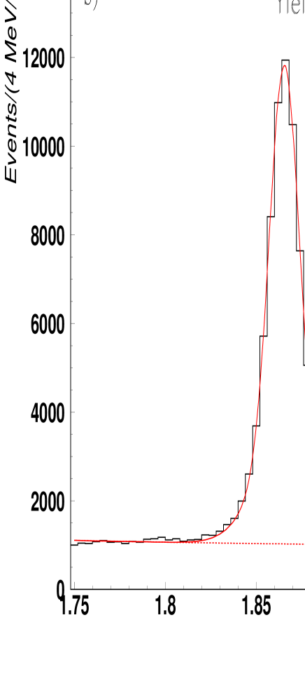
Figure 1: Invariant mass distribution for $K^{-}K^{-}K^{+}\pi^{+}$(a) and $K^{-}\pi^{-}\pi^{+}\pi^{+}$(b). The fit (solid curve) is to two Gaussians for the signal plus a quadratic polynomial for the background.

Using the set of selection cuts just described, we obtain the invariant mass distributions for $K^{-}K^{-}K^{+}\pi^{-}$ and $K^{-}\pi^{-}\pi^{+}\pi^{+}$ shown in Fig. 1. In Fig. 1a the $K^{-}K^{-}K^{+}\pi^{-}$ mass plot is fit with two Gaussians with the same mean but different sigmas to take into account the change in resolution with momentum of our spectrometer [6] plus a second-order polynomial. A log-likelihood fit returns a signal of $143\pm 19$ $D^{0}\to K^{-}K^{-}K^{+}\pi^{-}$ events. The large statistics $K^{-}\pi^{-}\pi^{+}\pi^{+}$ mass plot of Fig. 1b is fitted in the same way (two Gaussians plus a second-order polynomial). The fit gives a signal of $64576\pm 360$ $D^{0}\to K^{-}\pi^{-}\pi^{+}\pi^{+}$ events.

3. Relative Branching Ratio

The evaluation of relative branching ratios requires yields from the fits to be corrected for detection efficiencies, which differ among the various decay modes due to differences in both spectrometer acceptance (due to different $Q$ values and resonant substructure of the two decay modes) and Čerenkov identification efficiency.

From Monte Carlo simulations, we compute the relative efficiency to be: ${\frac{\epsilon(D^{0}\to K^{-}K^{-}K^{+}\pi^{+})}{\epsilon(D^{0}\to K^{-}\pi^{-}\pi^{+}\pi^{+})}}=0.862\pm 0.010$. Combined with the yields measured above we find a branching ratio of $\frac{\Gamma(D^{0}\to K^{-}K^{-}K^{+}\pi^{+})}{\Gamma(D^{0}\to K^{-}\pi^{-}\pi^{+}\pi^{+})}=0.00257\pm 0.00034$.

Our final measurement has been tested by modifying each of the vertex and Čerenkov cuts individually. The branching ratio is stable versus several sets of cuts as shown in Fig. 2 (we vary the confidence level of the secondary vertex from $1\%$ to $10\%$, Iso2 from $10^{-6}$ to $1$, $\ell/\sigma_{\ell}$ from $5$ to $15$, $\Delta_{K}$ from $0.5$ to $4.5$ and finally $\Delta_{\pi}$ from $0.5$ to $4.5$).

Systematic uncertainties on branching ratio measurements can come from different sources. We determine four independent contributions to the systematic uncertainty: the split sample component, the fit variant component, the component due to the particular choice of the vertex and Čerenkov cuts (discussed previously), and the limited statistics of the Monte Carlo.

The split sample component takes into account the systematics introduced by a residual difference between data and Monte Carlo, due to either a possible mismatch in the reproduction of the $D^{0}$ momentum or the change in the experimental conditions of the spectrometer during data collection. This component has been determined by splitting data into four independent sub-samples, according to the $D^{0}$ momentum range (high and low momentum) and the configuration of the vertex detector, that is, before and after the insertion of an upstream silicon system[7]. A technique employed in FOCUS and in the predecessor experiment E687, modeled after the S-factor method from the Particle Data Group [9], is used to try to separate true systematic variations from statistical fluctuations. The branching ratio is evaluated for each of the 4 statistically independent sub-samples and a scaled variance is calculated $\tilde{\sigma}$ (the errors are boosted when $\chi^{2}/(N-1)>1$). The split sample variance $\sigma_{split}$ is defined as the difference between the reported statistical variance and the scaled variance, if the scaled variance exceeds the statistical variance [10].

Another possible source of systematic uncertainty is the fit variant. This component is computed by varying, in a reasonable manner, the fitting conditions on the whole data set. In our study we fixed the widths of the Gaussians to the values obtained by the Monte Carlo simulation, changed the background parametrization (varying the degree of the polynomial), and used one Gaussian instead of two. In addition we considered the variation of the computed efficiency, both for $D^{0}\to K^{-}K^{-}K^{+}\pi^{-}$ and the normalizing decay mode, due to the different resonant substructure simulated in the Monte Carlo. The BR values obtained by these variants are all a priori likely; therefore this uncertainty can be estimated by the rms of the measurements [10].

Analogous to the fit variant, the cut component is estimated using the standard deviation of the values obtained from the many sets of cuts shown in Fig. 2. Actually this is an overestimate of this component because the event samples of the various cut sets are different.

Finally, there is a contribution due to the limited statistics of the Monte Carlo simulation used to determine the efficiencies. The resulting systematic errors are summarized in Table 1. Adding in quadrature the four components, we obtain the total systematic error also shown in Table 1.

Source	Percent
Split sample	$0.0\%$
Fit Variant	$4.1\%$
Set of cuts	$8.3\%$
MC statistics	$1.2\%$
Total systematic	$9.4\%$

Table 1: Contribution in percent to the systematic uncertainties of the branching ratio $\Gamma(D^{0}\to K^{-}K^{-}K^{+}\pi^{+})/\Gamma(D^{0}\to K^{-}\pi^{-}\pi^{+}\pi^{+})$.

The final branching ratio result is shown in Table 2 along with a comparison to previous measurements.

Experiment	$\frac{\Gamma(D^{0}\to K^{-}K^{-}K^{+}\pi^{+})}{\Gamma(D^{0}\to K^{-}\pi^{-}\pi^{+}\pi^{+})}$	Events
E687 [11]	$0.0028\pm 0.0007\pm 0.0001$	$20\pm 5$
E791 [12]	$0.0054\pm 0.0016\pm 0.0008$	$18.4\pm 5.3$
FOCUS (this result)	$0.00257\pm 0.00034\pm 0.00024$	$143\pm 19$

Table 2: Branching ratio measurement and comparison with other experiments.

4. Amplitude analysis of $D^{0}\to K^{-}K^{-}K^{+}\pi^{+}$

A fully coherent amplitude analysis was performed to determine the resonant substructure of the $D^{0}\to K^{-}K^{-}K^{+}\pi^{+}$ decay. While a large number of intermediate states could lead to the $K^{-}K^{-}K^{+}\pi^{+}$ final state, phase space limitations restrict the possible contributions. A plot of the $K^{-}K^{+}$ invariant mass shows a clear $\phi$ contribution (Fig. 3, top left plot). It is also possible, in principle, to have $K^{-}K^{+}$ contribution via $f_{0}(980)$ and $a_{0}(980)$. There are large uncertainties in the line shape of these resonances and in their coupling to $K^{-}K^{+}$. They do not appear to be required by the fit and are therefore not included.

Contributions from $\kappa(800)K^{-}K^{+}$ and $\overline{K}^{*0}(1430)K^{-}K^{+}$ might also be present. However, these resonances are broad scalar states, with no characteristic angular distribution that could distinguish them from the non-resonant mode, with the present level of statistics.

Modes containing a $\overline{K}^{*0}(892)$ can also contribute, even though the nominal  $\overline{K}^{*0}(892)$ mass is just above the kinematical limit of the $K^{-}\pi^{+}$ spectrum. Since $\overline{K}^{*0}(892)$ is a narrow vector meson, its contribution can be distinguished by the angular distribution of the decay products, even without a clear mass peak.

We consider four decay amplitudes: non-resonant, $\phi\overline{K}^{*0}(892)$, $\phi K^{-}\pi^{+}$ and $\overline{K}^{*0}(892)K^{-}K^{+}$. In our default model, model A, we use all four amplitudes. We also consider a simpler model, model B, which does not include the two $\overline{K}^{*0}(892)$ amplitudes.

The formalism used in this amplitude analysis is a straightforward extension to four-body decays of the usual Dalitz plot fit technique. The $D^{0}$ is a spin zero particle, so the four-body decay kinematics are defined by five degrees of freedom.

Individual amplitudes, $A_{k}$, for each resonant mode are constructed as a product of form factors, relativistic Breit-Wigner functions, and spin amplitudes which account for angular momentum conservation. We use the Blatt-Weisskopf damping factors [14], $F_{l}$, as form factors ($l$ is the orbital angular momentum of the decay vertex). For the spin amplitudes we use the Lorentz invariant amplitudes [13], which depend both on the spin of the resonance(s) and the orbital angular momentum. The relativistic Breit-Wigner is

$$BW={1\over{m^{2}-m_{0}^{2}+im_{0}\Gamma(m)}},$$

where

$$\Gamma(m)=\Gamma_{0}\frac{m_{0}}{m}\left(\frac{p^{*}}{p^{*}_{0}}\right)^{2s+1}\frac{F_{s}^{2}}{F_{s0}^{2}}.$$

In the above equations $m$ is the two-body invariant mass, $m_{0}$ and $s$ are the resonance nominal mass and spin, and $p^{*}=p^{*}(m)$ is the breakup momentum at resonance mass $m$.

Since there are two identical kaons, each amplitude $A_{k}$ is Bose-symmetrized. The overall signal amplitude is a coherent sum of the individual amplitudes, $A=\sum_{k}c_{k}A_{k}$, assuming a constant complex amplitude for the non-resonant mode. The coefficients $c_{k}$ are complex numbers to be determined by the fit. The overall signal amplitude is corrected on an event-by-event basis for the acceptance, which is nearly constant across the phase space.

In the amplitude analysis we have taken events having a $K^{-}K^{-}K^{+}\pi^{+}$ invariant mass within the interval $M_{D}\pm 10$ MeV/$c^{2}$. In this interval there are 139 signal and 65 background events. The finite detector resolution causes a smearing of the edges of the five-dimensional phase space. This effect is accounted for by multiplying the overall signal distribution by a Gaussian factor, $g(M)$, where $M$ is the $K^{-}K^{+}K^{-}\pi^{+}$ mass. The normalized signal probability distribution is

$$P_{S}(\phi)=\frac{1}{N_{S}}\varepsilon(\phi)\rho(\phi)g(M)\mid\sum c_{k}A_{k}(\phi)\mid^{2},$$

where $\phi$ represents the coordinates of an event in the five dimensional phase space, $\varepsilon(\phi)$ is the acceptance function, and $\rho(\phi)$ is the phase space density.

Two types of background events were considered: random $\phi$’s combined with a $K^{-}\pi^{+}$ pair, and random combinations of $K^{-}K^{-}K^{+}\pi^{+}$. Inspection of the side bands of the $K^{-}K^{-}K^{+}\pi^{+}$ mass spectrum indicate that nearly 30% of the background events are of the former type. We assume the random $K^{-}K^{-}K^{+}\pi^{+}$ combinations to be uniformly distributed in phase space, while for the $\phi$ background we assume an incoherent sum of Breit-Wigners with no form factors and no angular distribution. The overall background distribution, kept fixed in the fit, is a weighted, incoherent sum of these two components. The overall background distribution is also corrected for the acceptance (assumed to be the same as for the signal events) on an event-by-event basis, and multiplied by an exponential function $b(M)$, to account for the detector resolution. The normalized background probability distribution is

$$P_{B}(\phi)=\frac{1}{N_{B}}\varepsilon(\phi)\rho(\phi)b(M)\sum b_{k}B_{k}(\phi).$$

An unbinned maximum likelihood fit was performed, minimizing the quantity $w\equiv-2\ln{\mathcal{L}}$. The likelihood function, $\mathcal{L}$, is

$$\mathcal{L}=\prod_{events}\left[P_{S}(\phi^{i})+P_{B}(\phi^{i})\right]$$

Neither the acceptance function nor the phase space density depend on the fit parameters $c_{k}$, so the term $-2ln\left[\varepsilon(\phi)\rho(\phi)\right]$ is irrelevant to the minimization. The acceptance correction is important only for the normalization integrals $N_{S}$ and $N_{B}$.

Decay fractions are obtained from the coefficients $c_{k}$ determined by the fit, after integrating the overall signal amplitude over the phase space:

$$f_{k}=\frac{\int d\phi\mid c_{k}A_{k}\mid^{2}}{\int d\phi\mid\sum_{j}c_{j}A_{j}\mid^{2}}.$$

We fit the data to both models A and B. We find that model B, with only the non-resonant and $\phi K^{-}\pi^{+}$ contributions, does not provide a good description of the data. The inclusion of the two $\overline{K}^{*0}(892)$ amplitudes results in a much better fit, with an improvement in $\Delta w$ of 138.

Results from the fit with model A are shown in Table 3. The dominant contribution comes from $D^{0}\to\phi\overline{K}^{*0}(892)$. Adding the contributions from the two $\overline{K}^{*0}(892)$ amplitudes, we see that they account for nearly $70\%$ of the total decay width. This is somewhat surprising, given the very small phase space. In Fig. 3 the $K^{+}K^{-}$ and $K^{-}\pi^{+}$ projections of events used in the amplitude analysis are superimposed on the fit result (top two plots). The projections from the background model are shown in the shaded histograms. The remaining plots are two-dimensional projections of the events in the signal region.

We have performed a log-likelihood test to check our ability to distinguish between models A and B. Two ensembles of 10,000 mini-MC samples were generated, one simulated according to model A and another according to model B. For each sample in each ensemble we compute the quantity $\Delta w=2\ln{\mathcal{L}_{A}}-2\ln{\mathcal{L}_{B}}$, where $\mathcal{L}_{B}$ and $\mathcal{L}_{A}$ are the likelihoods calculated with models B and A, respectively. The resulting $\Delta w$ distributions are shown in Fig. 4. On the right we see the $\Delta w$ distribution computed from the model A ensemble, and, on the left, $\Delta w$ with the model B ensemble. The two distributions are well separated showing that we can easily distinguish between these two models. Moreover, the value of $\Delta w$ obtained from the real data (138) is consistent with the distribution from model A, showing that this is indeed a better description of the data.

The goodness-of-fit was assessed in two ways. We have estimated the confidence level of the fit using a $\chi^{2}$ test. The five invariants used to define the kinematics of this decay are the four $K^{-}K^{+}$ and $K^{-}\pi^{+}$ masses squared, plus either the $K^{-}K^{-}$ or $K^{+}\pi^{+}$ mass squared. Due to the limited statistics we have integrated over the latter invariant and divided the other four into two bins, yielding a total of sixteen cells. A $\chi^{2}$ was computed and the estimated confidence level was 35%. The confidence level obtained with model B was 6$\times$10^-11.

Given the limited statistics we have also estimated the confidence level using a method which is often less stringent than the $\chi^{2}$. In this second method the confidence level is estimated using the distribution of $w=-2\ln{\mathcal{L}}$ from an ensemble of mini-MC samples generated with the parameters of model A. This distribution is approximately Gaussian. A confidence level can be estimated by the fraction of samples in which the value of $w$ exceeds that of the data. With this technique we estimate a CL of 86% for the fit with model A.

As in the branching ratio measurement, we consider split sample and fit variant systematic uncertainties, using for the former the same sub-samples described previously. The dominant contributions from fit variant systematic errors come from variations on the signal amplitudes (removing the Blatt-Weisskopf form factors and replacing the non-resonant amplitude by $\overline{K}^{*0}(1430)K^{+}K^{-}$), variations in the background relative fractions, and variations of the analysis cuts. Split sample and fit variant errors are added in quadrature. Table 3 shows the Model A fit results. The systematic errors are the second errors in the fractions and phases.

mode	magnitude	phase(deg.)	fraction(%)
$\phi\overline{K}^{*0}(892)$	1	0	48 $\pm$ 6 $\pm$ 1
$\phi K^{-}\pi^{+}$	0.60 $\pm$ 0.12	194 $\pm$ 24 $\pm$ 8	18 $\pm$ 6 $\pm$ 4
$\overline{K}^{*0}(892)K^{+}K^{-}$	0.65 $\pm$ 0.13	255 $\pm$ 15 $\pm$ 4	20 $\pm$ 7 $\pm$ 2
non-resonant	0.55 $\pm$ 0.14	278 $\pm$ 16 $\pm$ 42	15 $\pm$ 6 $\pm$ 2

Table 3: Results from the best fit (Model A). The second error on the fractions and phases is systematic.

5. Conclusions

Using data from the FOCUS (E831) experiment at Fermilab, we have studied the Cabibbo-favored decay mode $D^{0}\rightarrow K^{-}K^{-}K^{+}\pi^{+}$.

A comparison with the two previous determinations of the relative branching ratio $\frac{\Gamma(D^{0}\to K^{-}K^{-}K^{+}\pi^{+})}{\Gamma(D^{0}\to K^{-}\pi^{-}\pi^{+}\pi^{+})}$ shows an impressive improvement in the accuracy of this measurement.

A coherent amplitude analysis of the $K^{-}K^{-}K^{+}\pi^{+}$ final state was performed for the first time, showing that the dominant contribution comes from $D^{0}\to\phi\overline{K}^{*0}(892)$. This channel, $D^{0}$ decaying to two vector mesons, corresponds to 50% of the $D^{0}\to K^{-}K^{-}K^{+}\pi^{+}$ decay rate. The $\overline{K}^{*0}(892)$ amplitudes, in spite of the limited phase space, account for nearly 70% of the total decay width. Looking at the $K^{+}K^{-}$ spectrum we see that over 60% comes from $D^{0}\to\phi\overline{K}^{*0}(892)$ and $D^{0}\to\phi K^{-}\pi^{+}$.

We wish to acknowledge the assistance of the staffs of Fermi National Accelerator Laboratory, the INFN of Italy, and the physics departments of the collaborating institutions. This research was supported in part by the U. S. National Science Foundation, the U. S. Department of Energy, the Italian Istituto Nazionale di Fisica Nucleare and Ministero della Istruzione Università e Ricerca, the Brazilian Conselho Nacional de Desenvolvimento Científico e Tecnológico, CONACyT-México, and the Korea Research Foundation of the Korean Ministry of Education.

Figure 2: Branching ratio $\Gamma(D^{0}\to K^{-}K^{-}K^{+}\pi^{+})/\Gamma(D^{0}\to K^{-}\pi^{-}\pi^{+}\pi^{+})$ versus several sets of cuts. From left to right, we vary the confidence level of the secondary vertex from $1\%$ to $10\%$ (10 points), Iso2 from $10^{-6}$ to $1$ (7 points), $L$ / $\sigma_{L}$ from $5$ to $15$ (11 points), $\Delta_{K}$ from $0.5$ to $4.5$ (9 points) and $\Delta_{\pi}$ from $0.5$ to $4.5$ (9 points).

Figure 3: The top two plots are projections of the invariant mass distribution $K^{-}K^{+}$ and $K^{-}\pi^{+}$, with the fit results superimposed (solid histograms). The shaded histograms are the background projections. The left scatter plots show the data population for $K^{-}K^{+}$ and $K^{-}\pi^{+}$ from the signal region, while the right ones show the fit results. Due to two identical particles in the final state, there are two entries per event in each plot.

Figure 4: Distributions of difference in log-likelihood from ensembles of simulated samples generated according to model B (left distribution) and model A (right distribution).

References

- [1] M. Bauer, B. Steck and M. Wirbel, Z. Phys. C34 (1987) 103.
- [2] B.T. Block and M.A. Shifman, Sov. J. Nucl. Phys. 45 (1987) 522.
- [3] F. Buccella et al., Z. Phys. C55 (1992) 243.
- [4] L.L. Chau and H.Y. Cheng, Phys. Rev. D36 (1987) 137.
- [5] P. Bedaque, A. Das, and V.S. Mathur, Phys. Rev. D49 (1994) 269.
- [6] E687 Collaboration, P.L. Frabetti et al., Nucl. Instrum. Meth. A320 (1992) 519.
- [7] FOCUS Collaboration, J.M. Link et al., hep-ex/0204023, submitted to Nucl. Instrum. Meth. A.
- [8] FOCUS Collaboration, J.M. Link et al., Nucl. Instrum. Meth. A484 (2002) 270.
- [9] K. Hagiwara et al. (Particle Data Group), Phys. Rev. D66 (2002) 010001.
- [10] FOCUS Collaboration, J.M. Link et al., Phys. Lett. B555 (2003) 173.
- [11] E687 Collaboration, P.L. Frabetti et al., Phys. Lett. B354 (1995) 486.
- [12] E791 Collaboration, E.M. Aitala et al., Phys. Rev. D64 (2001) 112003.
- [13] MARKIII Collaboration, D. Coffman et al., Phys. Rev. D45 (1992) 2196.
- [14] J.M. Blatt and V.F. Weisskopf, Theoretical Nuclear Physics, page 361, John Wiley & Sons, New York, 1952.