EUROPEAN ORGANIZATION FOR NUCLEAR RESEARCH

CERN-EP/2003-041

July 14, 2003

Search for the Single Production of Doubly-Charged Higgs Bosons and Constraints on their Couplings from Bhabha Scattering

The OPAL Collaboration

A search for the single production of doubly-charged Higgs bosons is performed using ${\rm e^{+}e^{-}}$ collision data collected by the OPAL experiment at centre-of-mass energies between 189 GeV and 209 GeV. No evidence for the existence of ${\rm H}^{\pm\pm}$ is observed. Upper limits are derived on ${\rm h_{ee}}$, the Yukawa coupling of the ${\rm H}^{\pm\pm}$ to like-signed electron pairs. A 95% confidence level upper limit of ${\rm h_{ee}}<$ 0.071 is inferred for $M({\rm H}^{\pm\pm})<$ 160 GeV assuming that the sum of the branching fractions of the ${\rm H}^{\pm\pm}$ to all lepton flavour combinations is 100%. Additionally, indirect constraints on ${\rm h_{ee}}$ from Bhabha scattering at centre-of-mass energies between 183 GeV and 209 GeV, where the ${\rm H}^{\pm\pm}$ would contribute via $t$-channel exchange, are derived for $M({\rm H}^{\pm\pm})<$ 2 TeV. These are the first results both from a single production search and on constraints from Bhabha scattering reported from LEP.

Submitted to Phys.Lett.B

The OPAL Collaboration

G. Abbiendi², C. Ainsley⁵, P.F. Åkesson³, G. Alexander²², J. Allison¹⁶, P. Amaral⁹, G. Anagnostou¹, K.J. Anderson⁹, S. Arcelli², S. Asai²³, D. Axen²⁷, G. Azuelos^18,a, I. Bailey²⁶, E. Barberio^8,p, R.J. Barlow¹⁶, R.J. Batley⁵, P. Bechtle²⁵, T. Behnke²⁵, K.W. Bell²⁰, P.J. Bell¹, G. Bella²², A. Bellerive⁶, G. Benelli⁴, S. Bethke³², O. Biebel³¹, O. Boeriu¹⁰, P. Bock¹¹, M. Boutemeur³¹, S. Braibant⁸, L. Brigliadori², R.M. Brown²⁰, K. Buesser²⁵, H.J. Burckhart⁸, S. Campana⁴, R.K. Carnegie⁶, B. Caron²⁸, A.A. Carter¹³, J.R. Carter⁵, C.Y. Chang¹⁷, D.G. Charlton¹, A. Csilling²⁹, M. Cuffiani², S. Dado²¹, A. De Roeck⁸, E.A. De Wolf^8,s, K. Desch²⁵, B. Dienes³⁰, M. Donkers⁶, J. Dubbert³¹, E. Duchovni²⁴, G. Duckeck³¹, I.P. Duerdoth¹⁶, E. Etzion²², F. Fabbri², L. Feld¹⁰, P. Ferrari⁸, F. Fiedler³¹, I. Fleck¹⁰, M. Ford⁵, A. Frey⁸, A. Fürtjes⁸, P. Gagnon¹², J.W. Gary⁴, G. Gaycken²⁵, C. Geich-Gimbel³, G. Giacomelli², P. Giacomelli², M. Giunta⁴, J. Goldberg²¹, M. Groll²⁵, E. Gross²⁴, J. Grunhaus²², M. Gruwé⁸, P.O. Günther³, A. Gupta⁹, C. Hajdu²⁹, M. Hamann²⁵, G.G. Hanson⁴, K. Harder²⁵, A. Harel²¹, M. Harin-Dirac⁴, M. Hauschild⁸, C.M. Hawkes¹, R. Hawkings⁸, R.J. Hemingway⁶, C. Hensel²⁵, G. Herten¹⁰, R.D. Heuer²⁵, J.C. Hill⁵, K. Hoffman⁹, D. Horváth^29,c, P. Igo-Kemenes¹¹, K. Ishii²³, H. Jeremie¹⁸, P. Jovanovic¹, T.R. Junk⁶, N. Kanaya²⁶, J. Kanzaki^23,u, G. Karapetian¹⁸, D. Karlen²⁶, K. Kawagoe²³, T. Kawamoto²³, R.K. Keeler²⁶, R.G. Kellogg¹⁷, B.W. Kennedy²⁰, D.H. Kim¹⁹, K. Klein^11,t, A. Klier²⁴, S. Kluth³², T. Kobayashi²³, M. Kobel³, S. Komamiya²³, L. Kormos²⁶, T. Krämer²⁵, P. Krieger^6,l, J. von Krogh¹¹, K. Kruger⁸, T. Kuhl²⁵, M. Kupper²⁴, G.D. Lafferty¹⁶, H. Landsman²¹, D. Lanske¹⁴, J.G. Layter⁴, A. Leins³¹, D. Lellouch²⁴, J. Letts^o, L. Levinson²⁴, J. Lillich¹⁰, S.L. Lloyd¹³, F.K. Loebinger¹⁶, J. Lu^27,w, J. Ludwig¹⁰, A. Macpherson^28,i, W. Mader³, S. Marcellini², A.J. Martin¹³, G. Masetti², T. Mashimo²³, P. Mättig^m, W.J. McDonald²⁸, J. McKenna²⁷, T.J. McMahon¹, R.A. McPherson²⁶, F. Meijers⁸, W. Menges²⁵, F.S. Merritt⁹, H. Mes^6,a, A. Michelini², S. Mihara²³, G. Mikenberg²⁴, D.J. Miller¹⁵, S. Moed²¹, W. Mohr¹⁰, T. Mori²³, A. Mutter¹⁰, K. Nagai¹³, I. Nakamura^23,V, H. Nanjo²³, H.A. Neal³³, R. Nisius³², S.W. O’Neale¹, A. Oh⁸, A. Okpara¹¹, M.J. Oreglia⁹, S. Orito^23,∗, C. Pahl³², G. Pásztor^4,g, J.R. Pater¹⁶, G.N. Patrick²⁰, J.E. Pilcher⁹, J. Pinfold²⁸, D.E. Plane⁸, B. Poli², J. Polok⁸, O. Pooth¹⁴, M. Przybycień^8,n, A. Quadt³, K. Rabbertz^8,r, C. Rembser⁸, P. Renkel²⁴, J.M. Roney²⁶, S. Rosati³, Y. Rozen²¹, K. Runge¹⁰, K. Sachs⁶, T. Saeki²³, E.K.G. Sarkisyan^8,j, A.D. Schaile³¹, O. Schaile³¹, P. Scharff-Hansen⁸, J. Schieck³², T. Schörner-Sadenius⁸, M. Schröder⁸, M. Schumacher³, C. Schwick⁸, W.G. Scott²⁰, R. Seuster^14,f, T.G. Shears^8,h, B.C. Shen⁴, P. Sherwood¹⁵, G. Siroli², A. Skuja¹⁷, A.M. Smith⁸, R. Sobie²⁶, S. Söldner-Rembold^16,d, F. Spano⁹, A. Stahl³, K. Stephens¹⁶, D. Strom¹⁹, R. Ströhmer³¹, S. Tarem²¹, M. Tasevsky⁸, R.J. Taylor¹⁵, R. Teuscher⁹, M.A. Thomson⁵, E. Torrence¹⁹, D. Toya²³, P. Tran⁴, I. Trigger⁸, Z. Trócsányi^30,e, E. Tsur²², M.F. Turner-Watson¹, I. Ueda²³, B. Ujvári^30,e, C.F. Vollmer³¹, P. Vannerem¹⁰, R. Vértesi³⁰, M. Verzocchi¹⁷, H. Voss^8,q, J. Vossebeld^8,h, D. Waller⁶, C.P. Ward⁵, D.R. Ward⁵, P.M. Watkins¹, A.T. Watson¹, N.K. Watson¹, P.S. Wells⁸, T. Wengler⁸, N. Wermes³, D. Wetterling¹¹ G.W. Wilson^16,k, J.A. Wilson¹, G. Wolf²⁴, T.R. Wyatt¹⁶, S. Yamashita²³, D. Zer-Zion⁴, L. Zivkovic²⁴

¹School of Physics and Astronomy, University of Birmingham, Birmingham B15 2TT, UK
²Dipartimento di Fisica dell’ Università di Bologna and INFN, I-40126 Bologna, Italy
³Physikalisches Institut, Universität Bonn, D-53115 Bonn, Germany
⁴Department of Physics, University of California, Riverside CA 92521, USA
⁵Cavendish Laboratory, Cambridge CB3 0HE, UK
⁶Ottawa-Carleton Institute for Physics, Department of Physics, Carleton University, Ottawa, Ontario K1S 5B6, Canada
⁸CERN, European Organisation for Nuclear Research, CH-1211 Geneva 23, Switzerland
⁹Enrico Fermi Institute and Department of Physics, University of Chicago, Chicago IL 60637, USA
¹⁰Fakultät für Physik, Albert-Ludwigs-Universität Freiburg, D-79104 Freiburg, Germany
¹¹Physikalisches Institut, Universität Heidelberg, D-69120 Heidelberg, Germany
¹²Indiana University, Department of Physics, Bloomington IN 47405, USA
¹³Queen Mary and Westfield College, University of London, London E1 4NS, UK
¹⁴Technische Hochschule Aachen, III Physikalisches Institut, Sommerfeldstrasse 26-28, D-52056 Aachen, Germany
¹⁵University College London, London WC1E 6BT, UK
¹⁶Department of Physics, Schuster Laboratory, The University, Manchester M13 9PL, UK
¹⁷Department of Physics, University of Maryland, College Park, MD 20742, USA
¹⁸Laboratoire de Physique Nucléaire, Université de Montréal, Montréal, Québec H3C 3J7, Canada
¹⁹University of Oregon, Department of Physics, Eugene OR 97403, USA
²⁰CLRC Rutherford Appleton Laboratory, Chilton, Didcot, Oxfordshire OX11 0QX, UK
²¹Department of Physics, Technion-Israel Institute of Technology, Haifa 32000, Israel
²²Department of Physics and Astronomy, Tel Aviv University, Tel Aviv 69978, Israel
²³International Centre for Elementary Particle Physics and Department of Physics, University of Tokyo, Tokyo 113-0033, and Kobe University, Kobe 657-8501, Japan
²⁴Particle Physics Department, Weizmann Institute of Science, Rehovot 76100, Israel
²⁵Universität Hamburg/DESY, Institut für Experimentalphysik, Notkestrasse 85, D-22607 Hamburg, Germany
²⁶University of Victoria, Department of Physics, P O Box 3055, Victoria BC V8W 3P6, Canada
²⁷University of British Columbia, Department of Physics, Vancouver BC V6T 1Z1, Canada
²⁸University of Alberta, Department of Physics, Edmonton AB T6G 2J1, Canada
²⁹Research Institute for Particle and Nuclear Physics, H-1525 Budapest, P O Box 49, Hungary
³⁰Institute of Nuclear Research, H-4001 Debrecen, P O Box 51, Hungary
³¹Ludwig-Maximilians-Universität München, Sektion Physik, Am Coulombwall 1, D-85748 Garching, Germany
³²Max-Planck-Institute für Physik, Föhringer Ring 6, D-80805 München, Germany
³³Yale University, Department of Physics, New Haven, CT 06520, USA

^a and at TRIUMF, Vancouver, Canada V6T 2A3
^c and Institute of Nuclear Research, Debrecen, Hungary
^d and Heisenberg Fellow
^e and Department of Experimental Physics, Lajos Kossuth University, Debrecen, Hungary
^f and MPI München
^g and Research Institute for Particle and Nuclear Physics, Budapest, Hungary
^h now at University of Liverpool, Dept of Physics, Liverpool L69 3BX, U.K.
ⁱ and CERN, EP Div, 1211 Geneva 23
^j and Manchester University
^k now at University of Kansas, Dept of Physics and Astronomy, Lawrence, KS 66045, U.S.A.
^l now at University of Toronto, Dept of Physics, Toronto, Canada
^m current address Bergische Universität, Wuppertal, Germany
ⁿ now at University of Mining and Metallurgy, Cracow, Poland
^o now at University of California, San Diego, U.S.A.
^p now at Physics Dept Southern Methodist University, Dallas, TX 75275, U.S.A.
^q now at IPHE Université de Lausanne, CH-1015 Lausanne, Switzerland
^r now at IEKP Universität Karlsruhe, Germany
^s now at Universitaire Instelling Antwerpen, Physics Department, B-2610 Antwerpen, Belgium
^t now at RWTH Aachen, Germany
^u and High Energy Accelerator Research Organisation (KEK), Tsukuba, Ibaraki, Japan
^v now at University of Pennsylvania, Philadelphia, Pennsylvania, USA
^w now at TRIUMF, Vancouver, Canada
^∗ Deceased

1 Introduction

Some theories beyond the Standard Model predict the existence of doubly-charged Higgs bosons, ${\rm H}^{\pm\pm}$, including in Left-Right Symmetric models [1], Higgs Triplet models [2], and little Higgs models [3]. It has been particularly emphasized that a see-saw mechanism used to obtain light neutrinos in a model with heavy right-handed neutrinos can lead to a doubly-charged Higgs boson with a mass accessible to current and future colliders [4].

A review of experimental constraints on doubly-charged Higgs bosons is presented in [5]. The pair production of doubly-charged Higgs bosons has been considered in a previous OPAL publication [6], where masses less than 98.5 GeV are excluded for doubly-charged Higgs bosons in Left-Right Symmetric models. DELPHI has obtained a limit of 97.3 GeV, independent of the lifetime of the ${\rm H}^{\pm\pm}$ [7].

It has been noted that doubly-charged Higgs bosons may be singly produced in $\rm e\gamma$ collisions, including in ${\rm e^{+}e^{-}}$ collisions where the $\gamma$ is obtained from radiation from the other beam particle [8, 9]. The diagrams for the direct production are shown in Figure 1.

Figure 1: Feynman diagrams contributing to the single production of $\rm H^{--}$ bosons in ${\rm e^{+}e^{-}}$ collisions. The three additional diagrams with “crossed” $\rm e^{+}$ lines are not shown.

Doubly-charged Higgs bosons would decay into like-signed lepton or vector boson pairs, or to a W boson and a singly-charged Higgs boson. For masses less than twice the W boson mass, they would decay predominantly into like-signed leptons. Furthermore, in most models the WW branching fraction is negligible even for larger masses [9], therefore the dominant decay mode, even for masses larger than twice the W boson mass, is the decay to like-signed leptons. Since the ${\rm H}^{\pm\pm}$ naturally violates lepton number conservation, it can have mixed lepton flavour decay modes. Additionally, the Yukawa coupling of the ${\rm H}^{\pm\pm}$ to the charged leptons h_ℓℓ is model dependent, and is not generally determined directly by the lepton mass, so decays to all lepton flavour combinations need to be considered. It should be particularly noted that mixed lepton flavour decays are severely constrained by rare decay searches such as $\mu^{+}\rightarrow\rm e^{+}e^{+}e^{-}$ and $\mu\rightarrow\rm e\gamma$.

In this paper, we search for the single production of doubly-charged Higgs bosons, assuming the decays ${\rm H}^{\pm\pm}\rightarrow\ell^{\pm}\ell^{\prime\pm}$ using 600.7 pb^-1 of ${\rm e^{+}e^{-}}$ collision data with centre-of-mass energies $\sqrt{s}=$ 189–209 GeV collected by the OPAL detector. Since the production cross-section depends only on ${\rm h_{ee}}$, the Yukawa coupling of the ${\rm H}^{\pm\pm}$ to like-signed electron pairs, the search is sensitive to this quantity.

We assume that the decay of a doubly-charged Higgs boson into a W boson and a singly-charged Higgs boson is negligible. We consider an ${\rm H}^{\pm\pm}$ which couples to right-handed particles, but the results of the direct search quoted here are also valid for an ${\rm H}^{\pm\pm}$ which couples only to left-handed particles [9]. All lepton flavour combinations are considered in the ${\rm H}^{\pm\pm}$ decay ($\rm ee$, $\mu\mu$, $\tau\tau$, $\rm e\mu$, $\rm e\tau$, $\mu\tau$). The lifetime of the ${\rm H}^{\pm\pm}$ can be important, and in particular is non-negligible for ${\rm h_{\ell\ell}}<10^{-7}$; however, our search is not sensitive to such small Yukawa couplings.

A doubly-charged Higgs boson would also affect the Bhabha scattering cross-section via the $t$-channel exchange diagram shown in Figure 2, causing a change in rate and in the observed angular distribution of the outgoing electron. Constraints have been derived for this process using data from lower energy colliders [5], but not previously from LEP.

Figure 2: Feynman diagram contributing to the process ${\rm e^{+}e^{-}}\rightarrow{\rm e^{+}e^{-}}$ due to doubly-charged Higgs boson $t$-channel exchange.

In addition to the direct search results introduced above, we also derive indirect constraints on ${\rm h_{ee}}$, the Yukawa coupling of ${\rm H}^{\pm\pm}$ to electrons, using the differential cross-section of wide-angle Bhabha scattering measured by OPAL in 688.4 pb^-1 of data collected at $\sqrt{s}=$ 183–209 GeV.

2 OPAL Detector

The OPAL detector is described in detail in [10]. It is a multipurpose apparatus with almost complete solid angle coverage. The central detector consists of a silicon micro-strip detector and a system of gas-filled tracking chambers in a 0.435 T solenoidal magnetic field which is parallel to the beam axis. A lead-glass electromagnetic calorimeter with a presampler surrounds the central detector. In combination with the forward calorimeters, the forward scintillating-tile counters, and the silicon-tungsten luminometer, a geometrical acceptance is provided down to 25 mrad from the beam direction. The silicon-tungsten luminometer measures the integrated luminosity using small-angle Bhabha scattering events. The magnet return yoke is instrumented for hadron calorimetry, and is surrounded by several layers of muon chambers.

3 Direct Search

3.1 Data Samples and Event Simulation

The data samples are summarised in Table 1.

$E_{\rm cm}$	$\langle E_{\rm cm}\rangle$	$\int\cal{L}$
(GeV)	(GeV)	($\rm pb^{-1}$)
188 – 190	188.6	175.0
190 – 194	191.6	28.9
194 – 198	195.5	74.8
198 – 201	199.5	78.1
201 – 203	201.7	38.2
203 – 206	205.0	79.4
206 – 209	206.6	126.1
188 – 209	197.7	600.7

Table 1: Data samples used in the direct search analysis.

The process $\rm{\rm e^{+}e^{-}}\rightarrow e^{\mp}e^{\mp}{\rm H}^{\pm\pm}$ is simulated with the PYTHIA6.150 [11] event generator. In the simulation, the Equivalent Photon Approximation (EPA) is used to give an effective flux of photons originating from the electrons or positrons. The upper limit of the virtuality $Q^{2}$ of the photon is given by the scale of the hard scattering process. The process $\rm e^{\pm}\gamma\rightarrow e^{\mp}{\rm H}^{\pm\pm}$ is simulated in a Left-Right Symmetric model for an ${\rm H}^{\pm\pm}$ which couples to right-handed particles using the calculations from [8]. The contribution from ${\rm Z}$-exchange is negligible. In order to obtain the full signal cross-section, a cut which PYTHIA applies by default at a minimum of 1 GeV on the transverse momentum of the lepton which radiates the ${\rm H}^{\pm\pm}$ is explicitly switched off. The cross-section and the angular distribution are checked with the calculations of [9], using COMPHEP [12].

Separate samples are simulated with the 6 different decay modes ($\rm ee$, $\mu\mu$, $\tau\tau$, $\rm e\mu$, $\rm e\tau$, $\mu\tau$). Samples of 500 events each are generated for each of the average centre-of-mass energies listed in Table 1 for ${\rm H}^{\pm\pm}$ masses in 5 GeV steps from 90–200 GeV. For masses larger than twice the W boson mass the decay $\rm{\rm H}^{\pm\pm}\rightarrow W^{\pm}W^{\pm}$ is kinematically allowed. Its partial width, however, is negligible in most models [9]. In this paper, the branching fraction BR($\rm{\rm H}^{\pm\pm}\rightarrow W^{\pm}W^{\pm}$) is assumed to be zero.

The dominant Standard Model backgrounds in this analysis are from the four-fermion processes ${\rm e^{+}e^{-}}\rightarrow\ell^{+}\ell^{-}\ell^{\prime+}\ell^{\prime-}$, including events from the so-called “multi-peripheral” diagrams ${\rm e^{+}e^{-}}\rightarrow{\rm e^{+}e^{-}}\gamma^{(*)}\gamma^{(*)}\rightarrow{\rm e^{+}e^{-}}\ell^{+}\ell^{-}$, and lepton pairs, ${\rm e^{+}e^{-}}\rightarrow\ell^{+}\ell^{-}$. Four-fermion processes except ${\rm e^{+}e^{-}}\rightarrow{\rm e^{+}e^{-}}\ell^{+}\ell^{-}$ ($\ell={\rm e},\mu,\tau$) and ${\rm e^{+}e^{-}}\rightarrow{\rm e^{+}e^{-}}{\rm q\bar{q}}$ are simulated with the KORALW event generator [13]. The non-multi-peripheral part of the processes ${\rm e^{+}e^{-}}\rightarrow{\rm e^{+}e^{-}}\ell^{+}\ell^{-}$ and ${\rm e^{+}e^{-}}\rightarrow{\rm e^{+}e^{-}}{\rm q\bar{q}}$ is simulated with grc4f2.1[14]. The multi-peripheral diagrams are simulated with the dedicated two-photon event generators Vermaseren [15] for ${\rm e^{+}e^{-}}\rightarrow{\rm e^{+}e^{-}}\gamma^{(*)}\gamma^{(*)}\rightarrow{\rm e^{+}e^{-}}{\rm e^{+}e^{-}}$ and BDK [16] for ${\rm e^{+}e^{-}}\rightarrow{\rm e^{+}e^{-}}\gamma^{(*)}\gamma^{(*)}\rightarrow{\rm e^{+}e^{-}}\mu^{+}\mu^{-}$ and ${\rm e^{+}e^{-}}\rightarrow{\rm e^{+}e^{-}}\gamma^{(*)}\gamma^{(*)}\rightarrow{\rm e^{+}e^{-}}\tau^{+}\tau^{-}$. The Monte Carlo generators PHOJET [17] (for $Q^{2}<4.5$ GeV²) and HERWIG [18] (for $Q^{2}\geq 4.5$ GeV²) are used to simulate hadronic events from two-photon processes. Lepton pairs are simulated using the KK2f [19] generator for $\tau^{+}\tau^{-}(\gamma)$ and $\mu^{+}\mu^{-}(\gamma)$ events and NUNUGPV [20] for $\nu\bar{\nu}\gamma(\gamma)$. Bhabha scattering is simulated with BHWIDE [21] (when both the electron and positron scatter at least 12.5^∘ from the beam axis) and TEEGG [22] (for the remaining phase space).

Multihadronic events, ${\rm q\bar{q}}(\gamma)$, are simulated using KK2f [19]. RADCOR [23] is used to simulate multi-photon events from QED processes. They make a negligible contribution to the background.

Generated signal and background events are processed through the full simulation of the OPAL detector [24] and the same event analysis chain was applied to the simulated events as to the data.

3.2 Analysis

The signal final state consists of four charged leptons. Two like-sign leptons originate from the ${\rm H}^{\pm\pm}$ decay and are expected to be visible in the detector in most cases. The electron or positron which originates from the ee$\gamma$ vertex (see Fig. 1) in general escapes through the beampipe. The electron or positron which originates from the ee${\rm H}^{\pm\pm}$ vertex is also forward peaked; however, it enters the detector in a significant fraction of signal events. The analysis is therefore divided into a two-lepton and a three-lepton analysis. The final states in the three-lepton case contain three leptons visible in the detector, two of them have the same sign and could originate from the decay of a doubly-charged Higgs boson. In the two-lepton case, two like-signed leptons are required, as expected in the decay of a doubly-charged Higgs boson.

Leptons are identified as low multiplicity jets. Jets are reconstructed from charged particle tracks and energy deposits (clusters) in the electromagnetic and hadron calorimeters. Tracks and clusters are defined to be of “good” quality using the requirements of [25]. After the jet reconstruction, double-counting of energy between tracks and calorimeter clusters is corrected by reducing the calorimeter cluster energy by the expected energy deposition from associated charged tracks [25], including particle identification information.

No explicit electron or muon identification is required, since it is found that the jet-based analysis technique retains high efficiency while reducing the background to an acceptable level. The same analysis is used to search for all 6 possible lepton flavour combinations, and the results are valid for all leptonic decay modes of the ${\rm H}^{\pm\pm}$. The final background is dominated by Standard Model processes containing four charged leptons. The analysis cuts are listed below. The cut values of the two-lepton and three-lepton analyses differ slightly.
The requirements for the two-lepton analysis are:

• The preselection requires low multiplicity events [26]. The events are additionally required to have at least two and less than nine charged tracks. The sum of charged tracks and clusters in the electromagnetic calorimeter must be less than 16. Tracks and clusters are formed into jets using a cone algorithm [27] with a half-angle of 20 degrees and a minimum jet energy of 2.5 GeV, and it is required that there be exactly two jets with polar angles satisfying $|\cos\theta|<$ 0.95, and which are not precisely back-to-back (within 5^∘). Finally, the sum of the energies of the two jets reconstructed in the event must be greater than 20% of $\sqrt{s}$.

• Ordering the jet energies by their magnitude ($E_{\rm jet1}>E_{\rm jet2}$), the following requirements are made:

  • $E_{\rm jet1}>0.1\sqrt{s}$;

  • $E_{\rm jet2}>0.05\sqrt{s}$;

  • $E_{\rm jet1}<0.995E_{\rm beam}$;

  • $E_{\rm jet1}+E_{\rm jet2}<0.95\sqrt{s}$.

• The invariant mass $M_{\rm inv}$ of the two jets must satisfy $M_{\rm inv}>$ 40 GeV. Typical mass resolutions are about 4 GeV for ee and 10 GeV for $\mu\mu$. No mass reconstruction is possible for $\tau\tau$, due to the undetected neutrinos.

• Bhabha scattering is rejected by requiring that the acollinearity angle, $\phi_{\rm acol}$, satisfies $\phi_{\rm acol}>25^{\circ}$. The angle $\phi_{\rm acol}$ is defined to be 180^∘ minus the opening angle of the two jets.

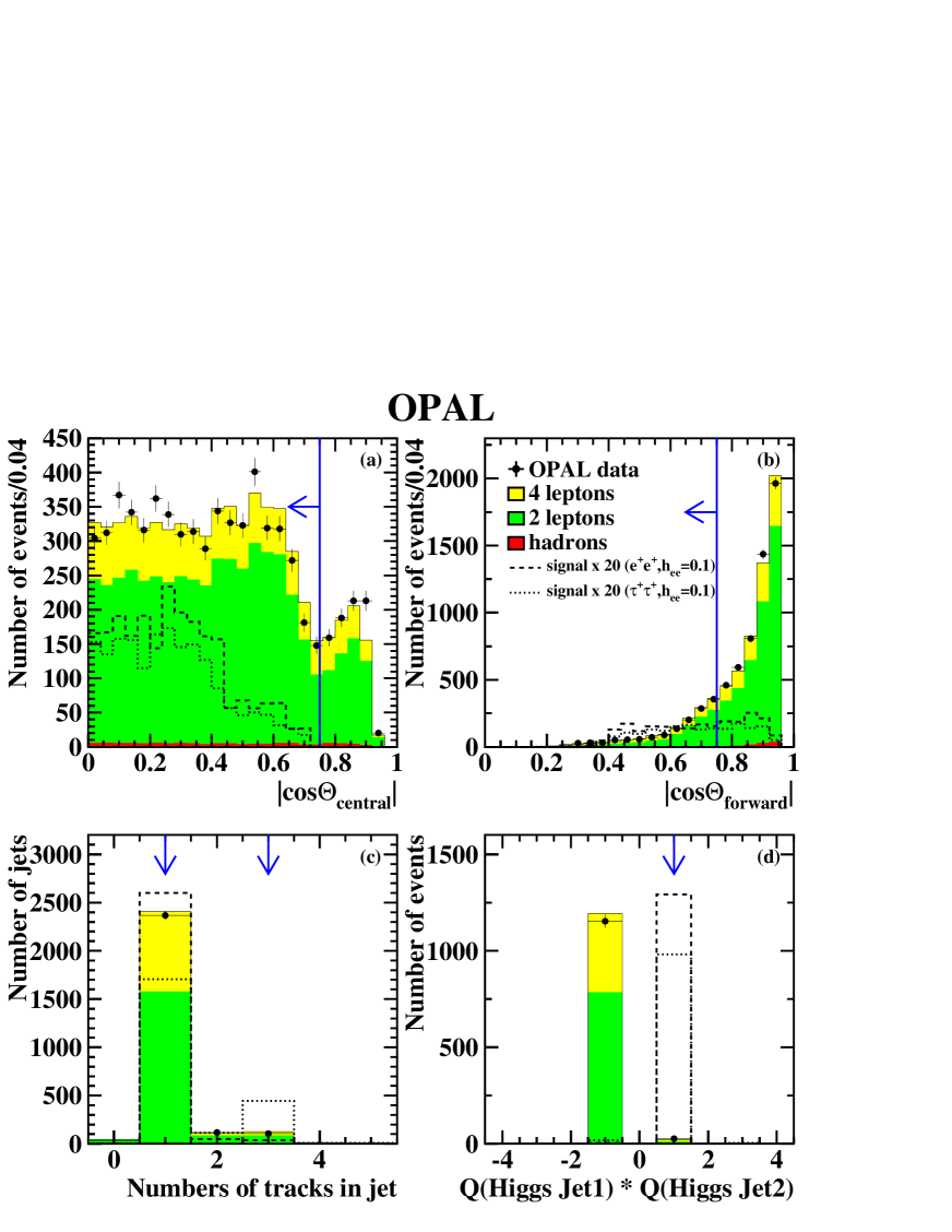
Figure 3: Examples of some of the quantities used in the two-lepton analysis selection shown immediately before the corresponding cut is applied (see Section 3.2). The absolute values of the cosines of the polar angle of the more central and the more forward Higgs boson candidate jets are shown in (a) and (b), the number of charged tracks in each of the two ${\rm H}^{\pm\pm}$ candidate jets in (c), and the product of the reconstructed charges of the two ${\rm H}^{\pm\pm}$ candidate jets in (d). The points with error bars indicate the OPAL data and the shaded regions indicate the background expectation. Note that “hadrons” includes both ${\rm q\bar{q}}(\gamma)$ and hadronic events from all 4-fermion processes. Two example signal expectations for a 130 GeV doubly-charged Higgs boson are also shown normalised to a cross-section corresponding to ${\rm h_{ee}}=0.1$ scaled by a factor 20, assuming either a 100% ${\rm H}^{\pm\pm}\rightarrow\rm ee$ branching ratio (dashed line) or a 100% ${\rm H}^{\pm\pm}\rightarrow\tau\tau$ branching ratio (dotted line). The cut requirements are indicated by the arrows.

• The polar angle of each jet must satisfy $|\cos\theta|<0.75$. The ${\rm H}^{\pm\pm}$ candidate jet polar angles are plotted in Figures 3(a) and (b) after cuts (2.1)–(2.4).

• Each jet associated to the ${\rm H}^{\pm\pm}$ must have either one or three charged tracks. The number of charged tracks is plotted in Figure 3(c) after cuts (2.1)–(2.5).

• Defining the sum of the track charges within each jet as the “jet charge”, the product of the charges of the two jets must be equal to $+1$. This value is plotted in Figure 3(d) after cuts (2.1)–(2.6).

The requirements for the three-lepton analysis are:

• The preselection is identical to that in cut (2.1) except that exactly three reconstructed jets are required. The two jets which have the highest reconstructed mass, as described in cut (3.3), have to satisfy $|\cos\theta|<$ 0.95 and must not be precisely back-to-back (within 5^∘). There is no $|\cos\theta|$ requirement for the third jet. Finally, the sum of the energies of the three jets reconstructed in the event must be greater than 20% of $\sqrt{s}$.

• Ordering the measured jet energies by their magnitude ($E_{\rm jet1}>E_{\rm jet2}>E_{\rm jet3}$), the following requirements are made:

  • $E_{\rm jet1}>0.1\sqrt{s}$;

  • $E_{\rm jet2}>0.05\sqrt{s}$;

  • $E_{\rm jet3}>0.025\sqrt{s}$ or it must contain at least one good charged track;

  • $E_{\rm jet1}<0.995E_{\rm beam}$;

  • $E_{\rm jet1}+E_{\rm jet2}+E_{\rm jet3}<0.95\sqrt{s}$.

• The jet energies are determined assuming that the measured jet direction is the same as the initial lepton direction for each of the reconstructed jets and that the missing electron or positron is recoiling along the beam axis. Using energy and momentum conservation to give four constraint equations, the four jet energies can be inferred (the lepton masses are neglected). Using this improved determination of the jet energies, the invariant masses are calculated for the three possible di-jet systems that can be constructed from the observed jets, and the two jets having the largest di-jet mass are considered as the ${\rm H}^{\pm\pm}$ candidate jets with a “reconstructed Higgs boson mass” $M_{\rm rec}$. The loss due to this assumption is negligible for ${\rm H}^{\pm\pm}$ masses above 110 GeV, and is taken into account in the signal efficiency calculation. Since this search concentrates on the region above the mass limit from pair creation, it is further required that $M_{\rm rec}$ satisfy $M_{\rm rec}>$ 80 GeV. Typical mass resolutions are about 1 GeV for ee and $\mu\mu$ modes, and about 4 GeV for $\tau\tau$ decays. Note that in the latter case, no mass reconstruction from the jet energies would have been possible without this procedure, due to the undetected neutrinos.

• Bhabha scattering is rejected by requiring that the acollinearity angle between the two ${\rm H}^{\pm\pm}$ candidate jets satisfies $\phi_{\rm acol}>15^{\circ}$.

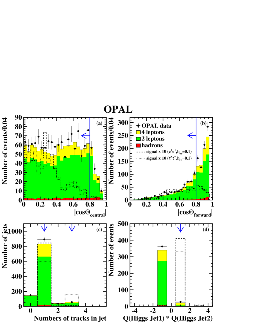
Figure 4: Examples of some of the quantities used in the three-lepton analysis selection shown immediately before the corresponding cut is applied (see Section 3.2). The absolute values of the cosines of the polar angle of the more central and the more forward Higgs boson candidate jets are shown in (a) and (b), the number of charged tracks in each of the two ${\rm H}^{\pm\pm}$ candidate jets in (c), and the product of the reconstructed charges of the two ${\rm H}^{\pm\pm}$ candidate jets in (d). The points with error bars indicate the OPAL data and the shaded regions indicate the background expectation. Note that “hadrons” includes both ${\rm q\bar{q}}(\gamma)$ and hadronic events from all 4-fermion processes. Two example signal expectations for a 130 GeV doubly-charged Higgs boson are also shown normalised to a cross-section corresponding to ${\rm h_{ee}}=0.1$ scaled by a factor 10, assuming either a 100% ${\rm H}^{\pm\pm}\rightarrow\rm ee$ branching ratio (dashed line) or a 100% ${\rm H}^{\pm\pm}\rightarrow\tau\tau$ branching ratio (dotted line). The cut requirements are indicated by the arrows.

• The polar angle of each jet associated to the ${\rm H}^{\pm\pm}$ must satisfy $|\cos\theta|<0.80$. The ${\rm H}^{\pm\pm}$ candidate jet polar angles are plotted in Figures 4(a) and (b) after cuts (3.1)–(3.4).

• Each jet associated to the ${\rm H}^{\pm\pm}$ must have either one or three charged tracks. The number of charged tracks is plotted in Figure 4(c) after cuts (3.1)–(3.5).

• Defining the sum of the track charges within each jet as the “jet charge”, the product of the charges of the two jets associated with the ${\rm H}^{\pm\pm}$ must be equal to $+1$. This value is plotted in Figure 4(d) after cuts (3.1)–(3.6).

The results are summarised in Table 2. The numbers of observed and expected events agree well after each cut in both analyses.

Two-lepton analysis
Cut	Data	Total	$\ell^{+}\ell^{-}$	4-$\ell$	‘$\gamma\gamma$’	${\rm q\bar{q}}$	‘$\gamma\gamma$’	Efficiency [%]
		Bkg.			$\rm ee\ell\ell$		$\rm eeqq$
								ee	$\mu\mu$	$\tau\tau$
(2.1)	19612	17659.3	13776.9	1249.6	2249.7	173.3	209.9	45.7	45.9	41.5
(2.2)	15168	14731.3	11381.3	1118.7	1971.5	158.1	101.8	44.3	39.1	36.4
(2.3)	13455	13002.6	10855.6	988.1	1026.5	120.8	11.6	44.3	39.0	35.0
(2.4)	6681	6685.9	5025.5	774.0	777.5	100.1	8.7	41.0	36.3	32.6
(2.5)	1318	1353.4	890.6	325.9	124.3	12.5	0.1	23.8	24.3	20.3
(2.6)	1181	1216.2	792.6	299.5	121.4	2.7	0.0	23.0	23.9	17.9
(2.7)	27	22.1	10.4	2.7	8.5	0.5	0.0	22.9	23.8	17.5
		$\pm$1.7	$\pm$1.3	$\pm$0.2	$\pm$1.1	$\pm$0.1	$\pm$0.0	$\pm$1.9	$\pm$2.0	$\pm$2.0
								(64.6)	(67.3)	(49.1)

Three-lepton analysis
Cut	Data	Total	$\ell^{+}\ell^{-}$	4-$\ell$	‘$\gamma\gamma$’	${\rm q\bar{q}}$	‘$\gamma\gamma$’	Efficiency [%]
		Bkg.			$\rm ee\ell\ell$		$\rm eeqq$
								ee	$\mu\mu$	$\tau\tau$
(3.1)	40948	40899.7	7422.7	467.9	27011.1	260.1	5738.0	34.1	36.2	33.3
(3.2)	3203	2816.0	1685.9	153.3	778.9	63.1	134.8	22.7	24.0	21.1
(3.3)	2031	1912.0	1557.9	100.5	199.4	44.4	9.8	22.7	24.0	20.0
(3.4)	1359	1247.1	939.8	83.2	182.2	32.5	9.3	21.8	23.4	19.5
(3.5)	572	538.3	427.4	41.4	55.5	13.3	0.7	15.5	17.8	14.1
(3.6)	390	361.8	273.4	29.9	52.5	5.8	0.2	14.7	17.3	12.6
(3.7)	28	22.3	4.4	4.0	13.3	0.5	0.1	14.6	17.2	11.9
		$\pm$1.6	$\pm$0.7	$\pm$0.3	$\pm$1.4	$\pm$0.1	$\pm$0.0	$\pm$2.0	$\pm$2.0	$\pm$2.1
								(41.0)	(48.8)	(33.4)

Sum
$\sum$	55	44.4	14.8	6.8	21.8	1.0	0.1	37.5	41.0	29.3
		$\pm$2.0	$\pm$1.3	$\pm$0.3	$\pm$1.5	$\pm$0.1	$\pm$0.0	$\pm$2.8	$\pm$2.8	$\pm$2.9
								(105.6)	(116.1)	(82.5)

Table 2: The number of remaining events in the data after each cut, and the number expected from Standard Model background sources. Also shown are the efficiencies of expected signal events for a 130 GeV doubly-charged Higgs boson assuming ee, $\mu\mu$ or $\tau\tau$ decays. The number of expected signal events for ${\rm h_{ee}}=0.1$ is shown in brackets assuming 100% branching ratio for the given decay mode. The errors due to Monte Carlo statistics are also listed for events surviving the full analysis.

3.3 Systematic Uncertainties

The largest background in the selection is from processes with four charged leptons in the final state, particularly from multi-peripheral “two-photon” processes. Of concern is the fact that, in our standard Monte Carlo background samples available at all centre-of-mass energies, the multi-peripheral diagrams are treated with specialised event generators which neglect interference with non-multi-peripheral diagrams. Special samples of the full set of ${\rm e^{+}e^{-}}\rightarrow{\rm e^{+}e^{-}}\ell^{+}\ell^{-}$ diagrams, including interference, were prepared using grc4f2.2[14] at $\sqrt{s}=206$ GeV to study this effect. The background using the full set of ${\rm e^{+}e^{-}}\ell^{+}\ell^{-}$ diagrams including interference is in both analyses about $25$% lower than our standard set of Monte Carlo generators. While grc4f2.2 includes interference effects, it has other differences with respect to our standard background simulations and cannot be used as the primary sample. We therefore simply assign a 25% systematic uncertainty on the ${\rm e^{+}e^{-}}\ell^{+}\ell^{-}$ background according to this cross-check. Monte Carlo modelling of the variables used in the selection cuts can also induce systematic effects. The possible level of mismodelling is assessed by comparing data and background Monte Carlo for each variable after the preselection (cut (2.1) and (3.1), respectively) where the contribution from a signal would be negligible. Differences between the data and background Monte Carlo simulation are used to define a possible shift in each variable, and then the systematic uncertainties are evaluated by varying the cuts by these shifts. Both the final expected background and signal efficiencies are re-calculated with these shifted cuts, and the full differences from the nominal values are assigned as systematic uncertainties.

The uncertainty of charge identification, used in cuts (2.7/3.7) in Section 3.2 to reject a significant fraction of the background, is estimated from a clean sample of Bhabha events selected by changing the cuts as follows. The cuts (2.2)c and (3.2)d are not applied. Cuts (2.2)d and (3.2)e are changed from $E_{\rm jet1}+E_{\rm jet2}(+E_{\rm jet3})<0.95\sqrt{s}$ to $E_{\rm jet1}+E_{\rm jet2}(+E_{\rm jet3})>0.95\sqrt{s}$. This sample consists mainly of Bhabha events and has no overlap with the search sample. The fraction of like-sign electron pairs is 2.0% in data and 1.7% in Monte Carlo. The systematic uncertainties on the background and signal efficiencies are evaluated by randomly changing the sign of the charge for 0.15% of the tracks, in order to increase the fraction of fake like-sign events by 0.3%, the observed difference between data and Monte Carlo in Bhabha sample. The full differences between the new background and efficiencies and the nominal ones are taken as systematic uncertainties.

The systematic uncertainties are summarised in Table 3. Additional systematic uncertainties, such as on the integrated luminosity, are negligible.

		2-lepton analysis:		3-lepton analysis:
Quantity	Variation	$\Delta$ Bkg	$\Delta$ Sig	$\Delta$ Bkg	$\Delta$ Sig
		(%)	(%)	(%)	(%)
Jet $\cos{\theta}$	$\pm 0.5^{\circ}$	8	1	7	1
Jet Energy	$\pm$1%	1	1	2	1
$\phi_{\rm acol}$	$\pm 0.5^{\circ}$	2	1	1	1
Charge Misidentification	0.15%	14	1	4	1
Background Modelling	(see text)	25	–	25	–
Monte Carlo Statistics	–	8	10	7	14
Quadratic Sum		31	10	27	14

Table 3: Systematic uncertainties on signal and background.

3.4 Direct Search Results

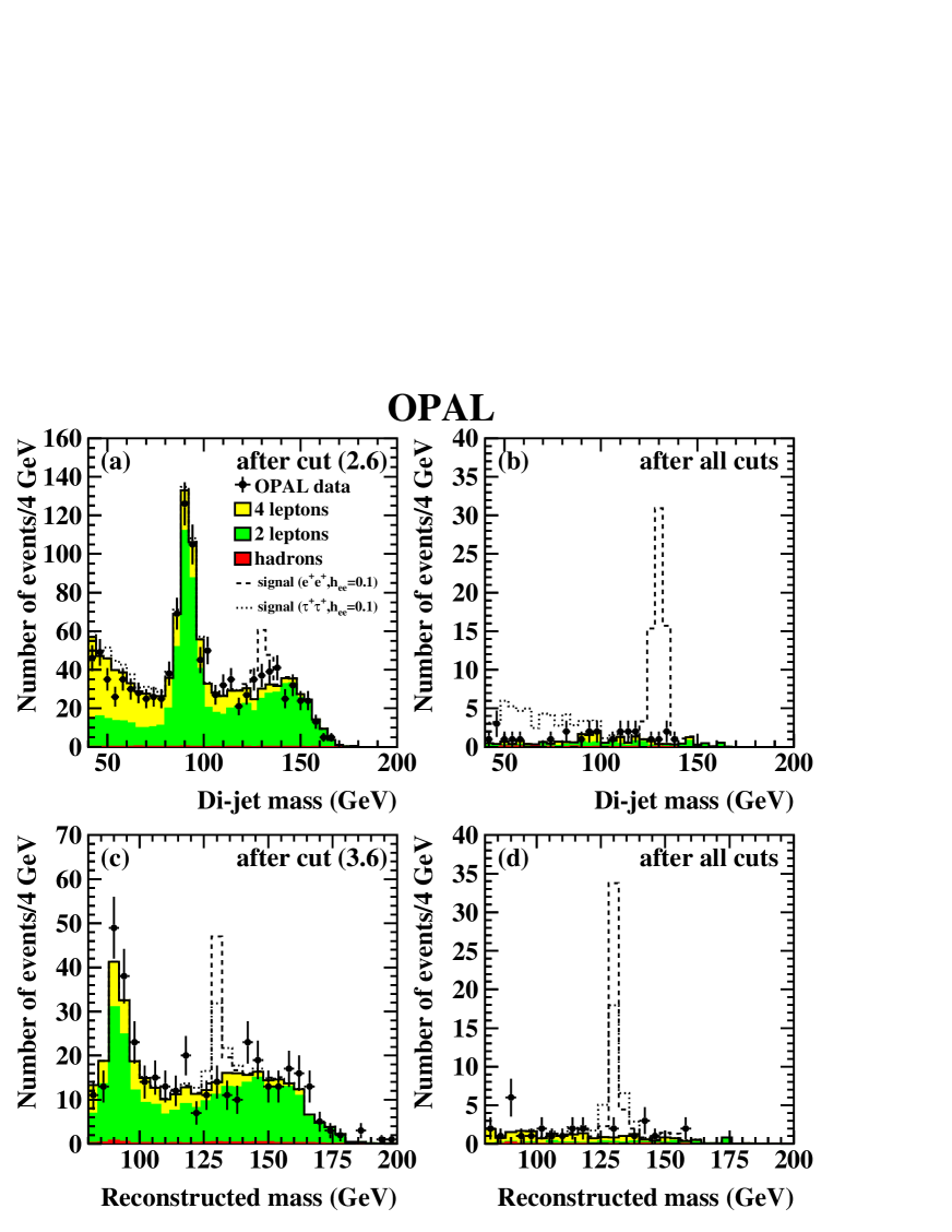
Figure 5: The reconstructed ${\rm H}^{\pm\pm}$ candidate mass distributions. The invariant di-jet mass is shown for the 2-lepton analysis both before and after the like-signed jet requirement (cut (2.7)) in (a) and (b), respectively. For the 3-lepton analysis, the reconstructed ${\rm H}^{\pm\pm}$ mass using the jet angles as discussed in the text, is shown before and after cut (3.7) in (c) and (d), respectively. The points with error bars indicate the OPAL data and the shaded regions indicate the background expectation. Note that “hadrons” includes both ${\rm q\bar{q}}(\gamma)$ and hadronic events from all 4-fermion processes. Two example signal expectations for a 130 GeV doubly-charged Higgs boson are also shown normalised to a cross-section corresponding to ${\rm h_{ee}}=0.1$, assuming either a 100% ${\rm H}^{\pm\pm}\rightarrow\rm ee$ branching ratio (dashed line) or a 100% ${\rm H}^{\pm\pm}\rightarrow\tau\tau$ branching ratio (dotted line). Note that due to the undetected neutrinos from the tau-lepton decay there is no peak in the ${\rm H}^{\pm\pm}\rightarrow\tau\tau$ signal sample of the 2-lepton analysis ((a) and (b)).

In the two-lepton analysis the invariant mass of the two jets is calculated using the measured jet energies and directions, because it is not possible to use the “angle-based” kinematic reconstruction described in section 3.2 for the three-lepton analysis. The mass distribution is shown in Figure 5 for events passing all cuts except the like-signed charge requirement (a), and also with all cuts applied (b). No excess of events which could imply the presence of a signal is observed in the data.

In the three-lepton analysis we calculate the ${\rm H}^{\pm\pm}$ candidate reconstructed masses, $M_{\rm rec}$,shown in Figure 5, using the “angle-based” kinematic reconstruction described in item (3.3) in Section 3.2. The mass distributions are shown both for events passing all cuts except the like-signed charge requirement (c), and also with all cuts applied (d). Additionally, as a cross-check to ensure that no di-jet mass peak present after the event reconstruction is reduced by the angle-based method, the largest di-jet mass calculated from only the track and cluster information (Section 3.2) was examined. No excess of events which could imply the presence of a signal is observed in the data.

Limits are set on the ${\rm H}^{\pm\pm}$ Yukawa coupling ${\rm h_{ee}}$, assuming that the sum of the branching fractions of the ${\rm H}^{\pm\pm}$ to all lepton flavour combinations is 100%. The efficiency for an arbitrary Higgs boson mass is determined by linear interpolation between the simulated signal Monte Carlo samples. The number of observed events, together with the number of expected signal and background events from both the two-lepton and three-lepton analyses are combined using the likelihood ratio method described in [28], which incorporates the systematic uncertainties into the limits using a numerical convolution technique. For the purpose of extracting the limits, a $\pm 10$ GeV “sliding mass window” around the hypothetical Higgs boson mass is used. Events within this window are counted in data and Monte Carlo simulation. The hypothetical Higgs boson mass is varied in 1 GeV steps. The width of the mass window is chosen such that it contains most of the expected signal events. A small efficiency correction, typically around 5% for ee and $\mu\mu$ and 10% for $\tau\tau$, due to this window is applied. In the two-lepton analysis for any channel containing $\tau$ leptons no mass window cut is applied, because in this channel it is not possible to reconstruct the correct mass of the doubly-charged Higgs boson due to the undetected neutrinos.

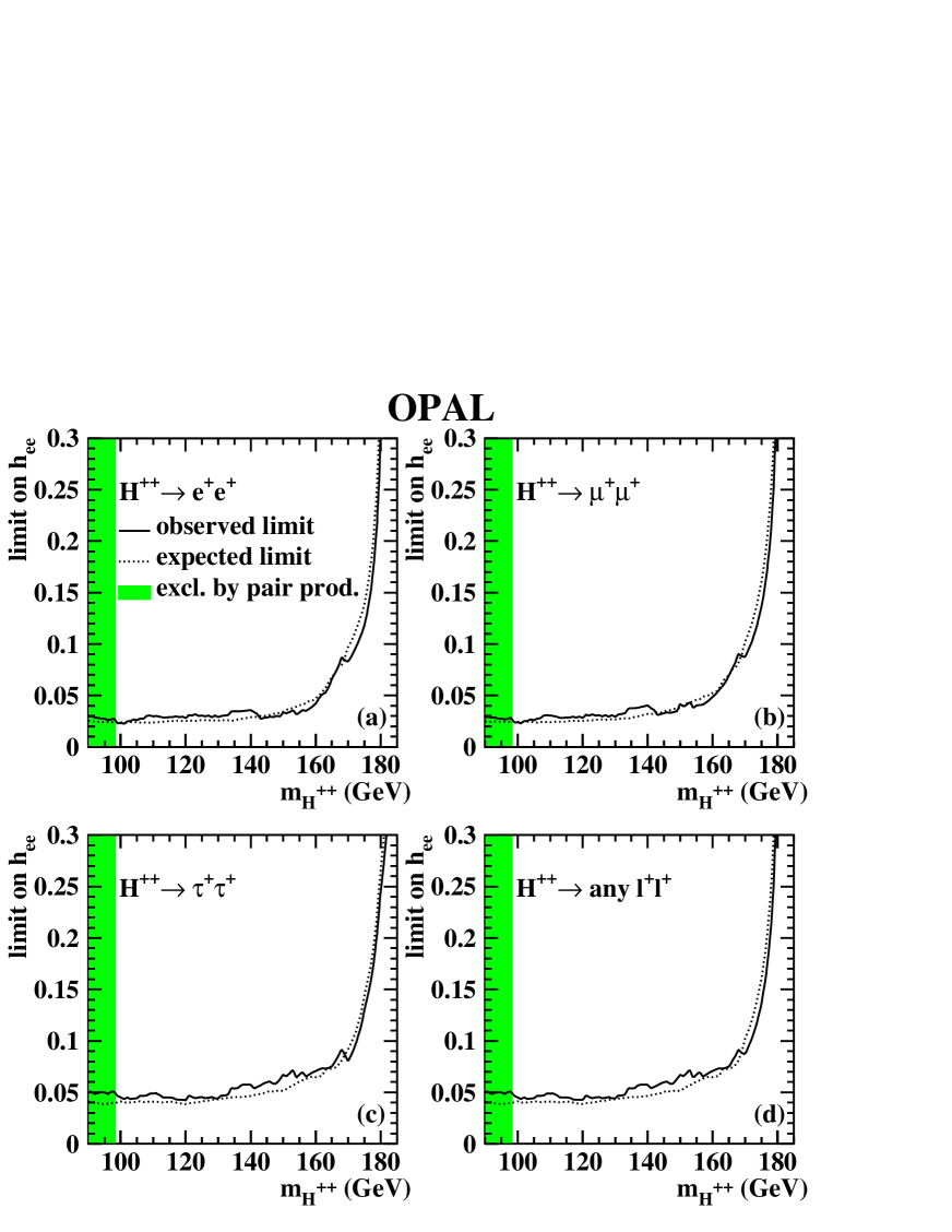
Figure 6: Limits at the 95% confidence level on the Yukawa coupling ${\rm h_{ee}}$ assuming a 100% branching fraction of the ${\rm H}^{\pm\pm}$ to (a) ee, (b) $\mu\mu$ and (c) $\tau\tau$. The limits are calculated with the combined results of the two-lepton and three-lepton analysis. In (b) and (c), the limits should be regarded as valid in the large branching fraction limit, since non-zero ${\rm h_{ee}}$ implies a non-zero electron branching fraction (see text). Since the ee and $\mu\mu$ efficiencies and mass resolutions are very similar, figures (a) and (b) are almost identical. The median expected limits assuming only Standard Model processes are shown by the dotted lines, while the actual limits inferred from the data are shown by the solid lines. In figure (d) the limit for arbitrary lepton flavour combinations (ee, e$\mu$, e$\tau$, $\mu\mu$, $\mu\tau$ and $\tau\tau$) is shown. It is determined by the pure $\tau\tau$ case except for masses in excess of 170 GeV. The shaded regions for masses below 98.5 GeV are excluded in Left-Right symmetric models by the OPAL pair production search [6].

The limits on ${\rm h_{ee}}$ are calculated using the efficiencies determined from the PYTHIA Monte Carlo samples and the production cross-sections are determined in a consistent manner using PYTHIA (see discussion in Section 3.1). No systematic uncertainty is assigned for theoretical uncertainties. The 95% confidence level limits on ${\rm h_{ee}}$ from combining both analyses are shown in Figure 6(a)–(c) assuming a branching fraction of the doubly-charged Higgs boson into ee, $\mu\mu$, $\tau\tau$ of 100%, respectively. Strictly, due to the production mechanism involving non-zero ${\rm h_{ee}}$, exactly 100% $\mu\mu$ or $\tau\tau$ decays are not possible, therefore the latter limits should be considered for the case $\mathrm{h}_{\mu\mu,\tau\tau}\gg{\rm h_{ee}}$. In Figure 6(d), for each mass the highest limit from all possible lepton flavour combinations is shown. An upper limit on ${\rm h_{ee}}<$ 0.071 is inferred for $M({\rm H}^{\pm\pm})<$ 160 GeV at the 95% confidence level, which is valid for all possible lepton flavour combinations in the decays. The limit is determined by the pure $\tau\tau$ case except for masses in excess of 170 GeV. For the case of pure ee decays the limit is ${\rm h_{ee}}<$ 0.042, and for $\mu\mu$ decays ${\rm h_{ee}}<$ 0.049, both for $M({\rm H}^{\pm\pm})<$ 160 GeV. For the mixed flavour decay modes e$\mu$, e$\tau$, and $\mu\tau$ the limit is between those for pure decays of the two involved flavours.

4 Indirect Search

Doubly-charged Higgs bosons would contribute to Bhabha scattering via $t$-channel exchange as shown in Figure 2. The Born level differential cross-section for Bhabha scattering including the exchange of a doubly-charged Higgs boson with right-handed couplings has been calculated in [5]. At high masses, $M({\rm H}^{\pm\pm})\gg\sqrt{s}$, the cross-section is identical to that derived for four-fermion contact interactions with right-handed currents [29] ($\eta_{\rm RR}=1$, $\eta_{\rm LL}=\eta_{\rm LR}=0$), with the replacement of $g/\Lambda$ by ${\rm h_{ee}}/M({\rm H}^{\pm\pm})$ where ${\rm h_{ee}}$ is the Higgs coupling to electrons. At values of $M({\rm H}^{\pm\pm})$ comparable to the centre-of-mass energy, this correspondence is modified by the inclusion of a propagator term. For comparison with the experimental data, QED radiative corrections are applied to the Born level terms for doubly-charged Higgs boson exchange and interference with Standard Model processes given in [5] using the program MIBA [30]. Initial state radiation is calculated up to ${\cal O}(\alpha^{2})$ in the leading log approximation with soft photon exponentiation, and the ${\cal O}(\alpha)$ leading log final state QED correction is applied. The BHWIDE [21] program is used to calculate the Standard Model contribution to the differential cross-section. The theoretical predictions are calculated using the same acceptance cuts as are applied to the data.

This analysis uses OPAL measurements of the differential cross-section for ${\rm e^{+}e^{-}}\rightarrow{\rm e^{+}e^{-}}$ at centre-of-mass energies of 183–209 GeV[31, 32]. The data between 203 GeV and 209 GeV are grouped into two sets with mean energies of approximately 205 GeV and 207 GeV. The total integrated luminosity of the data amounts to 688.4 pb^-1. These measurements cover the range $|\cos\theta|<0.9$, in 15 bins of $\cos\theta$ (as defined in [32]), and correspond to $\theta_{\mathrm{acol}}<10^{\circ}$ where $\theta_{\mathrm{acol}}$ is the acollinearity angle between electron and positron. It is verified that the effect of doubly-charged Higgs boson exchange on the low-angle Bhabha scattering cross-section has a negligible effect on the luminosity determination even for values of ${\rm h_{ee}}$ a few times larger than excluded by this measurement.

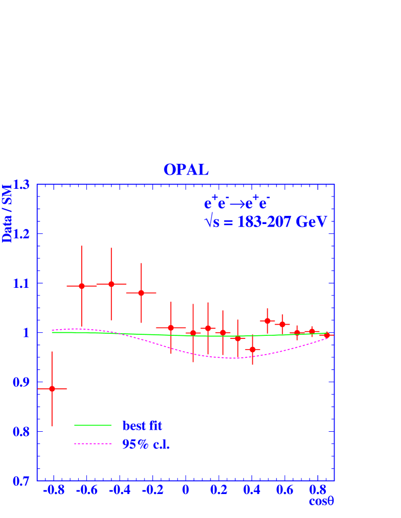
Figure 7: Ratio of the measured luminosity-weighted average differential cross-section for ${\rm e^{+}e^{-}}\rightarrow{\rm e^{+}e^{-}}$ at 183–207 GeV to the Standard Model prediction. The points with error bars show the OPAL data, while the curves show theoretical predictions for a doubly-charged Higgs boson mass of 130 GeV. The solid curve corresponds to the best fit to all data, the dashed curve corresponds to a coupling equal to the 95% confidence level limit.

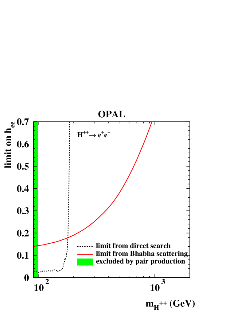
Figure 9: Limits at the 95% confidence level on the Yukawa coupling ${\rm h_{ee}}$ assuming a 100% branching fraction of the ${\rm H}^{\pm\pm}\rightarrow ee$. The direct limit is calculated with the combined results of the two-lepton and three-lepton analyses. The indirect limit on ${\rm h_{ee}}$ obtained from Bhabha scattering described in Section 4 is also shown. The shaded regions for masses below 98.5 GeV are excluded in Left-Right Symmetric models by the OPAL pair production search [6].

The measured differential cross-sections are fitted with the theoretical prediction using a $\chi^{2}$ fit. The fit is performed for fixed values of the doubly-charged Higgs boson mass between 80 GeV and 2000 GeV, allowing the square of the coupling, ${\rm h_{ee}^{2}}$, to vary. Although only ${\rm h_{ee}^{2}}>0$ is physically meaningful, in order to allow for the case where the data fluctuate in the opposite direction to that expected for doubly-charged Higgs boson exchange, both positive and negative values of ${\rm h_{ee}^{2}}$ are allowed in the fit. Experimental and theoretical systematic uncertainties and their correlations are treated as discussed in [32]. The fitted values of ${\rm h_{ee}^{2}}$ are consistent with zero for all masses, indicating that the data are consistent with the Standard Model prediction. For example, for a mass of 130 GeV the fitted value of ${\rm h_{ee}^{2}}$ is 0.003$\pm$0.011, and the fit has a $\chi^{2}$ of 97.0 for 119 degrees of freedom. Figure 7 shows the ratio of the measured luminosity-weighted average differential cross-section at 183–207 GeV to the Standard Model prediction, together with the results of the fit. 95% confidence level limits on the coupling as a function of mass were derived by integrating the likelihood function obtained from $\chi^{2}$ over the region ${\rm h_{ee}^{2}}>0$, and are shown in Figure 8. The limits are considerably more stringent than those derived from PEP and PETRA data [5]. Figure 9 shows the limits from the indirect search together with those from the direct search. The indirect limits are less restrictive than those from the direct search at low masses, but extend to much higher masses.

5 Conclusion

A direct search for the single production of doubly-charged Higgs bosons has been performed. No evidence for the existence of ${\rm H}^{\pm\pm}$ is observed. Upper limits are determined on the Higgs Yukawa coupling to like-signed electron pairs, ${\rm h_{ee}}$. A 95% confidence level upper limit of ${\rm h_{ee}}<$ 0.071 is inferred for $M({\rm H}^{\pm\pm})<$ 160 GeV assuming that the sum of the branching fractions of the ${\rm H}^{\pm\pm}$ to all lepton flavour combinations is 100%. Additionally, indirect constraints on ${\rm h_{ee}}$ for $M({\rm H}^{\pm\pm})<$ 2 TeV are derived from Bhabha scattering where the ${\rm H}^{\pm\pm}$ would contribute via $t$-channel exchange for $M({\rm H}^{\pm\pm})<$ 2 TeV. These are the first results on both the single production search and constraints from Bhabha scattering reported from LEP.

Acknowledgements

The authors would like to thank André Schöning for suggesting that we perform this search, Steve Godfrey and Pat Kalyniak for valuable discussions and assistance during the preparation of this paper, and also Emmanuelle Perez for a helpful hint about the PYTHIA code.

We particularly wish to thank the SL Division for the efficient operation of the LEP accelerator at all energies and for their close cooperation with our experimental group. In addition to the support staff at our own institutions we are pleased to acknowledge the
Department of Energy, USA,
National Science Foundation, USA,
Particle Physics and Astronomy Research Council, UK,
Natural Sciences and Engineering Research Council, Canada,
Israel Science Foundation, administered by the Israel Academy of Science and Humanities,
Benoziyo Center for High Energy Physics,
Japanese Ministry of Education, Culture, Sports, Science and Technology (MEXT) and a grant under the MEXT International Science Research Program,
Japanese Society for the Promotion of Science (JSPS),
German Israeli Bi-national Science Foundation (GIF),
Bundesministerium für Bildung und Forschung, Germany,
National Research Council of Canada,
Hungarian Foundation for Scientific Research, OTKA T-038240, and T-042864,
The NWO/NATO Fund for Scientific Research, the Netherlands.

Figure 8: Limits at the 95% confidence level on the Yukawa coupling ${\rm h_{ee}}$ as a function of $M({\rm H}^{\pm\pm})$ derived from Bhabha scattering data (solid line) for an ${\rm H}^{\pm\pm}$ coupling to right-handed particles. Limits at 90% confidence level derived from PEP and PETRA data [5] are shown, as a dashed line, for comparison.

References

-
[1]
J.C. Pati and A. Salam, Phys. Rev. D10 (1974) 275;
R.N. Mohapatra and J.C. Pati, Phys. Rev. D11 (1975) 566, 2558;
G. Senjanovic and R.N. Mohapatra, Phys. Rev. D12 (1975) 1502;
R.N. Mohapatra and R.E. Marshak, Phys. Lett. B91 (1980) 222;
R.N. Mohapatra and D. Sidhu, Phys. Rev. Lett. 38 (1977) 667. - [2] G.B. Gelmini and M. Roncadelli, Phys. Lett. B99 (1981) 411.
-
[3]
N. Arkani-Hamed, A. G. Cohen and H. Georgi,
Phys. Lett. B 513 (2001) 232;
N. Arkani-Hamed, A. G. Cohen, T. Gregoire and J. G. Wacker, JHEP 0208 (2002) 020;
N. Arkani-Hamed et al. , JHEP 0208 (2002) 021;
T. Han, H. E. Logan, B. McElrath and L. T. Wang, Phys. Rev. D 67 (2003) 095004. -
[4]
C. S. Aulakh, A. Melfo and G. Senjanovic, Phys. Rev. D57 (1998) 4174;
Z. Chacko and R. N. Mohapatra, Phys. Rev. D58 (1998) 15003;
B. Dutta and R. N. Mohapatra, Phys. Rev. D59 (1999) 15018. - [5] M.L. Swartz, Phys. Rev. D40 (1989) 1521.
- [6] OPAL Collab., G. Abbiendi et al., Phys. Lett. B526 (2002) 221.
- [7] DELPHI Collab., J. Abdallah et al., Phys. Lett. B 552 (2003) 127.
- [8] G. Barenboim, K. Huitu, J. Maalampi and M. Raidal, Phys. Lett. B394 (1997) 132.
- [9] S. Godfrey, P. Kalyniak and N. Romanenko, Phys. Lett. B545 (2002) 361.
-
[10]
OPAL Collab., K. Ahmet et al., Nucl. Instr. Meth. A305 (1991) 275;
S. Anderson et al., Nucl. Instr. Meth. A403 (1998) 326;
B.E. Anderson et al., IEEE Trans. on Nucl. Science 41 (1994) 845;
G. Aguillion et al., Nucl. Instr. Meth. A417 (1998) 266. -
[11]
T. Sjöstrand, Comp. Phys. Comm. 39 (1986) 347;
T. Sjöstrand, PYTHIA 5.7 and JETSET 7.4 Manual, CERN-TH 7112/93;
T. Sjöstrand et al., Computer Phys. Commun. 135 (2001) 238. - [12] A. Pukhov et al., ‘CompHEP: A package for evaluation of Feynman diagrams and integration over multi-particle phase space. User’s manual for version 33’, arXiv:hep-ph/9908288.
-
[13]
M. Skrzypek et al., Comp. Phys. Comm. 94 (1996) 216;
M. Skrzypek et al., Phys. Lett. B372 (1996) 286. - [14] J. Fujimoto et al., Comp. Phys. Comm. 100 (1997) 128.
- [15] J.A.M. Vermaseren, Nucl. Phys. B229 (1983) 347.
- [16] F.A. Berends, P.H. Daverveldt and R. Kleiss, Nucl. Phys. B253 (1985) 421; Comp. Phys. Comm. 40 (1986) 271, 285, 309.
- [17] R. Engel and J. Ranft, Phys. Rev. D 54 (1996) 4244.
- [18] G. Marchesini et al., Comp. Phys. Comm. 67 (1992) 465.
- [19] S. Jadach, B.F.L. Ward and Z. Wa̧s, Phys. Lett. B449 (1999) 97.
- [20] G. Montagna, M. Moretti, O. Nicrosini and F. Piccinini, Nucl. Phys. B541 (1999) 31.
- [21] S. Jadach, W. Płaczek and B.F.L. Ward, Phys. Lett. B390 (1997) 298.
- [22] D. Karlen, Nucl. Phys. B289 (1987) 23.
- [23] F.A. Berends and R. Kleiss, Nucl.Phys. B186 (1981) 22.
- [24] J. Allison et al., Nucl. Instr. Meth. A317 (1992) 47.
- [25] OPAL Collab., K. Ackerstaff et al., Eur. Phys. J. C2 (1998) 213.
- [26] OPAL Collab., G. Alexander et al., Z.Phys. C52 (1991) 175.
- [27] OPAL Collab., R. Akers et al., Z.Phys.C63 (1994) 197.
- [28] T. Junk, Nucl.Instrum.Meth. A434 (1999) 435.
- [29] E. Eichten, K. Lane and M. Peskin, Phys. Rev. Lett. 50 (1983) 811.
- [30] M. Martinez and R. Miquel, Z.Phys. C53 (1992) 115.
- [31] OPAL Collab., G. Abbiendi et al., Eur. Phys. J. C6 (1999) 1.
- [32] OPAL Collab., G. Abbiendi et al., ‘Tests of the Standard Model and Constraints on New Physics from Measurements of Fermion-pair Production at 189-209 GeV at LEP’, paper in preparation.