The BABAR Collaboration

A preliminary measurement of $|V_{cb}|$ and the branching fraction ${\cal B}(\bar{B^{0}}\rightarrow D^{*+}\ell^{-}\bar{\nu_{\ell}}$) has been performed based on a sample of about 55,700 $\bar{B^{0}}\rightarrow D^{*+}\ell^{-}\bar{\nu_{\ell}}$ decays recorded with the BABAR  detector. The decays are identified in the $D^{*+}\rightarrow D^{0}\pi^{+}$ final state, with the $D^{0}$ reconstructed in three different decay modes. The differential decay rate is measured as a function of the relativistic boost of the $D^{*+}$ in the ${\bar{B^{0}}}$ rest frame. The value of the differential decay rate at ‘zero recoil’, namely the point at which the $D^{*+}$ is at rest in the ${\bar{B^{0}}}$ frame, is predicted in Heavy Quark Effective Theory as a kinematic factor times ${\cal F}(1)|V_{cb}|$, where ${\cal F}$ is the unique form factor governing the decay. We extrapolate the measured differential decay rate to the zero recoil point and obtain ${\cal F}(1)|V_{cb}|=(34.03\pm 0.24\pm 1.31)\times 10^{-3}$. Using a theoretical calculation for ${\cal F}(1)$ we extract

$$|V_{cb}|=(37.27\pm 0.26\mathrm{(stat.)}\pm 1.43\mathrm{(syst.)}^{+1.5}_{-1.2}\mathrm{(theo.)})\times 10^{-3}.$$

From the integrated decay rate we obtain

$${\cal B}(\bar{B^{0}}\rightarrow D^{*+}\ell^{-}\bar{\nu_{\ell}})=(4.68\pm 0.03\pm 0.29)\%.$$

Contributed to the XXI^st International Symposium on Lepton and Photon Interactions at High Energies, 8/11 — 8/16/2003, Fermilab, Illinois USA

This work is dedicated to the memory of Paolo Poropat.

1 Introduction

In the framework of the Standard Model, the weak coupling between quarks of different flavors is described by the Cabibbo-Kobayashi-Maskawa (CKM) matrix. Its elements are not predicted by theory, but are constrained only to give a unitary matrix.

A precise measurement of $|V_{cb}|$, the element corresponding to the $b\rightarrow c$ transitions, is needed to determine whether the CKM matrix provides a quantitatively accurate description of the $C\!P$ violation observed in $B^{0}$ mesons. Progress in the phenomenological description of heavy flavor semileptonic decay allows the determination of $|V_{cb}|$ with small theoretical uncertainty, either from the inclusive process $b\rightarrow c\ell\bar{\nu}$, or from an analysis of the form factors in the decay $\bar{B^{0}}\rightarrow D^{*+}\ell^{-}\bar{\nu_{\ell}}$. The present measurement is based on the second approach [1].

The decay rate for the process is proportional to $|V_{cb}|^{2}$ and to the square of the hadronic matrix elements describing the transition from a $\kern 1.79993pt\overline{\kern-1.79993ptB}{}^{0}$ to a $D^{*+}$ meson. In the context of the Heavy Quark Effective Theory (HQET) [2], the matrix element is proportional to a single form factor ${\cal F}$($w$), where $w$ is the product of the $\kern 1.79993pt\overline{\kern-1.79993ptB}{}^{0}$ and $D^{*+}$ four-vector velocities. For ${w}=1$, the $D^{*+}$ is produced at rest in the $\kern 1.79993pt\overline{\kern-1.79993ptB}{}^{0}$ rest frame. Heavy-flavor symmetry predicts the normalization ${{\cal F}}(1)=1$ in the limit of an infinitely massive $b$-quark. Corrections to this prediction due to perturbative QCD have been computed up to second order in $\alpha_{\scriptscriptstyle S}$ [3] and the effect of finite $b$ and $c$ quark masses has been calculated in the framework of HQET, yielding ${{\cal F}}(1)=0.913^{+0.030}_{-0.035}$ [4].

A measurement of the differential decay rate near ${w}=1$ determines $|V_{cb}|$ with small theoretical uncertainty. The rate at ${w}=1$ is suppressed by phase space. Consequently, the differential rate d$\Gamma$/d$w$ is measured, where ${\cal F}$($w$) is parametrized using several different functional forms [5, 6] (see also discussion below), and is extrapolated to ${w}=1$. Results based on this approach have been reported by the ARGUS [7], Belle [8], and CLEO [9] collaborations operating at the $\mathchar 28935\relax$(4S) and by ALEPH [10, 11], DELPHI [12, 13] and OPAL [14] at LEP.

This paper presents preliminary results for the measurements of $|V_{cb}|$ and of the branching fraction ${\cal B}($$\bar{B^{0}}\rightarrow D^{*+}\ell^{-}\bar{\nu_{\ell}}$) performed on a sample of $\bar{B^{0}}\rightarrow D^{*+}\ell^{-}\bar{\nu_{\ell}}$ decays selected from events with a high momentum charged lepton $\ell^{-}$ and a ${D^{*+}}$ . The $D^{*+}$ is reconstructed from its decay to a charged pion and a $D^{0}$. This pion is produced with small momentum, and is commonly referred to as the slow pion ($\pi_{\rm slow}$).

This paper is organized as follows. The next section is dedicated to a brief description of the BABAR detector and of the data sets employed. Section 3 describes the event selection and the composition of the sample used for the measurement. The fit method and its results are described in Section 4; the evaluation of the systematic error is discussed in Section 4.4. Finally, Section  5 presents the conclusions and the comparison with other measurements of $|V_{cb}|$.

2 The BABAR Detector

The data were collected with the BABAR detector at the PEP-II asymmetric energy $e^{+}e^{-}$ storage ring [15]. The sample consists of 79.1 $\mbox{\,fb}^{-1}$ collected at a center-of-mass energy corresponding to the $\mathchar 28935\relax{(4S)}$ resonance (“on-resonance”), and 9.6 $\mbox{\,fb}^{-1}$ collected 40 $\mathrm{\,Me\kern-1.00006ptV}$ below the $\mathchar 28935\relax{(4S)}$ resonance (“off-resonance”) for continuum background studies. The on-resonance sample corresponds to $N_{\mathchar 28935\relax}=(85.9\pm 0.9)\times 10^{6}$ $\mathchar 28935\relax{(4S)}$ decays to $B\kern 1.79993pt\overline{\kern-1.79993ptB}{}$ mesons.

The BABAR detector is described in detail elsewhere [16]. The momenta of charged particles are measured using a combination of a five-layer silicon vertex tracker (SVT) and a 40-layer drift chamber (DCH) in a 1.5 T solenoidal magnetic field. A detector of internally-reflected Cherenkov radiation (DIRC) is used for charged-particle identification. Kaons are identified with a neural network based on the likelihood ratios calculated from d$E$/d$x$ measurements in the SVT and DCH, and from the information from the DIRC. A finely segmented CsI(Tl) electromagnetic calorimeter (EMC) is used to detect photons and neutral hadrons, and to identify electrons. Electron candidates are required to have a ratio of EMC energy to track momentum, EMC cluster shape, DCH d$E$/d$x$, and DIRC Cherenkov angle all consistent with the electron hypothesis. The instrumented flux return (IFR) contains resistive plate chambers for muon and long-lived neutral hadron identification. Muon candidates are required to have IFR hits located along the extrapolated DCH track, and energy deposition in the EMC and penetration length in the IFR consistent with a minimum ionizing particle.

3 Event Selection and Sample Composition

3.1 Event Selection

Events are selected that contain a fully-reconstructed $D^{*+}$ and an oppositely charged lepton. Those ${D^{*+}}\ell^{-}$ combinations not coming from the signal decay are suppressed by means of kinematic cuts.

A candidate lepton is searched for among all charged tracks with momentum greater than 1.2 GeV/$c$ in the $\mathchar 28935\relax{(4S)}$ rest frame. Electron candidates are selected with an efficiency of about 90% and a hadron misidentification probability of less than 0.2%. Muon candidates are selected with an efficiency of $\simeq 60$% and hadron misidentification probability is about 2%.

The $D^{*+}$ candidate is selected in the decay mode ${D^{*+}}\rightarrow D^{0}\pi^{+}$ and the $D^{0}$ meson is reconstructed in the three modes ${K^{-}\pi^{+}}$, ${K^{-}\pi^{+}\pi^{+}\pi^{-}}$, and ${K^{-}\pi^{+}\pi^{0}}$. The $\pi^{0}$ is reconstructed from two photons, each with energy larger than 30 $\mathrm{\,Me\kern-1.00006ptV}$, and must have a total energy larger than 200 $\mathrm{\,Me\kern-1.00006ptV}$ and an invariant mass between 119.2 and 150.0 ${\mathrm{\,Me\kern-1.00006ptV\!/}c^{2}}$. The invariant mass of the two photons is constrained to the $\pi^{0}$ mass and the pair is kept as a $\pi^{0}$ candidate if the $\chi^{2}$ probability of the fit exceeds 1%. Charged kaon candidates satisfy loose identification criteria for the ${K^{-}\pi^{+}}$ mode and tighter criteria for the ${K^{-}\pi^{+}\pi^{+}\pi^{-}}$ and ${K^{-}\pi^{+}\pi^{0}}$ modes. For the ${K^{-}\pi^{+}\pi^{0}}$ mode, the $D^{0}$ candidate is retained if the square of the decay amplitude in the Dalitz plot for the three-body candidate, based on measured amplitudes and phases [17], is larger than 10% of its maximum value. $D^{0}$ candidates are accepted if they have an invariant mass within 17 ${\mathrm{\,Me\kern-1.00006ptV\!/}c^{2}}$ of the $D^{0}$ mass for the ${K^{-}\pi^{+}}$ and ${K^{-}\pi^{+}\pi^{+}\pi^{-}}$ modes, and within 34 ${\mathrm{\,Me\kern-1.00006ptV\!/}c^{2}}$ for the ${K^{-}\pi^{+}\pi^{0}}$ mode. The invariant mass of the decay products is then constrained to the $D^{0}$ mass  [18] and the tracks are constrained to a common vertex by a simultaneous fit. The $D^{0}$ candidate is retained if the $\chi^{2}$ probability of the fit is more than 0.1%. The low-momentum pion candidates for the ${D^{*+}}\rightarrow D^{0}{\pi^{+}_{\rm slow}}$ decay are selected from among tracks with total momentum in the laboratory frame less than 450 ${\mathrm{\,Me\kern-1.00006ptV\!/}c}$, and momentum transverse to the beam line in the laboratory frame greater than 50 ${\mathrm{\,Me\kern-1.00006ptV\!/}c}$. The momentum of the $D^{*+}$ candidate in the $\mathchar 28935\relax{(4S)}$ rest frame is required to be between 0.5 and 2.5 ${\mathrm{\,Ge\kern-1.00006ptV\!/}c}$. These requirements retain essentially all signal events and reject higher momentum $D^{*+}$ from continuum events. Candidates from $D^{*+}$ are preselected with the cut on the mass difference $\Delta M=M_{D^{0}{\pi_{\rm slow}}}-M_{D^{0}}<165~{}{\mathrm{\,Me\kern-1.00006ptV\!/}c^{2}}$. The $\Delta M$ distribution has a kinematic threshold at the mass of the $\pi^{+}$, and a peak at 145.5 ${\mathrm{\,Me\kern-1.00006ptV\!/}c^{2}}$ with a resolution of about 1 ${\mathrm{\,Me\kern-1.00006ptV\!/}c^{2}}$. The combinatoric background below the signal is evaluated using events in the ${\rm\Delta}M$ sideband. A harder $\Delta M$ cut is applied later.

The $\chi^{2}$ probability of the fit to a common vertex of the lepton, the $\pi_{\rm slow}$, and the $D^{0}$ candidate, constrained to the beam spot, must be greater than 1%.

Candidates for ${D^{*+}}\ell^{-}$ are selected if $|\cos\Delta\theta^{*}_{\rm thrust}|<0.85$, where $\Delta\theta^{*}_{\rm thrust}$ is the angle between the thrust axis of the ${D^{*+}}\ell^{-}$ candidate and the thrust axis of the remaining charged and neutral particles in the event. The distribution of $|\cos\Delta\theta^{*}_{\rm thrust}|$ is peaked at 1 for jet-like continuum events, and is flat for $B\overline{B}$ events, where the two $B$ mesons decay independently and practically at rest with respect to each other. This cut retains about 85% of signal and rejects about 47% of continuum events.

Finally, the angle between the lepton and the $D^{*+}$ in the $\mathchar 28935\relax{(4S)}$ rest frame must satisfy $\cos\theta_{D^{*}\ell}<0$. This cut reduces significantly the events due to random combinations of a lepton and a $D^{*+}$ produced by two different B mesons, while keeping most of the signal events.

3.2 Sample Composition

Several processes contribute to the selected sample:

1. Signal decays.

2. Combinatoric background from any random combination of tracks mimicking a true $D^{0}$ or from a correctly identified $D^{0}$, combined with a low-momentum charged track not originating from $D^{*+}$ decay. This category includes events from $B\bar{B}$ and from continuum production. Because of its combinatorial origin, the $\Delta M$ distribution does not exhibit a peak. All the other backgrounds listed below peak in $\Delta M$ .

3. Fake-lepton background, in which a charged hadron is misidentified as a lepton and is combined with a correctly reconstructed ${D^{*+}}$. Due to the very good performance of the electron identification, the rate of fake electrons is negligible.

4. Continuum background, where a true $D^{*+}$  and a lepton (true or fake) are produced from $e^{+}e^{-}\rightarrow c\bar{c}$ events.

5. “Uncorrelated” background, in which the lepton and the $D^{*+}$ originate from two different $B$ mesons. Most of these combinations are removed by the requirement that the lepton and $D^{*+}$ have opposite charge. Opposite charge combinations arise mainly from events with $B^{0}{\kern-1.60004pt\kern 1.79993pt\overline{\kern-1.79993ptB}{}^{0}}$ oscillations where both B mesons decay into the same flavor eigenstate, or events in which the $D^{*+}$ comes from the hadronization of the virtual $W$ from $B$ decay, and thus has a charge opposite to the one expected from its parent B.

6. $\bar{B}\rightarrow D^{*+}\ell^{-}\bar{\nu_{\ell}}X$  background, where one (or more) hadrons are produced in addition to the ${D^{*+}}$, for either neutral or charged $B$. A considerable fraction of this background is due to the intermediate production of orbitally excited $D$ states, which then decay to a ${D^{*+}}\pi$ final state; this is referred to as $D^{**}$ background in the following.

7. “Correlated” background, in which the $B$ decays to a $D^{*+}$ and a heavy particle (either a charm meson or a $\tau$), which then decays to a lepton. These events have the same charge correlation as signal events, but are suppressed by their low branching fraction and by the kinematic cuts. Such events correspond to a few percent of the peaking sample. Their contribution is fixed to the value computed in the simulation.

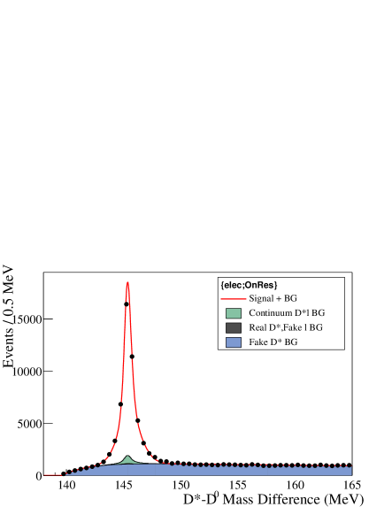
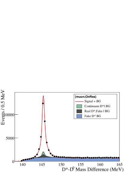
Figure 1: ${\rm\Delta}M$ distribution for events passing all selection criteria: $D^{*+}e^{-}$ (left) and $D^{*+}\mu^{-}$ (right) candidates in on-resonance data. Points correspond to data, and the curve is the result of unbinned maximum likelihood fits to this signal sample, the fake-lepton control sample and the rescaled off-resonance events. The shaded distributions correspond to the continuum, fake-lepton, and combinatorial backgrounds described in the text. The correlated-lepton, the $\bar{B}\rightarrow D^{*+}\ell^{-}\bar{\nu_{\ell}}X$ and the uncorrelated backgrounds are included in the signal distribution.

The fraction of combinatoric events below the $D^{*+}$ peak is determined from a fit to the $\Delta M$ distribution in the region $0.138<{\Delta M}<0.165~{}{\rm GeV}/c^{2}$ (see Figure 1). In the fit, $D^{*+}$ events are described by the sum of two Gaussian functions while the shape of combinatoric events is described by the function $\left[1-\exp\left(-\frac{\Delta m-m_{\pi}}{c_{1}}\right)\right]\left(\frac{\Delta m}{m_{\pi}}\right)^{c_{2}}$, where the overall normalization, $c_{1}$, and $c_{2}$ are determined by the fit. The width of the $\Delta M$ distribution for signal events is dominated by the experimental resolution. In one third of events the $\pi_{\rm slow}$  track is reconstructed in the SVT and in the DCH; in the remainder, the track is reconstructed only in the SVT. As the resolution in the first sample is better, the two samples are fitted separately.

The $\Delta M$  distribution of a fake-lepton control sample is fitted simultaneously to determine the fake-lepton background. The control sample is obtained by selecting events with the kinematic cuts described above, except for the requirement that the candidate lepton fails a loose lepton selection criterion. Lepton identification efficiencies and hadron misidentification probabilities, estimated from data control samples of pure leptons and hadrons, are used to scale the number of peaking events in this hadron-substituted sample to the expected amount of fake-lepton background in the signal sample.

The continuum contribution is fitted from the off-resonance event sample and scaled according to the ratio between the on-resonance and off-resonance luminosities.

For each $D^{0}$ final state, the signal, fake-lepton and continuum samples are fitted simultaneously. The mean values, widths and the relative normalization of the two Gaussian functions describing the signal are common to the three data sets, while the parameters describing the shape of the combinatoric background are fitted independently to each data sample. Cuts on $\Delta M$ are then applied to reduce the amount of combinatorics in the subsequent stages of the analysis: $0.143<{\Delta M}<0.148~{}{\rm GeV}/c^{2}$ if the $\pi_{\rm slow}$  is reconstructed by the SVT alone, $0.144<{\Delta M}<0.147~{}{\rm GeV}/c^{2}$ otherwise.

The fraction of uncorrelated and $D^{**}$  events is determined by exploiting the decay kinematics. The angle between the $B^{0}$ and the pseudo-particle obtained by adding the $D^{*+}$ and the $\ell^{-}$ four-momenta is computed according to the following expression:

$$\cos{\theta_{B^{0},D^{*}\ell}}=\frac{-(M^{2}_{B^{0}}+M^{2}_{D^{*}\ell}-2E_{B^{0}}E_{D^{*}\ell})+M^{2}_{\rm miss}}{2p_{B^{0}}p_{D^{*}\ell}},$$ (1)

where $M_{\rm miss}$ is the invariant mass of all the other particles produced in association with the lepton and the $D^{*+}$ in the decay of the $B^{0}$. We compute $\cos{\theta_{B^{0},D^{*}\ell}}$ by fixing $M_{\rm miss}$ to zero, under the hypothesis that this is a true $\bar{B^{0}}\rightarrow D^{*+}\ell^{-}\bar{\nu_{\ell}}$ decay, for which only a neutrino is missing. Neglecting the broadening due to experimental resolution, the obvious constraint $-1<\cos{\theta_{B^{0},D^{*}\ell}}<1$ applies to signal events. Due to the production of additional particles, events from $D^{**}$ background have positive $M^{2}_{\rm miss}$ values and therefore produce large tails below -1 in $\cos{\theta_{B^{0},D^{*}\ell}}$ distribution, while uncorrelated background events preferentially populate the region with $\cos{\theta_{B^{0},D^{*}\ell}}>1$. This allows for the determination of the fraction of $D^{**}$, uncorrelated, and signal events in the sample, by means of a fit to the $\cos{\theta_{B^{0},D^{*}\ell}}$ distribution in data (see for instance Figure 2). The shapes of all components in the fit are determined from Monte Carlo simulation, while the number of events for each of the other background categories is determined from the fit to the $\Delta M$  distributions. The same procedure is applied to 18 independent samples, identified according to lepton flavors ($\times 2$), period of data acquisition ($\times 3$), $D^{0}$ decay mode ($\times 3$). The data sets are further split into bins of $\tilde{w}$ (defined in Section 4.1) in order to reduce the systematic error corresponding to variations in background composition and normalization with ${\tilde{w}}$. The resulting large statistical uncertainties are reduced by requiring that the fractions of uncorrelated and $D^{**}$ background with respect to the signal be the same for electrons and muons, and for all $D^{0}$  decay modes. The validity of these hypotheses is verified by Monte Carlo simulation. The distributions in $\cos{\theta_{B^{0},D^{*}\ell}}$ for the $\bar{B^{0}}\rightarrow D^{*+}e^{-}\bar{\nu_{e}},D^{0}\rightarrow{K^{-}\pi^{+}}$ and $\bar{B^{0}}\rightarrow D^{*+}\mu^{-}\bar{\nu_{\mu}},D^{0}\rightarrow{K^{-}\pi^{+}\pi^{0}}$ samples (integrated over $\tilde{w}$ ) are shown in Figure 2.

Only events with $|\cos{\theta_{B^{0},D^{*}\ell}}|<1.2$ are further analyzed. This selects a final sample of 55700 signal events for the measurement.

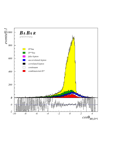
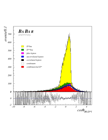
Figure 2: Distributions in $\cos{\theta_{B^{0},D^{*}\ell}}$ for the $\bar{B^{0}}\rightarrow D^{*+}e^{-}\bar{\nu_{e}},D^{0}\rightarrow{K^{-}\pi^{+}}$ (left) and $\bar{B^{0}}\rightarrow D^{*+}\mu^{-}\bar{\nu_{\mu}},D^{0}\rightarrow{K^{-}\pi^{+}\pi^{0}}$ samples (right). Points with error bars show the data. Shaded areas represent the Monte Carlo distributions. The fit determines the normalization of the Monte Carlo distributions. The tail to the left in the signal electron sample is due to bremsstrahlung. Below the histograms are shown the fractional deviations of the data from the fit results.

4 Determination of $|V_{cb}|$

4.1 Parametrization of the Decay Width

Assuming the connection between the various form factors provided by HQET, the expected number of signal events can be expressed as a function of $w$  by the relation

$$\frac{{\rm d}{\cal N}}{{\rm d}{w}}~{} = ~{}4~{}N_{\mathchar 28935\relax}~{}f_{00}~{}{\cal B}({D^{*+}}\rightarrow D^{0}{\pi^{+}_{\rm slow}})~{}{\cal B}(D^{0}\rightarrow K^{-}n\pi)~{}\epsilon({w})~{}\frac{{\rm d}{\cal B}}{{\rm d}{w}},$$

$$\frac{{\rm d}{\cal B}}{{\rm d}{w}}~{} = ~{}\frac{\displaystyle G^{2}_{F}}{\displaystyle 48\pi^{3}~{}\tau_{B^{0}}}M^{3}_{{D^{*+}}}(M_{B^{0}}-M_{{D^{*+}}})^{2}~{}\sqrt{{w}^{2}-1}~{}({w}+1)^{2}$$

$$\times \mid V_{cb}\mid^{2}~{}{\cal F}^{2}({w})\left[1+\frac{4{w}}{1+{w}}\frac{1-2{w}r+r^{2}}{(1-r)^{2}}\right].$$

The factor of 4 accounts for the fact that two B mesons are produced in each event, and that both electrons and muons are used; $N_{\mathchar 28935\relax}$ is the number of $\mathchar 28935\relax(4S)$ produced, $f_{00}$ is the fraction $\Gamma(\mathchar 28935\relax(4S)\rightarrow B^{0}\bar{B^{0}})/\Gamma(\mathchar 28935\relax(4S))$ , ${\cal B}({D^{*+}}\rightarrow D^{0}{\pi^{+}_{\rm slow}})$ is the branching fraction for the decay ${D^{*+}}\rightarrow D^{0}\pi^{+}$, ${\cal B}(D^{0}\rightarrow K^{-}n\pi)$ is the branching fraction for the decay of the $D^{0}$ to the final state considered, $\tau_{B^{0}}$ is the $B^{0}$  lifetime and $r$ is the ratio of meson masses, $r=M_{{D^{*+}}}/M_{B^{0}}$. The values employed for these parameters, as determined by independent measurements, are reported in Table 1.

Table 1: Values of inputs to the decay width calculation, as obtained from Ref.[18].

Parameter	Value
${\cal B}(D^{*+}\rightarrow D^{0}\pi^{+})$	$67.7\pm 0.5\%$
${\cal B}(D^{0}\rightarrow{K^{-}\pi^{+}})$	$3.80\pm 0.09\%$
${\cal B}(D^{0}\rightarrow{K^{-}\pi^{+}\pi^{+}\pi^{-}})$	$7.46\pm 0.31\%$
${\cal B}(D^{0}\rightarrow{K^{-}\pi^{+}\pi^{0}})$	$13.1\pm 0.9\%$
$\tau_{\overline{B}_{d}}$	$1.548\pm 0.018$ ps
$f_{+-}/f_{00}$	$1.055\pm 0.055$

The $w$-dependent reconstruction efficiency $\epsilon({w})$ is determined by means of the detailed detector simulation. The $w$ dependence of the form factor ${\cal F}$($w$) is unknown. Since only a small range of $w$ is allowed by phase space, a Taylor series expansion limited to second order has typically been used:

$${\cal F}({w})~{}=~{}{\cal F}(1)~{}(1+\rho^{2}_{\cal F}(1-{w})+c(1-{w})^{2}+{\cal O}(1-{w})^{3}).$$ (3)

Apart from ${\cal F}$(1), the theory does not predict the values of the higher order coefficients, which must be determined experimentally. The first measurements of $|V_{cb}|$  were performed assuming a linear expansion, i.e., setting $c=0$ ([7, 9, 10, 13]). However, the requirement of analyticity and positivity of the QCD functions describing the local currents leads to the prediction that $c$ should be positive and it should be related to the heavy meson radius $\rho^{2}_{\cal F}$(see [5]) by the relation:

$$c~{}=~{}0.66{{\rho^{2}_{\cal F}}}-0.11~{}.$$ (4)

Results employing this analyticity bound were obtained by the ALEPH, DELPHI and OPAL collaborations (see [11, 12, 14]). An improved parametrization based on the above consideration is proposed in [6], accounting for higher order terms and so reducing to $\pm 2$% the relative uncertainty on $|V_{cb}|$  due to the form factor parametrization. A new function ${\cal A}_{1}$($w$) is introduced in that calculation, connected to ${\cal F}$($w$) by the following relation:

$${\cal F}^{2}({w})~{} \times ~{}\left[1+\frac{4{w}}{1+{w}}\frac{1-2{w}r+r^{2}}{(1-r)^{2}}\right]~{}=~{}$$ (5)

$${\cal A}_{1}^{2}({w})~{} \times ~{}\left\{2\frac{1-2{w}r+r^{2}}{(1-r)^{2}}\left[1+\frac{{w}-1}{{w}+1}R_{1}({w})^{2}\right]+\left[1+\frac{{w}-1}{1-r}(1-R_{2}({w}))\right]^{2}\right\}$$

where $R_{1}$($w$) and $R_{2}$($w$) are ratios of axial and vector form factors also given in Ref. [6]. The following parametrization, depending only on a single unknown parameter $\rho^{2}_{{\cal A}_{1}}$, is proposed for ${\cal A}_{1}$($w$):

$${\cal A}_{1}({w})~{}=~{}{\cal A}_{1}(1)\times\left[1-8\rho^{2}_{{\cal A}_{1}}z+(53\rho^{2}_{{\cal A}_{1}}-15)z^{2}-(231\rho^{2}_{{\cal A}_{1}}-91)z^{3}\right]$$

with

$$z=\frac{\sqrt{{w}+1}-\sqrt{2}}{\sqrt{{w}+1}+\sqrt{2}}.$$

It should be noted that, in the limit ${w}\rightarrow 1$, ${{\cal A}_{1}}({w})\rightarrow{{\cal F}}({w})$, so that ${{\cal A}_{1}}(1)={{\cal F}}(1)$.

Monte Carlo events employed for this analysis were produced with a linear parametrization for ${\cal F}(w)$, while experimental data are fitted using expressions of Ref. [6].

Experimentally the variable $w$ can be expressed as:

$${w}=\frac{(M_{B^{0}}^{2}+M_{{D^{*+}}}^{2}-q^{2})}{(2M_{B^{0}}M_{{D^{*+}}})}$$

where $q^{2}\equiv(p_{B^{0}}-p_{{D^{*+}}})^{2}$. The magnitude of the $B^{0}$ momentum is known; its direction is obtained from Equation 1 with an azimuthal ambiguity about the direction of the ${D^{*+}}\ell^{-}$ pair. The two extreme solutions corresponding to the minimal and maximal angles between the $B^{0}$ and the $D^{*+}$ are used to define the quantity

$$\tilde{{w}}\equiv\frac{{w}_{\rm min}+{w}_{\rm max}}{2}.$$ (6)

The simulation shows that $\tilde{w}$ is a good estimator of $w$, with a resolution $\sigma(\tilde{{w}}-{w})\sim 0.02$, corresponding to about 4% of the full physical range.

4.2 Fit Method

Data and Monte Carlo simulated events are collected in ten equal-size $\tilde{w}$ bins. A few events, which, due to resolution, have ${\tilde{w}}>{w}_{\rm max}=1.503$ are discarded. A least-squares fit is then performed comparing the number of events observed in each bin to the sum of signal and background events. The number of background events in each bin is determined as explained above and is fixed in the fit. The signal contribution is obtained at each step in the minimization procedure by properly weighting each generated event surviving the selection. The $\chi^{2}$ is:

$$\chi^{2}=\sum_{i=1}^{10}\frac{(N^{i}_{\rm data}-N^{i}_{\rm bck}-\sum_{j=1}^{N^{i}_{\rm MC}}W_{j})^{2}}{N^{i}_{\rm data}+\sigma^{2}_{\rm bck}+\sum_{j=1}^{N^{i}_{\rm MC}}W_{j}^{2}},$$ (7)

where the index $i$ runs over the ten $\tilde{w}$ bins; $N^{i}_{\rm data(MC)}$ is the number of data (signal Monte Carlo) events found in the $i^{th}$ bin; $N^{i}_{\rm bck}$, $\sigma^{i}_{\rm bck}$ are the numbers of background events and their errors. The weight for each Monte Carlo event is computed as the product of three terms

$$W_{j}=W^{\cal L}\times W^{\epsilon}_{j}\times W^{theo}_{j},$$ (8)

where

• $W^{\cal L}$ is an overall fixed scale factor, that accounts for the relative luminosity of data and signal Monte Carlo events, for the difference in the actual branching fractions relevant to this analysis , and any possible overall efficiency scale factor.

• $W^{\epsilon}_{i}$ accounts for the efficiency correction, computed event per event as the ratio of the efficiency in the real data and in the Monte Carlo. It accounts for differences in tracking, particle identification, $\pi^{0}$ reconstruction, and depends on the three-momenta of the lepton, the soft pion and of all the particles from the $D^{0}$ decay. It remains unchanged at all steps of the minimization. (If the Monte Carlo simulation were perfectly tuned, this factor would be identically one). It should be noted that only the factor due to the slow pion tracking efficiency introduces a net dependence of this term on ${\tilde{w}}$.

• $W_{i}^{theo}=f_{\rm theo}({w};\rho^{2},|V_{cb}|)/f_{\rm MC}({w};\rho^{2}_{\rm MC},|V_{cb}|_{\rm MC})$ is the term accounting for the theoretical function describing the decay. It depends on the parameters to be determined (${\cal A}_{1}(1)|V_{cb}|$ and $\rho^{2}_{{\cal A}_{1}}$) and varies for each step of the minimization.

Here the function $f_{\rm theo}$ corresponds to the expressions in Equations 3 and 5, while the function used to generate Monte Carlo events, $f_{MC}$, contains a simpler, linear parametrization of the form factor dependence on ${w}$.

The value of the branching ratio is then computed by integrating the differential expression in Equation 3.

The fit has been performed as a blind analysis, i.e., the values of ${\cal A}_{1}(1)|V_{cb}|$ and $\rho^{2}_{{\cal A}_{1}}$ were hidden until the study of the systematic errors was completed and all consistency checks were performed.

4.3 Fit Results

The fit is performed separately for each data set, providing 18 statistically independent determinations of ${\cal A}_{1}(1)|V_{cb}|$ and of $\rho^{2}_{{\cal A}_{1}}$. The results are reported in Table 2. In the same Table, the branching fraction, as obtained by integrating the differential decay width, is also shown. The agreement between the data and the fit function is good. The distribution of the $\chi^{2}$ probabilities is uniform. The measured $w$ distributions are shown in Figure 3, where the three distributions for the $D^{0}$ decay modes are summed.

It should be noted that, because the statistical errors are small, the measurements are dominated by the systematic errors, which introduce considerable correlations among the samples. For this reason, first the systematic error is discussed, and then the average is presented.

Table 2: Fit results and the branching ratio ${\cal B}(\mbox{$\bar{B^{0}}\rightarrow D^{*+}\ell^{-}\bar{\nu_{\ell}}$})$ , for sub-samples defined by $D^{0}$ decay mode, lepton species, and year of data taking. The third columns shows the statistical correlation between ${\cal A}_{1}(1)|V_{cb}|$ and $\rho^{2}_{{\cal A}_{1}}$.

	$D^{0}$/lepton	${{\cal A}_{1}(1)|V_{cb}|}\times 10^{3}$	$\rho^{2}_{{\cal A}_{1}}$	Corrstat	${\cal B}$ $\%$	P($\chi^{2}$) $\%$
	$K\pi$/e	34.69$\pm$0.95	1.284$\pm$ 0.083	91$\%$	4.72$\pm$ 0.11	03.1
	$K\pi\pi\pi$/e	35.68$\pm$1.42	1.452$\pm$ 0.106	93$\%$	4.55$\pm$ 0.16	98.4
2000	$K\pi\pi^{0}$/e	32.36$\pm$1.17	1.241$\pm$ 0.109	93$\%$	4.21$\pm$ 0.12	20.7
	$K\pi$/$\mu$	33.00$\pm$0.99	1.145$\pm$ 0.097	92$\%$	4.61$\pm$ 0.11	21.6
	$K\pi\pi\pi$/$\mu$	33.51$\pm$1.48	1.410$\pm$ 0.127	93$\%$	4.11$\pm$ 0.15	26.0
	$K\pi\pi^{0}$/$\mu$	32.75$\pm$1.20	1.235$\pm$ 0.111	93$\%$	4.32$\pm$ 0.13	83.1
	$K\pi$/e	34.92$\pm$0.73	1.237$\pm$ 0.063	92$\%$	4.91$\pm$ 0.08	06.8
	$K\pi\pi\pi$/e	35.06$\pm$1.08	1.357$\pm$ 0.085	93$\%$	4.63$\pm$ 0.12	45.6
2001	$K\pi\pi^{0}$/e	33.68$\pm$0.89	1.190$\pm$ 0.081	93$\%$	4.69$\pm$ 0.09	70.1
	$K\pi$/$\mu$	34.35$\pm$0.78	1.242$\pm$ 0.070	92$\%$	4.74$\pm$ 0.09	25.6
	$K\pi\pi\pi$/$\mu$	34.83$\pm$1.16	1.407$\pm$ 0.092	93$\%$	4.45$\pm$ 0.13	41.8
	$K\pi\pi^{0}$/$\mu$	33.69$\pm$0.96	1.191$\pm$ 0.088	93$\%$	4.69$\pm$ 0.10	72.0
	$K\pi$/e	33.75$\pm$0.89	1.212$\pm$ 0.082	92$\%$	4.65$\pm$ 0.10	68.8
	$K\pi\pi\pi$/e	33.89$\pm$1.32	1.409$\pm$ 0.105	93$\%$	4.21$\pm$ 0.14	73.2
2002	$K\pi\pi^{0}$/e	35.41$\pm$1.06	1.364$\pm$ 0.085	92$\%$	4.71$\pm$ 0.12	93.3
	$K\pi$/$\mu$	32.71$\pm$1.06	1.034$\pm$ 0.107	93$\%$	4.81$\pm$ 0.12	37.6
	$K\pi\pi\pi$/$\mu$	33.84$\pm$1.52	1.323$\pm$ 0.129	93$\%$	4.40$\pm$ 0.17	45.6
	$K\pi\pi^{0}$/$\mu$	35.52$\pm$1.24	1.406$\pm$ 0.101	91$\%$	4.63$\pm$ 0.14	42.9

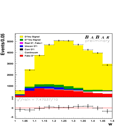
Figure 3: The experimental distribution of $w$ compared to fit results separately for electrons (left) and muons (right). The plots from all the different $D^{0}$ decay modes and years of data taking are summed together. The points are the data and the histograms are the results of the fit to the sum of the signal and the different sources of background. The fit residuals are also shown below.

4.4 Systematic Errors and Consistency Checks

The individual sources of systematic errors are reported in Table 4 and are described in detail below. They can be grouped as

• Factors affecting the overall normalization (see Equation 3): Each of these factors is varied by its uncertainty, and the resulting variation in the parameters is added to the systematic error. The uncertainties on $N_{\mathchar 28935\relax}$, $f_{00}$, $\tau_{B^{0}}$ and ${\cal B}({D^{*+}})$ are completely correlated for all the samples. The uncertainties on the $D^{0}$ branching fractions depend on the decay mode and are only partially correlated [18].

• Experimental uncertainties in the efficiency: These include track reconstruction, lepton and kaon identification, $\pi^{0}$ selection, vertex reconstruction and the cut on the Dalitz plot for the $K^{-}\pi^{+}\pi^{0}$ mode.
  For high-momentum tracks, the tracking efficiency is determined comparing the independent information from the SVT and DCH. This approach results in $\pm 0.8\%$ systematic uncertainty in the reconstruction efficiency for each track; the errors from each track are added linearly (i.e., the error on the branching fraction is $N$ times the single track error, where $N$ is the total number of tracks employed, including the lepton). Most of the $\pi_{\rm slow}$ do not reach the DCH, and are reconstructed in the SVT alone. The efficiency for these low-momentum tracks is computed from the angular distribution of the $\pi_{\rm slow}$ in the $D^{*+}$ rest frame. To evaluate this, a large set of ${D^{*+}}\rightarrow D^{0}{\pi^{+}_{\rm slow}}$, $D^{0}\rightarrow{K^{-}\pi^{+}}$ decays is selected from generic hadronic events. For fixed values of the $D^{*+}$  momentum, the observed angular distribution is compared to the one predicted for the decay of a vector meson to two pseudoscalar mesons, and the deviation from the expected shape is attributed to the inefficiency of track reconstruction. This inefficiency is parametrized as a function of the particle momentum in the laboratory frame. The values of the parameters describing the efficiency are computed in different bins of the polar angle of the track, both in the data and in the simulation. The systematic error is computed by varying each parameter of the efficiency function by its uncertainty, including correlations.

  The efficiencies and systematic errors for lepton and kaon identification and $\pi^{0}$ reconstruction are measured from control samples. The error on lepton identification is common to all samples (separately for each lepton type). Looser kaon identification criteria are imposed on $K^{-}\pi^{+}$ decays; the corresponding systematic error is therefore smaller than for $K^{-}\pi^{+}\pi^{+}\pi^{-}$ and $K^{-}\pi^{+}\pi^{0}$ decays.
  The systematic errors due to the cuts on the vertex probability and on the Dalitz plot are evaluated by varying these cuts.
  The efficiency corrections in data and in Monte Carlo simulation are largely independent of ${\tilde{w}}$, and therefore the value of $\rho^{2}_{{\cal A}_{1}}$ is scarcely affected, while a substantial error is induced on ${\cal A}_{1}(1)|V_{cb}|$  and branching fraction. Not surprisingly the most noticeable exception is the $\pi_{\rm slow}$ tracking efficiency correction, which affects both ${\cal A}_{1}(1)|V_{cb}|$ and $\rho^{2}_{{\cal A}_{1}}$.

  Table 3: Decay modes used in the Monte Carlo simulation of the $\bar{B}\rightarrow D^{*+}\ell^{-}\bar{\nu_{\ell}}X$. These branching fraction values are based mainly on theoretical estimates. The theoretical models adopted to generate these events are also listed. For the four-body $\bar{B}\rightarrow D^{*+}\ell^{-}\bar{\nu_{\ell}}\pi$ decays, the Goity and Roberts model (GR) [19] was used, while the Isgur and Scora model (ISGW2) [20] was adopted for the resonant $\bar{B}\rightarrow D^{**}\ell^{+}\nu_{\ell}$ decays.

  $B$ decay mode	${\cal B}(B)$	Model	$D^{**}$ decay	${\cal B}(D)$	Overall BR
  	$\times 10^{-2}$				$\times 10^{-4}$
  $B^{0}\rightarrow D^{*-}\pi^{0}\ell^{+}\nu_{\ell}$	0.10	GR	$-$	$-$	10.
  $B^{0}\rightarrow D^{-}_{1}\ell^{+}\nu_{\ell}$	0.56	ISGW2	$D^{-}_{1}\rightarrow D^{*-}\pi^{0}$	0.33	18.5
  $B^{0}\rightarrow D^{*-}_{1}\ell^{+}\nu_{\ell}$	0.37	ISGW2	$D^{*-}_{1}\rightarrow D^{*-}\pi^{0}$	0.33	12.2
  $B^{0}\rightarrow D^{*-}_{2}\ell^{+}\nu_{\ell}$	0.37	ISGW2	$D^{*-}_{2}\rightarrow D^{*-}\pi^{0}$	0.103	3.81
  $B^{0}\rightarrow D^{\prime-}\ell^{+}\nu_{\ell}$	0.02	ISGW2	$D^{\prime-}\rightarrow D^{*-}\pi^{0}$	0.33	0.67
  $B^{0}\rightarrow D^{*\prime-}\ell^{+}\nu_{\ell}$	0.22	ISGW2	$D^{*\prime-}\rightarrow D^{*-}\pi^{0}$	0.17	3.74
  $B^{+}\rightarrow D^{*-}\pi^{+}\ell^{+}\nu_{\ell}$	0.20	GR	$-$	$-$	20.
  $B^{+}\rightarrow D^{0}_{1}\ell^{+}\nu_{\ell}$	0.56	ISGW2	$D^{0}_{1}\rightarrow D^{*-}\pi^{+}$	0.67	37.5
  $B^{+}\rightarrow D^{*0}_{1}\ell^{+}\nu_{\ell}$	0.37	ISGW2	$D^{*0}_{1}\rightarrow D^{*-}\pi^{+}$	0.67	24.8
  $B^{+}\rightarrow D^{*0}_{2}\ell^{+}\nu_{\ell}$	0.37	ISGW2	$D^{*0}_{2}\rightarrow D^{*-}\pi^{+}$	0.21	7.78
  $B^{+}\rightarrow D^{\prime 0}\ell^{+}\nu_{\ell}$	0.02	ISGW2	$D^{\prime 0}\rightarrow D^{*-}\pi^{+}$	0.67	1.32
  $B^{+}\rightarrow D^{*\prime 0}\ell^{+}\nu_{\ell}$	0.22	ISGW2	$D^{*\prime 0}\rightarrow D^{*-}\pi^{+}$	0.33	7.26

• Background subtraction: The fraction of background events is determined in data for each $\tilde{w}$ bin as described above. This procedure considerably reduces the systematic error. The statistical error on the background is automatically accounted for by the fit (see Equation 7). A residual model dependence is considered for the $D^{**}$ background. Including narrow, wide and non-resonant ${D^{*+}}\pi$ states, a total of twelve modes (for $B^{0}$ and $B^{+}$ semileptonic decays) is considered. The $D^{**}$ background is computed assuming the branching fractions reported in Table 3. In order to estimate the systematic error due to the uncertainty in the shape of the $D^{**}$ background, the $\cos{\theta_{B^{0},D^{*}\ell}}$ fits in the different $w$ bins are performed considering only one decay mode a time, and the corresponding values of $|V_{cb}|$ and of $\rho^{2}_{{\cal A}_{1}}$are then determined again. The systematic error is then computed as half the difference between the maximum and minimum values of the parameters obtained from this study.
  To test whether the background from uncorrelated events is properly handled, the cut on $\cos\theta_{D^{*}\ell}<0$ is removed and the study is repeated. This results in an increase of the uncorrelated background by a factor of about 2 in the full $\cos{\theta_{B^{0},D^{*}\ell}}$ range, and by 30% in the signal region. No appreciable change in the fit result is observed. As an alternative, the fraction of uncorrelated events is determined by counting the events in the rejected region $\cos\theta_{D^{*}\ell}>0$ and propagating this number to the complementary region using the Monte Carlo. The fraction obtained is then fixed in the $\cos{\theta_{B^{0},D^{*}\ell}}$ fit, which is used to determine the fraction of $D^{**}$ and signal events only. Once again, no appreciable change in the result is observed.
  Finally, the hypothesis that the ratio of the amount of $D^{**}$ and uncorrelated background over the signal be the same for all $D^{*+}$ decay modes is checked with the simulation. While the test is satisfactory for the uncorrelated background, a slight discrepancy is observed for $D^{**}$ events. For $K^{-}\pi^{+}\pi^{+}\pi^{-}$ decay the fitted fraction is higher by 30% than for the other modes. The effect is the same for electron and muon events and does not depend on ${\tilde{w}}$. Therefore the $\tilde{w}$ fit is repeated by increasing the $D^{**}$ amount in the $K^{-}\pi^{+}\pi^{+}\pi^{-}$ sample and decreasing it correspondingly in the $K^{-}\pi^{+}$ and $K^{-}\pi^{+}\pi^{0}$ . The difference in the result is propagated as systematic error.

• Theoretical uncertainties: A considerable fraction of the allowed phase-space is removed by the lower limit on the lepton momentum. This induces a model-dependence in the computation of the branching fraction. The lepton spectrum is determined partly by the fitted shape of the Isgur-Wise function, and partly by the angular profile of the decay, which is governed by the parameters $R_{1}$ and $R_{2}$ defined above. Even with perfect acceptance, the uncertainty on $R_{1}$ and $R_{2}$ directly affects $\rho^{2}_{{\cal A}_{1}}$ and ${\cal A}_{1}(1)|V_{cb}|$, because these parameters enter in the fit function. The values of these parameters determined by the CLEO collaboration [21] are used in this analysis. The systematic error is taken as the observed variation of ${\cal A}_{1}(1)|V_{cb}|$, $\rho^{2}_{{\cal A}_{1}}$ and of ${\cal B}(\mbox{$\bar{B^{0}}\rightarrow D^{*+}\ell^{-}\bar{\nu_{\ell}}$})$, when $R_{1}$ and $R_{2}$ are floated by their uncertainties, accounting for their correlation.

• Fit method: The fit procedure is validated using an independent sample of Monte Carlo simulated events, of the same size as the data, and following the procedure described above, using however a linear extrapolation for the Isgur-Wise function. The fitted values of $\rho^{2}_{{\cal A}_{1}}$ and ${\cal A}_{1}(1)|V_{cb}|$ are consistent within their statistical errors with the input values. The statistical error on this test is added to the systematic error. In addition, to test that the fit method does not bias the result, a set of 500 toy experiments are performed, in which random events are generated with realistic efficiency and resolution. Each toy experiment has the same sample size for data and Monte Carlo as in the actual measurement. Within errors, no difference is observed between the average of the fitted parameters and their generated values. Also, it is observed that the pull width is consistent with one.

Table 4: Summary of all statistical and systematic errors.

error contribution	$\delta{{\cal A}_{1}(1)|V_{cb}|}/{{\cal A}_{1}(1)|V_{cb}|}$ ($\%$)	$\delta$$\rho^{2}_{{\cal A}_{1}}$	$\delta{\cal B}/{\cal B}$ ($\%$)
statistics (data and MC)	0.7	0.02	0.8
particle identification	0.5	-	0.9
$\pi_{\rm slow}$ efficiency	1.3	0.02	1.9
tracking $\&$ $\pi^{0}$ efficiency	1.3	-	2.7
$D^{*+}\ell^{-}$ vertexing efficiency	0.5	-	1.0
$w$  fit method	0.6	0.02	1.2
$\cos{\theta_{B^{0},D^{*}\ell}}$ $\chi^{2}$ fit binning	0.5	-	1.0
$D^{**}$ background composition	1.8	0.06	2.0
total number of $B$ produced	0.6	-	1.1
$\mathchar 28935\relax{(4S)}$ rest frame $B$ momentum	0.3	-	0.7
$R_{1}(1)$ and $R_{2}(1)$	1.8	0.27	1.8
total systematic error	3.4	0.28	5.0
$\tau_{B^{0}}$	0.6	-	-
${\cal B}(D^{0})$	1.1	-	2.0
${\cal B}(D^{*+}\rightarrow D^{0}\pi^{+})$	0.4	-	0.7
${\cal B}(\mathchar 28935\relax{(4S)}\rightarrow B^{0}{\kern-1.60004pt\kern 1.79993pt\overline{\kern-1.79993ptB}{}^{0}})$	1.3	-	2.7
total systematic error	1.8	-	3.5

4.5 Results

The results from all subsamples are combined by using the COMBOS package [22], taking into account the correlations between the samples. COMBOS was originally developed by the LEP-B-Oscillation working group to combine the results of $\Delta M_{d}$ from different experiments, and was then adapted by the LEP-V_cb working group to compute the world average for $|V_{cb}|$, $\rho^{2}_{{\cal A}_{1}}$ and ${\cal B}(\mbox{$\bar{B^{0}}\rightarrow D^{*+}\ell^{-}\bar{\nu_{\ell}}$})$. Besides computing averages, errors, and confidence levels, COMBOS also provides a breakdown of the single error sources, which is reported in Table 4.

All the parameters affecting the normalization are treated as fully correlated. The errors on the branching fractions of the $D^{0}$ to each final state are fully correlated for each state, but, at present, the correlations among different decay modes are neglected. The systematic errors on particle identification are considered as fully correlated among data taking periods. The error on tracking is determined by systematic effects common to all years and therefore is considered as fully correlated among all the samples. In contrast the error on $\pi_{\rm slow}$ tracking efficiency is still dominated by the statistical uncertainty from the control samples; therefore it is completely correlated for samples collected in the same year of data acquisition, but uncorrelated for different years. Model errors are common to all data sets.
The mean values are obtained by first averaging results for different running periods, and then computing the average result for the three years. The confidence level of the ${\cal A}_{1}(1)|V_{cb}|$ and $\rho^{2}_{{\cal A}_{1}}$ average values is 30%. The results are reported in Table 5.

Table 5: Fit results for the three running periods.

year	${{\cal A}_{1}(1)|V_{cb}|}\times 10^{3}$	$\rho^{2}_{{\cal A}_{1}}$
2000	33.60$\pm$0.46$\pm$1.33	1.23$\pm$0.04$\pm$0.28
2001	34.63$\pm$0.36$\pm$1.44	1.25$\pm$0.03$\pm$0.28
2002	34.73$\pm$0.45$\pm$1.39	1.31$\pm$0.04$\pm$0.28
Total Average	34.03$\pm$0.24$\pm$1.31	1.23$\pm$0.02$\pm$0.28

For the sum of all 18 data subsamples the following result is obtained:

$${${\cal A}_{1}(1)|V_{cb}|$} = (34.03\pm 0.24\pm 1.31)\times 10^{-3},$$ (9)

$$\rho^{2}_{{\cal A}_{1}} = 1.23\pm 0.02\pm 0.28,$$ (10)

$${\cal B}(\mbox{$\bar{B^{0}}\rightarrow D^{*+}\ell^{-}\bar{\nu_{\ell}}$}) = (4.68\pm 0.03\pm 0.29)~{}\%,$$ (11)

where the first error is statistical and the second is systematic. The statistical correlation between ${\cal A}_{1}(1)|V_{cb}|$and $\rho^{2}_{{\cal A}_{1}}$is 92$\%$.

5 Conclusions

A sample of 55,700 signal events from the decay process $\bar{B^{0}}\rightarrow D^{*+}\ell^{-}\bar{\nu_{\ell}}$ is selected from a set of $86\times 10^{6}$ $\mathchar 28935\relax{(4S)}\rightarrow B\kern 1.79993pt\overline{\kern-1.79993ptB}{}$ decays collected by the BABAR detector. The product of $|V_{cb}|$ and the form factor at zero recoil, ${\cal F}(1)={\cal A}_{1}(1)$, is measured, as well as the derivative of the form factor, $\rho^{2}_{{\cal A}_{1}}$, again at zero recoil. The integrated branching fraction is also computed. These results are in agreement with those obtained by Belle [8] and with the LEP average [18], but differ by more than two standard deviations from the CLEO result [9]. Using the value ${\cal A}(1)=0.913^{+0.030}_{-0.035}$ reported in [4], based on a lattice QCD calculation, the value:

$$|V_{cb}| = (37.27\pm 0.26\mathrm{(stat.)}\pm 1.43\mathrm{(syst.)}^{+1.48}_{-1.23}\mathrm{(th.)})\times 10^{-3}$$ (12)

is then computed.

From the measurements of the hadronic mass moments and decay rate for the inclusive semileptonic $B$ decays BABAR has obtained another determination of $|V_{cb}|$ [23]. The preliminary result is:

$$|V_{cb}| = (42.1\pm 1.04\mathrm{(exp.)}\pm 0.72\mathrm{(th.)})\times 10^{-3}$$ (13)

Both the experimental and theoretical errors are independent. By interpreting the theoretical errors as $\pm 68\%$ confidence interval, the two values differ by 2.0 standard deviations.

6 Acknowledgments

We are grateful for the extraordinary contributions of our PEP-II colleagues in achieving the excellent luminosity and machine conditions that have made this work possible. The success of this project also relies critically on the expertise and dedication of the computing organizations that support BABAR. The collaborating institutions wish to thank SLAC for its support and the kind hospitality extended to them. This work is supported by the US Department of Energy and National Science Foundation, the Natural Sciences and Engineering Research Council (Canada), Institute of High Energy Physics (China), the Commissariat à l’Energie Atomique and Institut National de Physique Nucléaire et de Physique des Particules (France), the Bundesministerium für Bildung und Forschung and Deutsche Forschungsgemeinschaft (Germany), the Istituto Nazionale di Fisica Nucleare (Italy), the Foundation for Fundamental Research on Matter (The Netherlands), the Research Council of Norway, the Ministry of Science and Technology of the Russian Federation, and the Particle Physics and Astronomy Research Council (United Kingdom). Individuals have received support from the A. P. Sloan Foundation, the Research Corporation, and the Alexander von Humboldt Foundation.

References

- [1] M. A. Shifman and M. B. Voloshin, Sov. J. Nucl. Phys. 47 (1988) 511; N. Isgur and M. Wise, Phys. Lett. 237 (1990) 527; A. F. Falk, H. Georgi, B. Grinstein and M. B. Wise, Nucl. Phys. B 343 (1990) 1; M. Neubert, Phys. Lett. B 264 (1991) 455; M. Neubert, Phys. Lett. B 338 (1994) 84.
- [2] A. F. Falk, M. Neubert, Phys. Rev. D 47(1993) 2965 and 2982; T. Mannel, Phys. Rev. D 50 (1994) 428; M. A. Shifman, N. G. Uraltsev and M. B. Voloshin, Phys. Rev. D 51 (1995) 2217.
- [3] A. Czarnecki, Phys. Rev. Lett. 76 (1996) 4126.
- [4] S. Hashimoto et al., Phys. Rev. D 66, 014503 (2002).
- [5] I. Caprini, M. Neubert, Phys. Lett. B 380 (1996) 376.
- [6] I. Caprini, L. Lellouch, M. Neubert, Nucl. Phys. B 530 (1998) 153;C. G. Boyd, B. Grinstein, R. F. Lebed, Phys. Rev. D 56 (1997) 6895.
- [7] H. Albrecht et al. (ARGUS Coll.), Z. Phys. C 57 (1993) 533.
- [8] A. Abe et al. (BELLE Coll.), Phys. Lett. B 526 (2002) 258.
- [9] B. Barish et al. (CLEO Coll.), Phys. Rev. D 51 (1995) 1014;R.A. Briere et al. (CLEO Coll.), Phys. Rev. Lett 89 (2002) 081803;N.E. Adam et al. (CLEO Coll.), Phys. Rev. D 67 (2003) 032001;
- [10] B. Buskulic et al. (ALEPH Coll.), Phys. Lett. B 359 (1995) 236.
- [11] B. Buskulic et al. (ALEPH Coll.), Phys. Lett. B 395 (1997) 373.
- [12] P. Abreu et al. (DELPHI Coll.) P. Abreu et al. (DELPHI Coll.), Phys. Lett. B 510 (2001) 55.
- [13] P. Abreu et al. (DELPHI Coll.), Z. Phys. C 71 (1996) 539.
- [14] K. Ackerstaff et al. (OPAL Coll.), Phys. Lett. B 395 (1997) 128.
- [15] ‘PEP-II: An Asymmetric factory’, Conceptual Design Report, SLAC-418, LBL-5379 (1993).
- [16] B. Aubert et al. (BABAR Coll.) Nucl. Instrum. Methods A 479 (2002) 1-116.
- [17] P. L. Frabetti et al. (E687 Coll.), Phys. Lett. B 331 (1994) 217.
- [18] K. Hagiwara et al., Phys. Rev. D 66, (2002) 010001.
- [19] J. L. Goity and W. Roberts, Phys. Rev. D 51 (1995) 3459
- [20] D. Scora and N. Isgur, Phys. Rev. D 52 (1995) 2783.
- [21] J. Duboscq et al. (CLEO Coll.), Phys. Rev. Lett. 76 (1996) 3898.
- [22] O. Schneider and H. Seywerd, cern-ep-2001-050 (http://lepbosc.web.cern.ch/LEPBOSC/combos/).
- [23] B. Aubert et al. (BABAR Coll.), BABAR-CONF-03-013, hep-ex/0307046, Jul 2003