Observation of Atmospheric Neutrino Oscillations
in Soudan 2

Abstract

The effects of oscillations of atmospheric $\nu_{\mu}$ are observed in the 5.90 fiducial kiloton-year exposure of the Soudan 2 detector. An unbinned maximum likelihood analysis of the neutrino $L/E$ distribution has been carried out using the Feldman-Cousins prescription. The probability of the no oscillation hypothesis is $5.8\times 10^{-4}$. The 90% confidence allowed region in the $\sin^{2}2\theta,\Delta m^{2}$ plane is presented.

PACS numbers: 14.60.Lm, 14.60.Pq, 95.85.Ry

1 Introduction

The discovery of neutrino oscillations in both atmospheric and solar neutrinos and thus the establishment of neutrino mass has been one of the major advances in particle physics of the past decade. The evidence generally regarded as establishing neutrino oscillations was the observation by the Super-Kamiokande collaboration of a variation of the atmospheric neutrino event rate with zenith angle [1]. Solar neutrino oscillations have been confirmed by the SNO experiment’s measurement of the neutral current event rate [2] and the detection of the disappearance of reactor neutrinos by KamLAND [3]. The K2K experiment has provided supporting evidence for $\nu_{\mu}$ oscillations [4] but there has been no detailed confirmation of the Super-K effect in atmospheric neutrinos. Observations of a deficit of atmospheric $\nu_{\mu}$ have been published by this experiment [5], and by Kamiokande [6], IMB [7] and MACRO [8]. The analysis reported here is the first independent confirmation of atmospheric neutrino oscillations using fully reconstructed neutrino interactions and covering the complete range of zenith angles.

The data used are from the 5.90 fiducial kton-year exposure of the Soudan 2 detector. Soudan 2 was originally designed to study proton decay and thus has excellent resolution and pattern recognition properties in the visible energy region around 1 GeV where the peak in the atmospheric neutrino event rate occurs. Although the exposure of the experiment is less than that of Super-K, the full event reconstruction, and thus good energy and direction resolution for the incident neutrino, compensates to some extent for the smaller number of events.

The data are analyzed using an unbinned likelihood method based on the Feldman-Cousins prescription [9]. The probability of the no oscillation hypothesis is $5.8\times 10^{-4}$. The 90% confidence allowed region in the $\sin^{2}2\theta,\Delta m^{2}$ plane is determined and is consistent with that published by Super-K.

2 Detector and Data Exposure

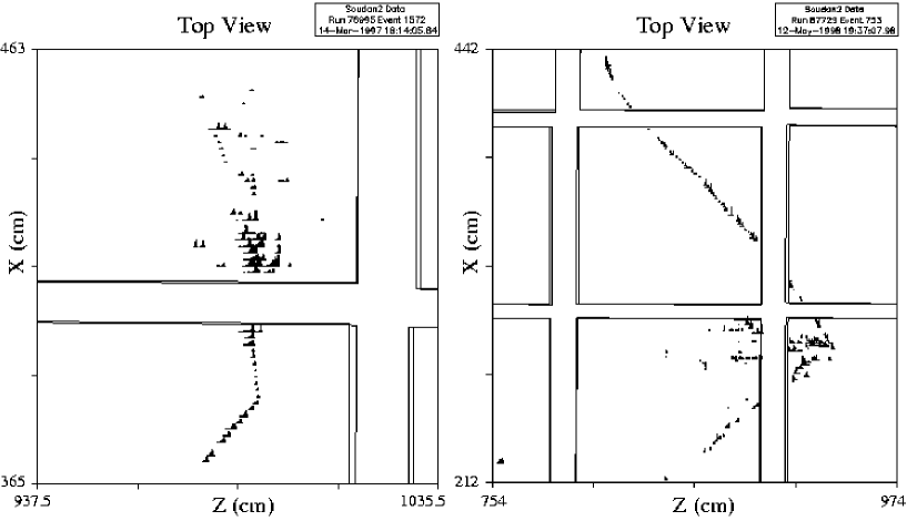
Figure 1: Two neutrino interactions in Soudan 2. The event on the left is a quasi-elastic $\nu_{e}$ interaction producing a proton and an electron. The electron travels about one radiation length before showering. The proton is easily recognizable by its heavy ionization (large symbols) and its lack of Coulomb scattering. The event on the right has a long non-interacting muon track, which shows typical Coulomb scattering, and a hadronic shower at the vertex. The shower contains a charged pion and at least two electromagnetic showers.

Soudan 2 is a 963 metric ton (770 tons fiducial) iron tracking calorimeter with a honeycomb geometry which operates as a time projection chamber. The detector is located at a depth of 2070 meters–water–equivalent on the 27th level of the Soudan Underground Mine State Park in northern Minnesota. The calorimeter started data taking in April 1989 and ceased operation in June 2001 by which time a total exposure of 7.36 kton-years, corresponding to a fiducial exposure of 5.90 kton-years, had been obtained.

The calorimeter’s active elements are 1 m long, 1.5 cm diameter hytrel plastic drift tubes filled with an argon-CO₂ gas mixture. The tubes are encased in a honeycomb matrix of 1.6 mm thick corrugated steel plates. Electrons deposited in the gas by the passage of charged particles drifted to the tube ends under the influence of an electric field. At the tube ends the electrons were amplified by vertical anode wires which read out a column of tubes. A horizontal cathode strip read out the induced charge and the third coordinate was provided by the drift time. The ionization deposited was measured by the anode pulse height. The steel sheets are stacked to form 1$\times$1$\times$2.5 m³, 4.3 ton modules from which the calorimeter was assembled in building-block fashion. More details of the construction of the detector and its properties can be found in Ref. [10].

Surrounding the tracking calorimeter on all sides but mounted on the cavern walls, well separated from the outer surfaces of the calorimeter, is a 1700 m² active shield array of two or three layers of proportional tubes [11]. The shield tagged the presence of cosmic ray muons in time with events in the main calorimeter and thus identified background events, either produced directly by the muons or initiated by secondary particles coming from muon interactions in the rock walls of the cavern.

Calibration of the calorimeter response was carried out at the Rutherford Laboratory ISIS spallation neutron facility using test beams of pions, electrons, muons, and protons [12]. Spatial resolutions for track reconstruction and for vertex placement in anode, cathode, and drift time coordinates are of the same scale as the drift tube radii, $\approx$ 0.7 cm.

Soudan 2 has several advantages over water Cherenkov detectors. Images approaching the quality of bubble chamber events are obtained. Ionizing particles having non-relativistic as well as relativistic momenta are detected via their energy loss in the gas. Protons are readily distinguished from $\pi^{\pm}$ and $\mu^{\pm}$ tracks by their ionization and lack of multiple Coulomb scattering. Muons from $\nu_{\mu}$ charged current (CC) reactions are prompt tracks without secondary scatters. Prompt e^± showers from $\nu_{e}$ CC reactions are distinguished from photon showers on the basis of their proximity to the primary vertex. Since Soudan 2 has no magnetic field and thus only limited charge identification, $\nu$ and $\bar{\nu}$ reactions are not separated.

Two examples of the event definition provided by the detector are shown in Fig. 1. The event on the left is a quasi-elastic $\nu_{e}$ interaction producing a short proton and an electron which travels approximately one radiation length before showering. The event on the right is an inelastic $\nu_{\mu}$ interaction. The long non-interacting muon track is accompanied by a hadronic shower, including a charged pion and at least two gamma showers.

The excellent imaging and particle identification offer good determination of the energy and direction of the incident neutrino and thus the path length from its production point in the atmosphere. Especially advantageous is the reconstruction of quasi-elastic reactions, where the recoil proton is observed with approximately 40% efficiency, and complicated multiprong topologies. The correlation of the outgoing lepton direction and energy with the incident neutrino direction and energy is poor at low energies. Improvements in the resolution of neutrino path length divided by energy, $L/E$ , by factors of 2 and 3 are readily obtained by reconstructing both the lepton and the hadronic final state.

3 Event Classes and Processing

3.1 Containment classes

Events are divided into two containment classes.

1. Events that are fully contained within the detector (FCE). Containment is defined by the requirement that no portion of the event approaches closer than 20 cm to the exterior of the detector and that no particle in the event could enter or escape the detector through the space between modules. The containment criterion limits high energy $\nu_{\mu}$ events to those with a muon of energy less than around 1 GeV.

2. Events that are partially contained, in which only the produced lepton exits the detector (PCE). These events recover a fraction of the high energy $\nu_{\mu}$ events rejected by the containment criterion. As the muon does not stop in the detector, its energy from range cannot be measured. Instead an estimate of the energy was obtained from the observed range, with a small added correction based on the amount of multiple scattering on the track. Monte Carlo (MC) studies showed that the effect of the poorer energy measurement on the $L/E$ resolution was small. Since the timing resolution of Soudan 2 is insufficient to determine the $\mu$ direction, a stopping, downward-going, cosmic ray muon could mimic an upward-going PCE having little or no hadronic vertex activity. Up-down asymmetric cuts on the exiting track and the event vertex properties are required to reduce this contamination to negligible proportions [13].

3.2 Veto Shield classes

Two classes of events are defined on the basis of the presence or absence of hits in the veto shield.

1. Quiet shield events. These events have no in-time hits in the veto shield except for those associated with the leaving lepton in PCEs. They are candidates for neutrino interactions but also contain a small background of events produced by cosmic ray muons. They will be called “qs-data” events.

2. Shield tagged events. Events initiated by the passage of a cosmic ray muon generally have in-time hits in the veto shield. The hits may be caused by the muon itself or by secondary charged particles from the interaction of the muon in the rock surrounding the detector. Secondary neutral particles can enter the detector and interact, mimicking neutrino interactions. Events flagged with in-time veto shield hits will be called “rock” events.

The average shield efficiency for detection of a minimum ionizing particle was measured to be 94%. Study of events with a single shield hit showed that the contamination of qs-data events by cosmic ray muons which pass through the shield and enter the detector is negligible. It was however possible for neutrons and gamma rays to enter the detector with no identifying shield hit when all of the charged particles associated with the production event in the rock passed outside the shield or were not detected due to shield inefficiency. These quiet shield rock events (called “qs-rock”) are a background to the neutrino sample. They may be statistically distinguished from neutrino events by the depth distribution of the interaction vertices, as described in Sect. 4.

3.3 Topology classes

The background from qs-rock events is significantly different in low and high multiplicity events and in low multiplicity electron and muon samples. The FCE data are thus further divided into topology classes.

1. Events with a single track-like particle with or without a recoil proton, called “tracks”. These are mostly quasi-elastic $\nu_{\mu}$ interactions and are assigned “$\mu$-flavor”.

2. Events with a single showering particle with or without a recoil proton called “showers”. These are mostly quasi-elastic $\nu_{e}$ interactions and are assigned “e-flavor”.

3. Events with multiple outgoing tracks and/or showers called “multiprongs”. These can be of either flavor. The flavor is assigned according to whether the highest energy secondary is a non-scattering track ($\mu$-flavor) or shower (e-flavor). A small fraction of multiprongs have no muon or electron candidate and are defined as neutral current, “NC”. A further small sample had no obvious flavor and are defined as ambiguous. The NC events are too few to provide constraints on the oscillation analysis but they and the ambiguous events are added into the event total, contributing to the flux normalization. Through the rest of the paper, unless otherwise specified, the heading NC includes both neutral current and ambiguous events.

3.4 High resolution sample

At low neutrino energies the correlation between the direction of the outgoing lepton and the incoming neutrino is poor. The ability of Soudan 2 to reconstruct the recoil proton from quasi-elastic interactions and the low energy particles from inelastic reactions gives a major improvement in the neutrino pointing and energy resolution. To take advantage of this, the events are finally divided into two samples depending on the $L/E$ resolution.

1. A high resolution “HiRes” sample:

   1. events with a single lepton of kinetic energy $>$600 MeV,

   2. events with a single lepton of kinetic energy $>$150 MeV with a reconstructed recoil proton,

   3. multiprong events with lepton kinetic energy $>$250 MeV, total visible momentum $>$450 MeV/$c$ and total visible energy $>$700 MeV,

   4. partially contained events.

   The mean neutrino pointing error for events in this sample is $33^{\circ}$ for $\nu_{\mu}$ FCE, $21^{\circ}$ for $\nu_{e}$ FCE and $14^{\circ}$ for $\nu_{\mu}$ PCE. This yields a mean error in $\log_{10}L/E$ of approximately 0.2.

2. A low resolution “LoRes” sample, comprising all other events.

3.5 Monte Carlo neutrino events

To avoid biases due to the scanning described in Sect. 3.6 and to provide a blind analysis, Monte Carlo events were inserted into the data stream as the data were taken. A Monte Carlo sample 6.1 times the expected data sample in this exposure, assuming no oscillations, was included. The Monte Carlo and data events were then processed simultaneously and identically through the analysis chain. The Monte Carlo representation of the detector and background noise was of sufficient quality that a human scanner could not distinguish between data and Monte Carlo events. The event generation was carried out using the NEUGEN package [14] and the particle transport using GHEISHA [15] and EGS [16]. The incident neutrino flux used in the generation of events was that provided by the Bartol group at the start of the experiment [17]. Later calculations of the neutrino flux were accommodated by weighting the generated events. The main analysis described below used the Bartol 96 flux [18]. A recent three-dimensional calculation of Battistoni et al. [19] has also been used. The variation in the flux during the solar cycle was taken into account using measured neutron monitor data for normalization [20]. The Monte Carlo events were superimposed on random triggers which represent the background noise in the detector, mostly low energy gammas from radioactive decays or electronic noise. This simulated the effect of random noise on the event recognition and reconstruction and the random vetoing of events (4.8%) due to noise in the veto shield.

3.6 Data processing

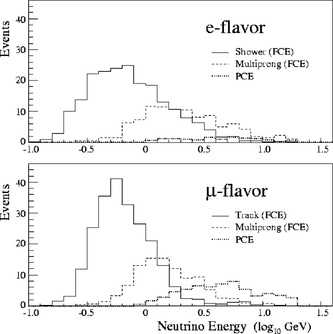
Figure 2: Unoscillated Monte Carlo neutrino energy distributions for the fully contained shower or track, fully contained multiprong and PCE classes. The top plot is for e-flavor events and the bottom plot for $\mu$-flavor events.

The detector trigger rate was approximately 0.5 Hz. About half of the triggered events were cosmic ray muons and half electronic noise or the sum of random low energy gamma radiation. The trigger required 7 anodes or 8 cathodes to have signals in any contiguous set of 16 multiplexed channels. The 50% efficiency thresholds are approximately 100 MeV for single electrons and 150 MeV kinetic energy for single muons.

The data, including the Monte Carlo events, were processed through the standard Soudan 2 reconstruction code to select possible contained and partially contained events. Approximately 0.1% of events were retained for further analysis. These events were double scanned to verify containment and remove remaining noise backgrounds. Surviving events were checked and assigned flavor by three independent physicist scans. Throughout this process qs-data, rock and MC events were treated identically, without their origin being known to the scanners. The classifications based on confinement, topology and resolution were also applied equally to the three data types.

Accepted events were reconstructed using an interactive graphics system. All recognizable tracks and showers in the event were individually measured yielding momenta and energies. Protons were identified by their high ionization and lack of Coulomb scattering. Finally the individual particle momenta and energies were added to form the incoming neutrino four-vector.

The topology classes provide a crude energy separation. The track and shower samples have a lower average neutrino energy than the multiprong sample and both are lower than the mean PCE energy. Histograms of the Monte Carlo generated neutrino energy, $E_{\nu}$, for the three classes are shown in Fig. 2 for the $\mu$-flavor and e-flavor events. Note that the contained single shower distribution extends to higher energies than the track sample because of the better containment of high energy showers.

The numbers of events analyzed are shown in Table 1. The oscillation analysis described in this paper imposed a minimum 300 MeV/$c$ cut on the lepton momentum for LoRes track and shower events and the total visible momentum for LoRes multiprong events. The numbers headed “Raw Events” in the table are those for the total event sample without this cut, the other numbers include the cut. The table shows that the rock background is concentrated in low energy events which are removed by the cut. The value of the cut was chosen to optimize the analysis sensitivity by reducing the background component while retaining the neutrino signal. The final two columns are the fitted number of qs-rock events and the number of neutrino events after subtraction of the qs-rock background as described in Sect. 4.1.1.

More details of the data sample and the analysis procedures are given in Ref. [21].

Event	Fla-	Raw Events			300 MeV/$c$ cut
Class	vor	qs-data	MC	rock	qs-data	MC	rock	qs-rock	neutrino
FCE HiRes	$\mu$	114	1149	73	114	1115.1	73	12.1$\pm$6.9	101.9$\pm$12.7
FCE HiRes	e	152	1070	69	152	1047.4	69	5.3$\pm$2.1	146.7$\pm$12.5
FCE LoRes	$\mu$	148	900	406	61	457.5	77	11.5$\pm$6.2	49.5$\pm$9.9
FCE LoRes	e	177	850	704	71	402.5	176	14.0$\pm$4.6	57.0$\pm$9.6
PCE	$\mu$	53	373	11	53	384.3	11	0.3$\pm$0.9	52.7$\pm$7.3
PCE	e	5	51	0	5	51.5	0	0.0$\pm$0.1	5.0$\pm$2.2
NC+ambig		46	246	190	32	165.7	110	7.6$\pm$6.7	24.4$\pm$8.8
Total		695	4639	1453	488	3624.0	516	50.8	437.2

Table 1: Event samples in the 5.90 fiducial kiloton-year exposure. The columns for raw events are the total numbers of events reconstructed in this experiment. The qs-data, MC and rock classes are defined in Sects. 3.2 and 3.5. The columns headed “ 300 MeV/$c$ cut ” give the event numbers used in the oscillation analysis described in this paper. The MC numbers in these columns have been weighted to convert from the Bartol 89 flux prediction to the Bartol 96 values. The qs-rock column gives the fitted number of background qs-rock events and the neutrino column is the number of neutrino qs-data events after subtraction of the qs-rock background as described in Sect. 4.1.1.

4 Evidence for $\nu_{\mu}$ flavor disappearance

The neutrino oscillation parameters were determined using an unbinned maximum likelihood analysis of the complete data set based upon the Feldman-Cousins procedure, as described in Sect. 5. However it is instructive first to examine subsets of the data to observe the effects of oscillations.

4.1 Flavor Ratio-of-Ratios

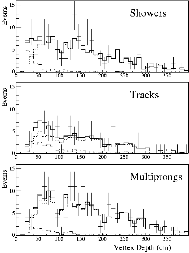
Figure 3: Depth distributions for shower (top), track (center), and multiprong events (bottom) after the 300 MeV/$c$ cut. The points with error bars are the qs-data events. The dashed histograms are the unoscillated Monte Carlo events. The dotted histograms are the rock events and the solid histograms are the sum of Monte Carlo and rock. The fraction of qs-rock is determined from a fit of the Monte Carlo plus rock events to the qs-data event distribution. The summed distribution is normalized to the qs-data events.

The first indication of neutrino oscillations in atmospheric neutrinos came from the measurement of the ratio-of-ratios, $R_{\nu}$ [6], defined here as

$$R_{\nu}=\frac{(\nu_{\mu}/\nu_{e})_{data}}{(\nu_{\mu}/\nu_{e})_{MC}}.$$ (1)

Two corrections, for qs-rock background and for flavor misidentification, are required to the raw numbers of qs-data $\mu$-flavor and e-flavor events.

4.1.1 Correction for qs-rock background

For the measurement of $R_{\nu}$, the number of qs-rock background events contained in the qs-data sample was estimated by fitting the depth distribution of the qs-data events to a sum of the MC and rock depth distributions. The extended maximum likelihood method of Ref. [22] was used, which allows for the finite statistics of the Monte Carlo and rock distributions. The depth was defined as the distance from the event vertex to the closest surface of the detector, excluding the floor. Neutrino events are expected to be distributed uniformly throughout the detector while the neutron and gamma induced events are attenuated by their respective interaction lengths. The depth distributions are shown in Fig. 3. The fits are made to the track, shower and multiprong samples separately since the backgrounds are significantly different in each sample. The excess of events at low depths is clear in the shower and track samples. The multiprong sample has little qs-rock background. The background in the track and multiprong samples contains only neutron induced events and the rock events are attenuated according to the 80 cm neutron attenuation length. The shower background has an additional component due to gammas with a 15 cm attenuation length. Table 1 shows the number of neutrino events in the 300 MeV/$c$ cut sample after background subtraction. It can be seen that the background in the high energy PCE sample is very small.

In this section the fitted amount of qs-rock background is not correlated with the oscillation parameters, $\sin^{2}2\theta,\Delta m^{2}$, as it is determined only from the depth distribution. In the full oscillation analysis, described in Sect. 5, the fit includes the additional information of the MC and rock $L/E$ distributions and the relative $\mu$-flavor to e-flavor normalization.

4.1.2 Correction for event misidentification

Table 2 shows the identification matrix determined from the MC truth and assigned flavor for fully contained events only, after the 300 MeV/$c$ cut. The wrong flavor contamination of the $\mu$-flavor and e-flavor events is 3.8% and 2.8% respectively. There is also a contamination of neutral current events of 7.4% and 6.8% respectively. The misidentification of partially contained events is negligible.

MC		Assigned flavor
Truth	$\mu$	e	NC
$\nu_{\mu}$	1396.8	41.0	50.8
$\nu_{e}$	59.0	1311.9	40.5
NC	116.8	98.0	45.5

Table 2: Flavor identification matrix after the 300 MeV/$c$ cut from “blind” processing of fully contained $\nu$ MC events interspersed throughout the data. The NC column includes events classified as having ambiguous flavor as well as those definitively classified as NC. The events are weighted to correspond to the Bartol 96 flux.

4.1.3 Ratio-of-ratios results

For comparison with previous experiments the ratio-of-ratios is first quoted for fully contained events. The maximum sensitivity is obtained using the 300 MeV/$c$ cut sample to reduce the effects of the background subtraction.

The raw data ratio-of-ratios, $R$, is defined as

$$R=\frac{(D_{\mu}/D_{e})}{(C_{\mu}/C_{e})}$$ (2)

where $D_{\mu}$ and $D_{e}$ are the numbers of background subtracted qs-data $\mu$-flavor and e-flavor events respectively, listed in the last column of Table 1, and $C_{\mu}$ and $C_{e}$ are the numbers of $\mu$-flavor and e-flavor MC events. The result is

$$R=0.69\pm 0.10(stat)\pm 0.06(syst).$$ (3)

The systematic errors are discussed in Ref. [5].

The fraction of $\nu_{\mu}$ remaining after oscillations, $R_{\mu}$, and $A$, the normalization of the experiment relative to the Bartol 96 flux, can be determined using the identification matrix in Table 2. On the assumption that only $\nu_{\mu}$ oscillate, $R_{\mu}$ is equivalent to $R_{\nu}$, the corrected ratio-of-ratios defined in Eq. (1).

The numbers of $\mu$-flavor and e-flavor events are given by

$$D_{\mu}=A(R_{\mu}T_{\mu}+T_{e}+T_{n})C_{\mu}$$ (4)

$$D_{e}=A(R_{\mu}S_{\mu}+S_{e}+S_{n})C_{e}$$ (5)

where $T_{\mu}$, $T_{e}$, $T_{n}$ are the probabilities for $\mu$-flavor events to be $\nu_{\mu}$, $\nu_{e}$, or NC as obtained from the identification matrix and $S_{\mu}$, $S_{e}$, $S_{n}$ are those probabilities for e-flavor events.

Dividing the two equations and noting that $T_{e}+T_{n}=1-T_{\mu}$ and $S_{e}+S_{n}=1-S_{\mu}$, a relation between $R_{\mu}$ and $R$ is obtained:

$$R_{\mu}=\frac{(1-S_{\mu})R-1+T_{\mu}}{T_{\mu}-S_{\mu}R}$$ (6)

yielding

$$R_{\mu} = 0.64\pm 0.11\pm 0.06$$

$$= R_{\nu}$$

and also giving a value of $A$ corresponding to 86% of the Bartol 96 flux.

A trend in the variation of $R_{\nu}$ with energy can be seen by comparing $R_{\nu}^{ts}$ for the track and shower samples alone, which have a lower average energy and $R_{\nu}^{all}$ for the full sample including the PCE, which has a higher average energy, as shown in Fig. 2. The values are

$$R_{\nu}^{ts}=0.51\pm 0.13$$ (8)

with $A$ at 89% of Bartol 96 and

$$R_{\nu}^{all}=0.72\pm 0.10$$ (9)

with $A$ at 85% of Bartol 96.

The value of $R_{\nu}$ increases with increasing average energy of the sample, as expected if the deviation from 1.0 is due to oscillations. The most significant deviation is for the lower energy single track/shower sample, an effect of more than three standard deviations.

The value of $A$ for the full data set, $85\pm 7$ % of the Bartol 96 prediction, may be compared to the value obtained in the more detailed likelihood analysis which includes the $L/E$ information and is described in Sect. 5.

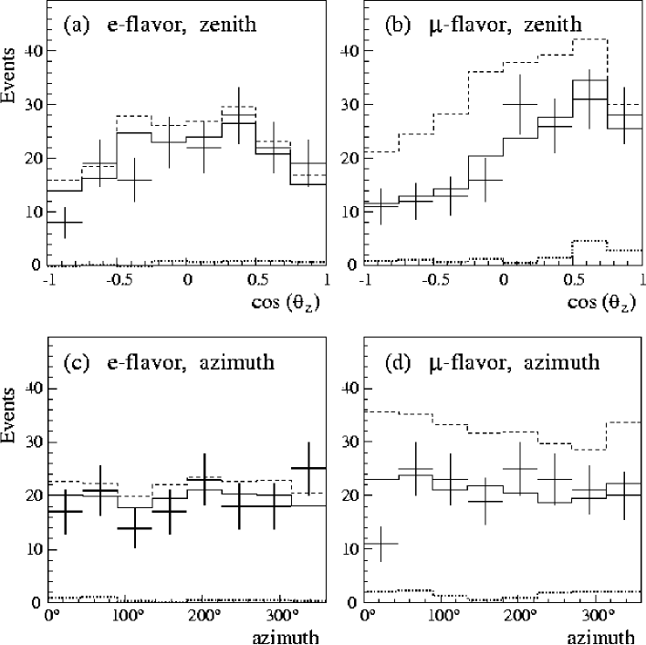
Figure 4: Angular distributions for HiRes e-flavor events (plots (a) and (c)) and $\mu$-flavor events (plots (b) and (d)). Plots (a) and (b) show the cosine of the zenith angle and plots (c) and (d) the azimuth angle. The points with error bars are the qs-data. The dashed histograms are the sum of the predicted unoscillated neutrino distribution plus the fitted qs-rock contribution. The solid histograms are the same but with the neutrino distribution weighted by the oscillation probability predicted by the best fit parameters from the analysis described in Sect. 5. The dotted histograms are the contribution of the qs-rock background. Downward going events have cos$\theta_{z}$=+1.0. Note the depletion of $\mu$-flavor events at all but the highest value of cos$\theta_{z}$.

4.2 Angular and L/E distributions

In this analysis pure two flavor $\nu_{\mu}\rightarrow\nu_{\tau}$ oscillations will be assumed, based on the absence of observed effects in the e-flavor events, shown below, and the results of the CHOOZ [23] and Super-K [1] experiments. Two flavor oscillations in vacuum leading to $\nu_{\mu}$ disappearance are described by the well-known formula:

$$P(\nu_{\mu}\rightarrow\nu_{\mu})=1.0-\sin^{2}2\theta\cdot\sin^{2}\left[1.27\mbox{ }\Delta m^{2}[\mbox{eV}^{2}]\cdot\left(\frac{L\mbox{[km] }}{E\mbox{[GeV] }}\right)\right].$$ (10)

The $\nu_{\mu}$ survival probability, $P$, is a function of $L/E$ where $L$ is the distance traveled by the neutrino and $E$ is the neutrino energy. The parameters to be determined are $\Delta m^{2}$, the mass squared difference, and $\sin^{2}2\theta$, the maximum oscillation probability.

The distance, $L$, is calculated by projecting the measured neutrino direction back to the atmosphere. It is related to the zenith angle, $\theta_{z}$, by

$$L(\theta_{z})=\sqrt{(R_{e}-d_{d})^{2}\cos^{2}\theta_{z}+(d_{d}+h)(2R_{e}-d_{d}+h)}-(R_{e}-d_{d})\cos\theta_{z}$$ (11)

where $R_{e}$ is the radius of the Earth, $d_{d}$ is the depth of the detector and $h$ is the neutrino production height in the atmosphere. The mean of the production height distribution for neutrinos of a given type, energy and zenith angle [24] was used as the estimator of $h$. The variation in production height is comparable to the path length for neutrinos coming from above the detector. The distance travelled is a function of $cos\theta_{z}$ but not of the azimuth angle. Oscillation effects are therefore expected in the shape of the zenith angle distribution but not in that of the azimuth angle distribution.

Fig. 4 shows the azimuth and zenith angle dependence of the HiRes $\mu$-flavor and e-flavor events. The effects of oscillations are most visible in the HiRes sample. The points with errors are the qs-data. The dashed histograms are the expected, unoscillated, MC neutrino contribution based on the Bartol 96 flux calculation plus the fitted qs-rock contribution. The solid histograms are the same but with the MC weighted by the oscillation probability predicted by the best fit oscillation parameters of the analysis described in Sect. 5. The dotted histograms are the fitted background qs-rock contribution. It can be seen that both the azimuth and zenith angular distributions for the e-flavor events (Figs. 4a and 4c) are consistent with the unoscillated MC prediction up to a 10-15% normalization of the overall flux. On the other hand, the $\mu$-flavor zenith angle distribution (Fig. 4b) shows a 50% deficit at large zenith angles (large $L$) but little deficit for downward going events (small $L$), confirming the observation of similar effects in the Super-K experiment. Note that at the high magnetic latitude of Soudan the azimuth angle distribution of both flavors (Figs. 4c and 4d) is predicted and observed to be flat, unlike the distribution at Kamioka where there is a pronounced East-West asymmetry.

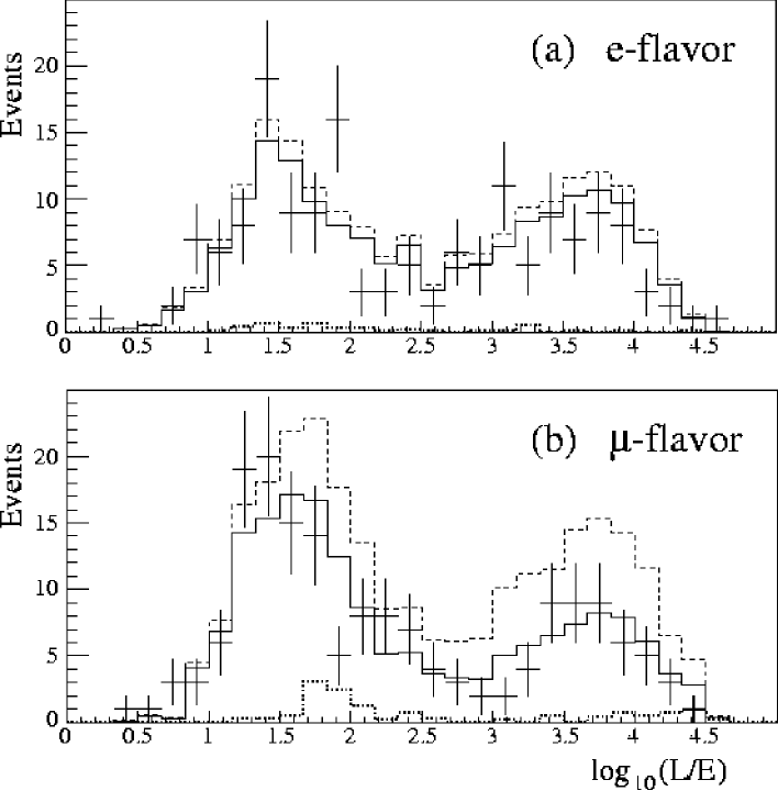
Figure 5: The HiRes $\log_{10}L/E$ distribution for e-flavor events (top) and $\mu$-flavor events (bottom). The points with errors are the qs-data. The dashed histograms are the prediction of the unoscillated Monte Carlo plus the fitted qs-rock contribution. The solid histograms are the same but with the Monte Carlo weighted by the best fit oscillation parameters from the analysis described in Sect. 5. The dotted histograms are the contribution of the qs-rock background. A depletion of $\mu$-flavor events above values of $\log_{10}L/E$ of approximately 1.5 can be seen.

Fig. 5 shows the $\log_{10}L/E$ distributions for the HiRes e-flavor and $\mu$-flavor samples. The double peaked structure is a geometrical effect, reflecting the spherical shape of the Earth. The peak at lower $\log_{10}L/E$ consists predominantly of downward-going neutrinos from the atmosphere above the detector, while the peak at higher $\log_{10}L/E$ contains upward-going neutrinos from the other side of the Earth. Again the e-flavor sample follows well the MC prediction, up to a normalization factor, indicating that within the errors of this experiment there is no evidence for $\nu_{e}$ oscillations. The $\mu$-flavor sample shows a deficit of events above a $\log_{10}L/E$ value of around 1.5. Below this value there is little, if any, loss of events. This implies an upper limit on the value of $\Delta m^{2}$ of about 0.025 eV² which is reproduced in the detailed fits described in Sect. 5.

5 Neutrino Oscillation Analysis

An extended maximum likelihood analysis assuming two-flavor $\nu_{\mu}\rightarrow\nu_{\tau}$ oscillations has been used to obtain estimates of the neutrino oscillation parameters. The significance of the result and the confidence intervals on the oscillation parameters are determined using the unified method advocated by Feldman and Cousins [9].

5.1 The likelihood function

The likelihood function used to describe the qs-data assumes that the sample is composed of neutrino interactions, represented by the Monte Carlo events, and qs-rock background events, represented by the rock sample. Each sample is divided into $\mu$-flavor, e-flavor and NC plus ambiguous events. Since neither $\nu_{e}$ or NC events are assumed to oscillate they can be considered as a single category. For shorthand in the following they are combined under the heading of e-flavor .

The $L/E$ distribution of the $\mu$-flavor events is examined for evidence of oscillations. The total number of events, $\mu$-flavor plus e-flavor, provides the normalization of the Monte Carlo exposure. Monte Carlo events with misidentified flavor are included in the $\mu$-flavor or e-flavor samples with the oscillation probabilities appropriate to their true parameters. Charged current interactions of $\nu_{\tau}$ were not generated in the Monte Carlo. At the Super-K best fit oscillation parameters, approximately two interactions producing $\tau$ leptons are expected in this data sample.

Each event in the $\mu$-flavor sample is characterized by its measured values, $(x_{i},d_{i})$, of $x\equiv$ $\log_{10}L/E$ and depth within the detector, $d$. The true value of $L/E\equiv(L/E)^{\rm true}$ is also known for each event in the Monte Carlo sample. The distinction between the five categories of $\mu$-flavor event (HiRes tracks and multiprongs, LoRes tracks and multiprongs and PCEs) is maintained for the analysis.

The log-likelihood function used is:

$${\cal{L}} = \sum_{k=1,5}\left\{\sum_{i=1,N_{\mu}^{k}}\ln Q^{k}(x_{i},d_{i})+N_{\mu}^{k}\ln M_{\mu}^{k}-M_{\mu}^{k}\right\}+N_{e}\ln M_{e}-M_{e}.$$ (12)

The function $Q^{k}(x_{i},d_{i})$ is the normalized joint $(x_{i},d_{i})$ probability density function (pdf) for category $k$ and the $k$-summation is taken over the five $\mu$-flavor event categories. The symbols $N_{\mu}^{k}$ and $N_{e}$ denote the total number of qs-data events in the $\mu$-flavor and e-flavor categories and $M_{\mu}^{k}$ and $M_{e}$ are the predicted number of events, i.e. the sum of MC neutrino plus qs-rock events. The function $Q$ represents the shape information in the $L/E$ and depth distributions and the other terms arise from the data normalization.

The joint $(x,d)$ distribution of the qs-data is the sum of the joint $(x,d)$ distributions of true neutrino events and qs-rock background events. The simplification is made that the joint distributions can be represented as the product of the distributions of $L/E$ and depth, i.e. that there is no correlation between the $L/E$ of an event and its depth in the detector. Thus the $(x,d)$ pdfs for $\mu$-flavor neutrino and qs-rock events are $X^{k}_{\mu}(x_{i})D^{k}_{\mu}(d_{i})$ and $X_{R}^{k}(x_{i})D_{R}^{k}(d_{i})$ respectively. $X^{k}_{\mu}(x_{i})D^{k}_{\mu}(d_{i})$ is the normalized probability that event $i$ of $\mu$-flavor category $k$ has a value of $\log_{10}L/E$ $=x_{i}$ and is found at a depth $d_{i}$ if it is a neutrino interaction, and $X_{R}^{k}(x_{i})D_{R}^{k}(d_{i})$ is the corresponding probability that the event arises from a rock background interaction. Substituting for $Q$ and normalizing it to 1.0, the likelihood function becomes

$${\cal{L}} = \sum_{k=1,5}\left\{\sum_{i=1,N_{\mu}^{k}}\ln\left[{{AC^{k}X^{k}_{\mu}(x_{i})D^{k}_{\mu}(d_{i})+N_{R}^{k}X_{R}^{k}(x_{i})D_{R}^{k}(d_{i})}\over{M_{\mu}^{k}}}\right]+N_{\mu}^{k}\ln M_{\mu}^{k}-M_{\mu}^{k}\right\}$$ (13)

$$+N_{e}\ln M_{e}-M_{e}\,.$$

The factor $A$ is a free parameter representing the normalization of the MC sample to the qs-data and $C^{k}$ is the oscillated number of $\mu$-flavor $\nu$ MC interactions for a given pair of oscillation parameters ($\sin^{2}2\theta,\Delta m^{2}$). $N_{R}^{k}$ is the number of qs-rock background events in $\mu$-flavor category $k$. The total expected number of $\mu$-flavor qs-data events in category $k$ is

$$M_{\mu}^{k}=AC^{k}+N_{R}^{k}.$$ (14)

where

$$C^{k} = \sum_{j=1,C^{k}_{0}}P((L/E)_{j}^{\rm true})$$ (15)

and $C^{k}_{0}$ is the total unoscillated number of MC events of category $k$. The oscillation survival probabilities, $P((L/E)^{\rm true})$ as defined in Eq. (10), are computed using the known, true, values of $L/E$ and the given oscillation parameters. The expected number of qs-data e-flavor events is given by

$$M_{e}=AC^{e}+N_{R}^{e}$$ (16)

where $C^{e}$ is the total number of Monte Carlo e-flavor events and $N_{R}^{e}$ is the number of e-flavor qs-rock events.

5.2 Probability density functions

Continuous pdfs, $X^{k}_{\mu}(x)$ and $X_{R}^{k}(x)$, are constructed from the Monte Carlo and rock samples to represent the expected neutrino and qs-rock background distributions for each category of $\mu$-flavor events. The use of a continuous pdf is preferred over the more conventional histogram representation since it does not require any arbitrary choice of binning. The pdfs are constructed by spreading the positions of the measured $x$ values of the Monte Carlo and rock events with smooth functions. This enables a continuous functional form of the pdf to be obtained from the finite set of discrete parameter values of the MC events. Explicitly the pdfs are constructed as follows:

$$X^{k}_{\mu}(x) = {1\over C^{k}}\sum_{j=1,C^{k}_{0}}g^{k}_{\mu}(x_{j}-x)P((L/E)_{j}^{\rm true})$$ (17)

where $g^{k}_{\mu}(x_{j}-x)$ is the spreading function. Likewise

$$X^{k}_{R}(x) = {1\over N^{k}_{R0}}\sum_{j=1,N^{k}_{R0}}g^{k}_{R}(x_{j}-x)$$ (18)

where $N^{k}_{R0}$ is the total number of events in the category $k$ rock sample. A normalized Gaussian form is chosen for the spreading functions,

$$g^{k}(x_{j}-x) = {1\over{{\sqrt{2\pi}\sigma_{k}}}}\exp(-(x_{j}-x)^{2}/2\sigma_{k}^{2})\,.$$ (19)

The pdfs constructed according to Equations 17–19 are normalized to unity. A different value of $\sigma_{k}$ is used for each different event category. The value of $\sigma_{k}$ is chosen to provide a representation of the pdf without statistical dips which could be mistaken for oscillation structures. The value is a balance between small values which emphasize the resolution of the experiment and larger values which smooth the finite statistics of the samples. The values of $\sigma_{k}$ used are given in Table 3.

The depth pdfs $D^{k}_{\mu}(d)$ and $D_{R}^{k}(d)$ are represented by histograms of the depth distributions similar to those shown in Fig. 3.

Event category	$\sigma$ MC	$\sigma$ rock
HiRes tracks	0.075	0.12
LoRes tracks	0.110	0.13
PCE	0.100	0.25
LoRes multiprongs	0.180	0.25
HiRes multiprongs	0.100	0.25

Table 3: Values of $\sigma$ used to construct the pdfs.

5.3 Determination of the oscillation parameters

The two oscillation parameters to be determined are $\sin^{2}2\theta,\Delta m^{2}$ for which proper coverage is provided. Seven other unknown quantities, the normalization of the MC, $A$, the five rock fractions for the different $\mu$ flavor samples and the rock fraction for the e-flavor sample are nuisance parameters. In general their fitted values will be correlated with the values of the oscillation parameters. The qs-rock background in the PCE sample is known to be very small from the small number of partially contained rock events in Table 1, the measured shield efficiency and the measured neutron energy distribution. It is set to zero in this analysis. The amount of qs-rock background in the e-flavor sample is estimated by a fit to the e-flavor depth distributions as described in Sect. 4.1.1 and is assumed to be independent of the oscillation parameters.

The negative log likelihood is calculated on a 15 $\times$ 80 grid of $\sin^{2}2\theta$ $\times$ log${}_{10}(\Delta m^{2})$ with $\sin^{2}2\theta$ between 0.0 and 1.0 and $\Delta m^{2}$ between $10^{-5}$ and $10^{0}$ eV². The $\nu_{\mu}$ survival probability, $P$, defined in Eq. (10), is averaged over the area of each grid square. The range of $\Delta m^{2}$ was chosen such that outside this range the predictions for $\log_{10}L/E$ are constant to a good approximation. Below the lower limit the survival probability is close to one for the whole $\log_{10}L/E$ range, above the upper limit the probability averages to 0.5.

At each grid square the likelihood is minimized as a function of each of the remaining four $\mu$-flavor rock fractions. The value of $A$ is calculated by requiring that the predicted number of Monte Carlo plus qs-rock events equals the number of qs-data events. For simple likelihood functions this is a mathematical condition for the minimum. It was tested and found to be a very good approximation for this likelihood function.

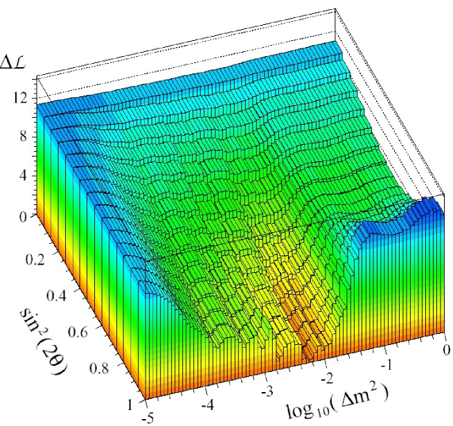
Figure 6: The data likelihood difference, $\Delta\cal{L}$, plotted as a function of $\sin^{2}2\theta$ and log${}_{10}(\Delta m^{2})$.

The lowest negative log likelihood on the grid is found and the difference between that and the value in each $\sin^{2}2\theta,\Delta m^{2}$ square ($\Delta\cal{L}$) is plotted in Fig. 6. The resulting surface exhibits a broad valley which curves from a mean value of $\sin^{2}2\theta$ of around $0.5$ at high $\Delta m^{2}$ to $\Delta m^{2}$ between $10^{-4}$ and $10^{-2}$ eV² at high $\sin^{2}2\theta$. This is the locus of constant $R_{\nu}$ as defined in Eq. (1). The shape information in the $L/E$ distribution favors the high $\sin^{2}2\theta$ region. The best likelihood occurs for the grid square centered at $\Delta m^{2}$ = 0.0052 eV², $\sin^{2}2\theta$  = 0.97. This grid square will be referred to as the best fit point. The value of $A$ is 90% of the Bartol 96 prediction and the total number of $\mu$-flavor qs-rock events is 16.8, 9.6% of the fully contained $\mu$-flavor sample. The flux normalization is discussed in more detail in Sect. 7.

Since the likelihood at each grid square is an average over the area of the square, there is no $\sin^{2}2\theta$ = 0 point in the analysis. The grid square with the lowest values of $\sin^{2}2\theta$ and $\Delta m^{2}$ is taken as a good approximation to the case of no oscillations. The likelihood rise from the minimum at this grid square is 11.3. The hypothesis of no oscillations is thus strongly disfavored. A quantitative assessment of its probability is presented in Sect. 6.2.

Fig. 6 shows that the likelihood surface is not parabolic in the region of the minimum. Errors on the parameters cannot be accurately defined using a simple likelihood rise. Confidence level contours have been determined using the method of Feldman and Cousins as described in Sect. 6.

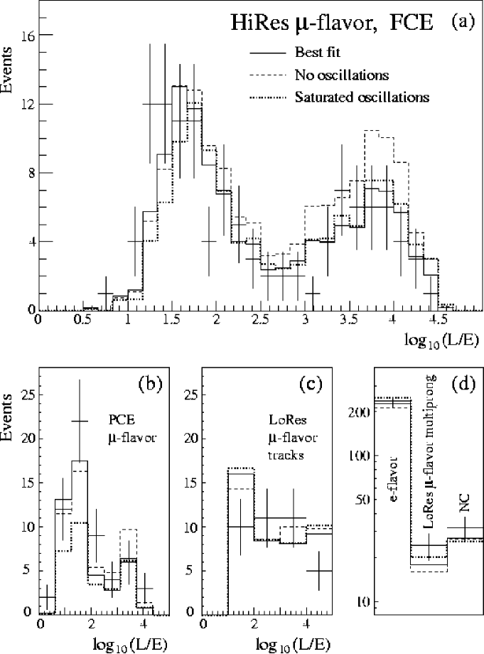
Figure 7: Comparison of the qs-data with the fit predictions. Each plot shows the qs-data as points with error bars. The sum of the neutrino Monte Carlo plus qs-rock for the best fit point in $\sin^{2}2\theta,\Delta m^{2}$ is the solid histogram. The case of no oscillations is the dashed histogram and saturated oscillations the dotted histogram. Plot (a) is the $\log_{10}L/E$ distribution for the HiRes $\mu$-flavor FCE. Plot (b) is the $\log_{10}L/E$ distribution for the $\mu$-flavor PCE. Plot (c) is the $\log_{10}L/E$ distribution for the LoRes $\mu$-flavor tracks. Plot (d) shows on a log scale the total events for the e-flavor sample (not including the NC plus ambiguous events), the LoRes $\mu$-flavor multiprongs and the NC plus ambiguous flavor events. The HiRes $\mu$-flavor FCE and PCE events which are summed in Fig. 5 are shown separately here.

5.4 Comparison with binned data

The results of an unbinned likelihood analysis are difficult to visually compare with the data. To provide such a comparison, Fig. 7 shows the qs-data plotted together with the histogram of the best fit prediction of the sum of oscillated neutrino Monte Carlo plus qs-rock background. Also histogrammed are the predictions for no oscillations (dashed histograms) and for $\sin^{2}2\theta$=1.0, $\Delta m^{2}$=1.0 eV² (dotted histograms), referred to hereafter as “saturated oscillations”. Although the oscillations in $\log_{10}L/E$ are rapid at this point, averaging to close to 0.5, the saturated oscillation histogram is not just half the no oscillation histogram because of the differences in the fitted normalization and amounts of rock background. The bin sizes in $\log_{10}L/E$ are chosen to be appropriate for the statistics, resolution and sensitivity to oscillations. Fig. 7a shows the HiRes FCE data. Note that the no oscillation hypothesis fits poorly to the high $\log_{10}L/E$ peak and saturated oscillations do not represent the low $\log_{10}L/E$ values. Fig. 7b shows the PCE data. Again the saturated oscillation hypothesis gives a bad fit to the low $\log_{10}L/E$ points. Fig. 7c shows the LoRes track events. The resolution in $\log_{10}L/E$ is poor for this sample and there is not much discrimination between oscillation hypotheses. Fig. 7d shows the summed number of events in the remaining three categories (e-flavor, LoRes $\mu$-flavor multiprongs and NC plus ambiguous events) where there is no detectable sensitivity to oscillations in their $\log_{10}L/E$ distribution. Note that the normalization of the neutrino Monte Carlo is strongly constrained by the number of e-flavor events. The variation in the predicted number of e-flavor events for the three hypotheses represents the difference in normalization of the flux required to give the best fit to these hypotheses. In the saturated oscillation case more qs-rock events are added to compensate for the neutrino events lost by oscillations.

Table 4 shows a $\chi^{2}$ comparison for the best fit, the fit with the current Super-K best fit parameters ($\Delta m^{2}$ = 0.0025, $\sin^{2}2\theta$ = 1.0) [25], the fit with no oscillations and the fit with saturated oscillations. Bins are combined to give a minimum of five events per bin for the $\chi^{2}$ calculation.

Case	HiRes FCE $\mu$	LoRes FCE $\mu$	PCE $\mu$	e-flavor	NC	Total
Best fit	14.1	10.1	3.8	0.2	0.8	29.0
No oscillations	42.9	9.7	3.9	1.4	0.9	58.9
Saturated oscillations	22.8	11.5	13.3	1.4	1.3	50.3
Super-K best fit	15.6	10.3	3.3	0.1	0.7	30.0
Number of bins	14	5	4	1	1	25

Table 4: The $\chi^{2}$ for the comparison of various $\sin^{2}2\theta,\Delta m^{2}$ predictions to binned qs-data. The four $\mu$-flavor background fractions and the normalization parameter, $A$, are variables in each case.

The $\chi^{2}$ comparison is in good agreement with what can be deduced from the likelihood surface. The best unbinned likelihood fit parameters give a good $\chi^{2}$ comparison of the binned qs-data to the prediction. The Super-K best fit parameters also give a good, though not the best, fit to the qs-data. The no and saturated oscillation hypotheses are strongly disfavored. However the systematic errors and non-Gaussian effects included in the Feldman-Cousins analysis are not included in this $\chi^{2}$ comparison. A full analysis of the no oscillation hypothesis is given in Sect. 6.2.

6 Determination of the Confidence Regions

6.1 Feldman-Cousins analysis

If all errors were Gaussian, if there were no systematic effects and if there were no physical boundaries on the parameters, a 90% confidence contour in $\sin^{2}2\theta,\Delta m^{2}$ could be obtained from the data likelihood plot shown in Fig. 6 by taking those grid squares where the likelihood rose by 2.3 above the minimum value. However this is far from the case in this analysis. The values of $\sin^{2}2\theta$ are bounded by 0.0 and 1.0 and the best fit is close to the upper bound. The errors on $L/E$ are a complicated function of the measurement errors and there are systematic errors to be taken into account.

The procedure proposed by Feldman and Cousins is a frequentist approach which uses a Monte Carlo method of allowing for these effects [9]. In their method MC experiments are generated and analyzed at each grid square on the $\sin^{2}2\theta,\Delta m^{2}$ plane. These experiments have the statistical fluctuations appropriate to the data exposure and can have systematic effects incorporated.

In this analysis each MC experiment was generated by selecting a random sample of the MC and rock events from the total sample of these events. The normalization of the MC neutrino events was based on the number of background subtracted e-flavor events and allowed to fluctuate within its statistical errors. A random amount of qs-rock background was added according to the value and error of the background estimated from the qs-data at the given $\sin^{2}2\theta,\Delta m^{2}$ grid square.

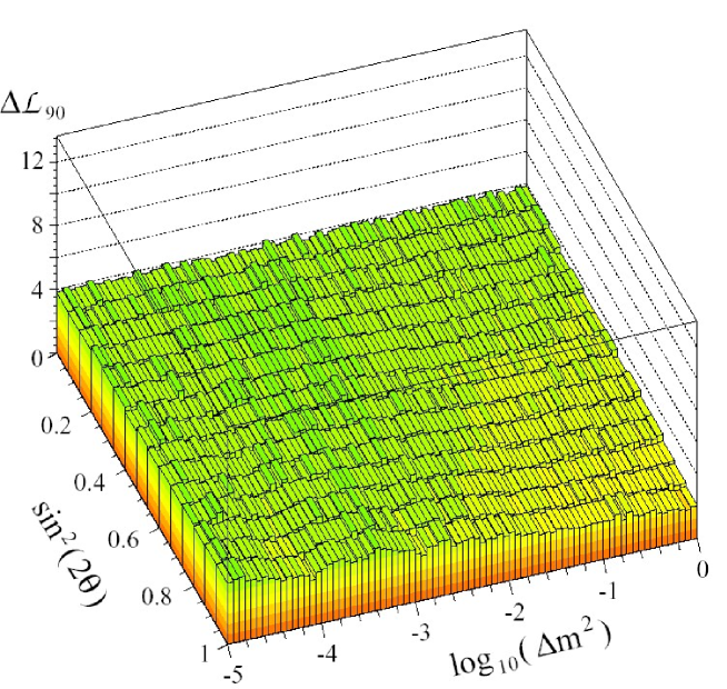
Figure 8: The 90% confidence level surface ($\Delta{\cal L}_{90}$) plotted as a function of $\sin^{2}2\theta$ and log${}_{10}(\Delta m^{2})$.

The following systematic effects were incorporated into the analysis:

1. The energy calibration of the detector has estimated errors of $\pm$7% on electron showers and $\pm$3% on muon range. In each MC experiment the calibration was varied within these errors.

2. To allow for the uncertainty in the neutrino flux as a function of energy, the predicted flux was weighted by a factor $1.0+bE_{\nu}$ where $b$ was randomly varied from 0.0 for each MC experiment with a Gaussian width of 0.005 ($E_{\nu}$ in GeV).

3. The predicted ratio of $\nu_{e}$ to $\nu_{\mu}$ events was randomly varied with a Gaussian width of 5%.

4. To allow for the uncertainties in the neutrino cross-sections, the ratio of quasi-elastic events to inelastic and deep-inelastic events was randomly varied with a Gaussian width of 20%.

In addition the method automatically included the boundary on $\sin^{2}2\theta$ and the effects of resolution and event misidentification.

Each MC experiment was analyzed in exactly the same way as the qs-data, using the same code that produced the results described in Sect. 5. The normalization of the MC flux ($A$ parameter) was determined independently for each MC experiment and the fraction of qs-rock background in each data category was fitted for each MC experiment.

One thousand MC experiments were generated at each $\sin^{2}2\theta,\Delta m^{2}$ grid square. The best fit grid square in $\sin^{2}2\theta,\Delta m^{2}$ was obtained for each experiment, not in general the same as that at which it was generated. The likelihood difference between the generated and best fit $\sin^{2}2\theta,\Delta m^{2}$ grid square ($\Delta{\cal L}_{MC}$) was calculated. A histogram of $\Delta{\cal L}_{MC}$ represents the likelihood distribution expected if the truth was at the generated grid square, including the effects of statistics and of the systematic effects. From the histogram the likelihood increase which contains 90% of the MC experiments is noted ($\Delta{\cal L}_{90}$). The plot of $\Delta{\cal L}_{90}$ as a function of $\sin^{2}2\theta,\Delta m^{2}$ is shown in Fig. 8, defining the 90% confidence surface. If the data likelihood increase at a given grid square is smaller than $\Delta{\cal L}_{90}$ in that grid square, the square is within the 90% allowed contour. Of course other likelihood contours can be obtained by taking different fractions of the MC experiments. A histogram of $\Delta{\cal L}_{MC}$ containing 100,000 experiments generated at the no oscillation grid square of $\sin^{2}2\theta,\Delta m^{2}$ is shown in Fig. 9. The peak at zero is produced by those experiments where the best fit is found at the generated grid square.

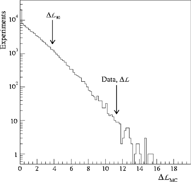
Figure 9: The Monte Carlo likelihood distribution $\Delta{\cal L}_{MC}$ for the no oscillation grid square. The values of the data likelihood ($\Delta{\cal L}$) and $\Delta{\cal L}_{90}$ are shown by the arrows.

6.2 Confidence region results

The $\Delta{\cal L}_{90}$ surface in Fig. 8 is higher than 2.3 in the no oscillation region and slopes away from this point. This is an effect of the inclusion and fitting of the qs-rock background and the constraint that the amount of qs-rock background is positive. If zero qs-rock events are generated (as frequently happened at these points since the qs-data fit prefers no background) the fit can only produce the same or more qs-rock events. More qs-rock events require a larger number of events to be lost by oscillation to match the overall normalization, therefore the best fit tends to move to larger $\sin^{2}2\theta,\Delta m^{2}$. The bias in the fits produces a broad likelihood distribution at these points and thus a high $\Delta{\cal L}_{MC}$. At the opposite corner of the plot, at large $\sin^{2}2\theta,\Delta m^{2}$, the maximum oscillation signal occurs and no larger decrease in the number of events can be obtained. Thus the fit has to remain in this same area of $\sin^{2}2\theta,\Delta m^{2}$ when statistical fluctuations decrease the number of events. The likelihood distribution is narrow and $\Delta{\cal L}_{MC}$ is decreased.

Combining Figs. 6 and 8, a 90% confidence level contour is obtained and plotted in Fig. 10, together with similar contours for the 68% and 95% confidence levels. At the 68% ($1\sigma$) level there are two regions. One corresponds to the lower part of the Super-K 90% confidence region. The other, larger region is at higher $\Delta m^{2}$ and contains the best fit point of this analysis. The data likelihood is relatively flat in the region immediately below $\Delta m^{2}$ = $10^{-3}$ eV², which is reflected in the relatively large increase in area going between 90% and 95% confidence.

The probability of the no oscillation hypothesis is given by that fraction of the MC experiments at the no oscillation grid square having $\Delta{\cal L}_{MC}>11.3$, the value of $\Delta{\cal L}$, the data likelihood rise, for this grid square. The values of $\Delta{\cal L}_{MC}$ are histogrammed in Fig. 9. Fifty-eight of the 100,000 experiments exceeded 11.3, giving a probability for the no oscillation hypothesis of $5.8\times 10^{-4}$. This probability takes account of the statistical precision of the experiment and all the systematic effects included in the Feldman-Cousins analysis.

The dotted line in Fig. 10 is the 90% confidence sensitivity, defined by Feldman and Cousins as the Monte Carlo expectation for the 90% confidence contour, given this data exposure and the best fit point of the analysis. The data 90% limit is in reasonable agreement with the expected sensitivity but lies inside the sensitivity curve, which corresponds closer to the 95% limit from the qs-data. This arises because the the flavor ratio for the qs-data is lower than that expected by the MC at the best fit point.

The thin solid line in Fig. 10 is the 90% confidence region that would be obtained by taking a simple 2.3 rise of the data likelihood, $\Delta{\cal L}$, in Fig. 6. The result of the Feldman-Cousins analysis and the inclusion of the systematic errors is to significantly increase the size of the 90% confidence region. Roughly the 68% confidence region of the full analysis corresponds to the 90% confidence region when these effects are not included.

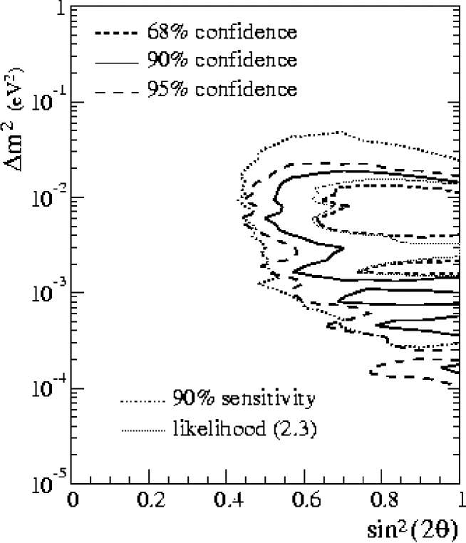
Figure 10: Confidence level contours from the Feldman-Cousins analysis, 68% (short dashed line), 90% (thick solid line) and 95% (long dashed line). The dotted line is the 90% sensitivity for the best fit $\sin^{2}2\theta,\Delta m^{2}$ point. The thin solid line is the contour defined by a data likelihood rise, $\Delta{\cal L}$, of 2.3.

A second, independent Feldman-Cousins based analysis was carried out on this data [21]. There were two main differences from the analysis described in the previous sections. Firstly, rather than fitting to continuous pdfs of $\log_{10}L/E$ distributions, binned histograms were used. Fluctuations observed depending on the bin starting point were resolved by averaging the results from many different starting points. Secondly, the backgrounds were fixed at the values determined from depth distributions as described in Sect. 4.1.1. Thus the fits were made only to the $\log_{10}L/E$ distributions using three parameters, $\sin^{2}2\theta$, $\Delta m^{2}$, and the normalization, $A$. Despite the different procedures, the results of the two analyses were in excellent agreement.

7 Flux normalization

The normalization factor $A$ and the amount of qs-rock background are subsidiary outputs from the analysis. They are calculated for each $\sin^{2}2\theta,\Delta m^{2}$ grid square. They vary slowly as a function of $\sin^{2}2\theta,\Delta m^{2}$, both being a minimum at low values of the two parameters and maximum at high values. At low values of the parameters there are no oscillation effects predicted, however the qs-data exhibits a large deficit of $\mu$-flavor events as described in Sect. 4.1. Thus to get the best fit to the qs-data the overall normalization is reduced and no qs-rock background is added. Similarly at high values of the parameters the $\mu$-flavor events are suppressed by approximately a factor of two at all $L/E$ values. In order to obtain the best compromise between the e-flavor and $\mu$-flavor events, the fit includes a larger amount of qs-rock background and requires a larger value of the normalization parameter. Within the 90% confidence allowed region of $\sin^{2}2\theta,\Delta m^{2}$, the value of $A$ lies between 85% and 92% of the prediction based on the Bartol 96 flux [18] and the NEUGEN neutrino event generator [14]. The number of background qs-rock $\mu$-flavor events lies between 5 and 30. These values are in good agreement with those obtained from the fits to the depth distributions alone, described in Sect. 4.1.1 and Table 1.

An analysis using the Battistoni 3D atmospheric neutrino flux [19] together with the neutrino production height prediction of Ref. [24] yielded very similar likelihood surfaces but with a best fit $A$ value of 105%, to be compared with 91% for the Bartol 96 flux. The major difference between the 3D and 1D fluxes, the peak at low energies towards the horizon, is washed out by the poor experimental resolution in that direction and at those energies.

8 Conclusions

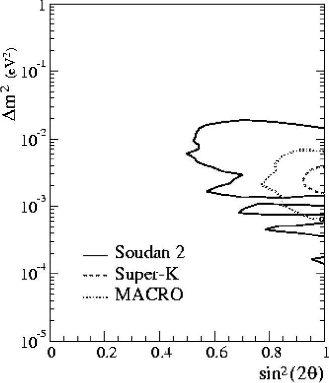
Figure 11: The Soudan 2 90% confidence allowed region in $\sin^{2}2\theta,\Delta m^{2}$ (solid line) compared with the most recent allowed regions of Super-K (dashed line) [25] and MACRO (dotted line) [26].

The Soudan 2 90% confidence allowed region is shown in Fig. 11 compared with the most recent Super-K [25] and MACRO [26] allowed regions. The result presented here is in good agreement with both experiments. From the Soudan 2 analysis the probability of the hypothesis of no oscillations is $5.8\times 10^{-4}$. There is no evidence of a departure from the predicted $L/E$ distribution of the electron events confirming that the oscillation is predominantly $\nu_{\mu}$ to $\nu_{\tau}$ or $\nu_{s}$ . The zenith angle distribution of the $\mu$ flavor events shows the same depletion as a function of angle as was observed by Super-K.

This is the first detailed study of contained and partially contained atmospheric neutrino interactions in an experiment using a detection technique, an iron calorimeter, which is very different from that of Super-K and previous water Cherenkov detectors. The event detection and reconstruction properties of Soudan 2 are different, and in many cases superior, to those of Super-K but the exposure is much smaller. The geographical locations and backgrounds of the two experiments are different. Therefore any detector systematic effect which might simulate neutrino oscillations or bias the determination of oscillation parameters is highly unlikely to be present in both experiments. The excellent agreement between the experiments is a strong confirmation of the discovery of neutrino oscillations in the atmospheric neutrino flux.

References

- [1] The Super-Kamiokande Collaboration, Y. Fukuda et al., Phys. Lett. B 433, 9 (1998); Phys. Rev. Lett. 81, 1562 (1998); Phys. Lett. B 436, 33 (1998); Phys. Rev. Lett. 85, 3999 (2000).
- [2] The SNO Collaboration, Q.R. Ahmed et al., Phys. Rev. Lett. 89, 011301 (2002); Phys. Rev. Lett. 89, 011302 (2002).
- [3] The KamLAND Collaboration, K. Eguchi et al., Phys. Rev. Lett. 90, 021802 (2003).
- [4] The K2K Collaboration, M.H. Ahn et al., Phys. Rev. Lett. 90, 041801 (2003).
- [5] The Soudan 2 Collaboration, W.W.M. Allison et al., Phys. Lett. B 391, 491 (1997); Phys. Lett. B 449, 137 (1999).
- [6] The Kamiokande Collaboration, K.S. Hirata et al., Phys. Lett. B 205, 416 (1988); Phys. Lett. B 280, 146 (1992); Y. Fukuda et al., Phys. Lett. B 335, 237 (1994).
- [7] The IMB-3 Collaboration, D. Casper et al., Phys. Rev. Lett. 66, 2561 (1991); R. Becker-Szendy et al., Phys. Rev. D 46, 3720 (1992).
- [8] The MACRO Collaboration, M. Ambrosio et al., Phys. Lett. B 517, 59 (2001).
- [9] G.J. Feldman and R.D. Cousins, Phys. Rev. D 57, 3873 (1998).
- [10] The Soudan 2 Collaboration, W.W.M. Allison et al., Nucl. Instr. Meth. A 376, 36 (1996); Nucl. Instr. Meth. A 381, 385 (1996).
- [11] The Soudan 2 Collaboration, W.P. Oliver et al., Nucl. Instr. Meth. A 276, 371 (1989).
- [12] The Soudan 2 Collaboration, see summary and references in: D. Wall et al., Phys. Rev. D 62, 092003 (2000) and C. Garcia-Garcia, Ph.D. thesis, University of Valencia, 1990.
- [13] D.A. Petyt, Soudan-2 internal note PDK-771, Sept. 2001 (unpublished).
- [14] G. Barr, D.Phil thesis, University of Oxford, 1987; H. Gallagher, Nucl. Phys. B (Proc. Suppl.) 112, 188 (2002).
- [15] H. Fesefeldt, “GHEISHA, the simulation of hadronic showers: physics and applications”, Aachen Tech. Hochsch., Aachen, Germany, 1985.
- [16] W.R. Nelson, H. Hirayama and D.W. Rogers, “The EGS4 Code System”, SLAC, Stanford, CA, December 1985; R.L. Ford and W.R. Nelson, “EGS 3 Electron Gamma Shower”, SLAC Report 210 (1978).
- [17] G. Barr, T.K. Gaisser and T. Stanev, Phys. Rev. D 39, 3532 (1989).
- [18] V. Agrawal, T.K. Gaisser, P. Lipari and T. Stanev, Phys. Rev. D 53, 1313 (1996).
- [19] G. Battistoni et al., Astropart. Phys. 12, 315 (2000); G. Battistoni, A. Ferrari, T. Montaruli, and P.R. Sala, astro-ph/0207035, July 2002. Flux tables for the Soudan site are available at http://www.mi.infn.it/battist/neutrino.html.
- [20] University of New Hampshire, Neutron Monitor Datasets, National Science Foundation Grant ATM-9912341, http://ulysses.sr.unh.edu/NeutronMonitor/neutron_mon.html.
- [21] M. Sanchez, Ph.D. thesis, Tufts University (2003).
- [22] R. Barlow and C. Beeston, Comp. Phys. Comm. 77, 219 (1993); R. Barlow, J. Comp. Phys. 72, 202 (1987). The method was implemented both in the CERN program MINUIT, CERN Program Library Long Writeup Y250, and in an independent program developed by this collaboration.
- [23] The CHOOZ Collaboration, M. Apollonio et al., Phys. Lett. B 466, 415 (1999).
- [24] H. Gallagher and K. Ruddick, Soudan-2 internal note PDK-784, Jan. 2002 (unpublished).
- [25] C. Yanagisawa, for the Super-Kamiokande Collaboration. Presented at NOON ’03, Kanazawa, Japan, www-sk.icrr.u-tokyo.ac.jp/noon2003, February 2003.
- [26] The MACRO Collaboration, M. Ambrosio et al., hep-ex/0304037, April 2003.