Light quark and charm interplay in the Dalitz-plot analysis of hadronic decays in FOCUS

Abstract

The potentiality of interpreting the $D$-meson decay-dynamics has revealed itself to be strongly dependent on our understanding of the light-meson sector. The statistics collected by FOCUS is already at a level that manifests parametrization problems for scalar particles. In this paper the first application of the $K$-matrix approach in the charm sector is illustrated and preliminary results on the $D^{+}$ and $D_{s}$ decays to three pions are shown.

1 Introduction

Charm-meson decay-dynamics has been studied extensively over the last decade. Dalitz plot analysis has indeed revealed itself a powerful tool for investigating the effects of resonant substructures, interference patterns and final-state interactions in the charm sector. The isobar formalism traditionally applied consists of a sum of relativistic Breit–Wigner resonances properly modulated by form factors (Blatt–Weisskopf barrier factors are generally used) and multiplied by an angular term assuring angular-momentum conservation. The potentiality to investigate charm dynamics has revealed itself to be strongly connected with a knowledge of the light-meson sector. In particular, the need to model the scalar particles populating our charm-meson Dalitz plots has led us to question the validity of the BW approximation for the description of a resonance. Resonances are associated with poles of the $S$-matrix in the complex energy plane. It is the position of the pole that provides the fundamental, model-independent, process-independent resonance parameters.

The fitting of data with simple Breit–Wigner formulæ corresponds to the most elementary type of extrapolation from the physical region to an unphysical-sheet pole. In the case of a narrow, isolated resonance, there is a close connection between the position of the pole on the unphysical sheet and the peak we observe in experiments at real values of the energy. However, when a resonance is broad and overlaps with other resonances, this connection is lost. The BW parameters measured on the real axis (mass and width) can be connected to the pole-positions in the complex energy plane only through models of analytic continuation. A formalism for studying overlapping and many channel resonances was proposed long ago and is based on the $K$-matrixwigner ; chung parametrization. This formalism, originating in the context of two-body scattering, can be generalized to cover the case of resonance production in more complex reactions, with the assumptions that the two-body system in the final state is isolated and that the two particles do not simultaneously interact with the rest of the final state in the production processaitch . Its implementation allows us to include the positions of the poles in the complex plane directly in our analysis, embedding in our amplitudes the results from spectroscopy experimentspenn1 ; anisar1 .

2 The fit formalism

The formalism traditionally applied to three-body charm decays relies on the so-called isobar model. A resonant amplitude for a quasi-two-body channel, of the type

$$\begin{array}[]{cl}D\to&r+c\\[-2.15277pt] &\kern 1.49994pt\raise 5.16663pt\hbox{$|$}\kern-4.79996pt\to a+b\,,\end{array}$$

is interpreted à la Feynman. For the decay $D\to\pi\pi\pi$ of Fig. 1,

Figure 1: The $D^{+}\to\pi\pi\pi$ decay diagram.

a $D\to\pi$ current with form factor $F_{D}$ interacts with a di-pion current with form factor $F_{r}$ through an unstable propagator with an imaginary width contribution in the propagator mass. Each resonant decay function is thus,

$$A=F_{D}F_{r}\times|\bar{c}|^{J}|\bar{a}|^{J}P_{J}(\cos\Theta^{r}_{ac})\times BW(m_{ab})\,$$ (1)

i.e., the product of two vertex form factors (Blatt–Weisskopf momentum-dependent factors), a Legendre polynomial of order $J$ representing the angular decay wave function, and a relativistic Breit–Wigner (BW). In this approach, already applied in the previous analyses of the same channels e687_dpds ; e791_dpds , the total amplitude (Eq. 2) is assumed to consist of a constant term describing the direct non-resonant three-body decay and a sum of functions (Eq. 1) representing intermediate two-body resonances.

$$A(D)=a_{0}e^{i\delta_{0}}+\sum_{i}a_{i}e^{i\delta_{i}}A_{i}\,,$$ (2)

Additional care has to be applied to describe the $f_{0}(980)$ resonance because of the opening of the $K\mathchoice{\makebox[0.0pt][l]{$\displaystyle\kern 2.05pt\overline{\kern-2.3917pt\phantom{K}\kern-0.43057pt}$}}{\makebox[0.0pt][l]{$\textstyle\kern 2.05pt\overline{\kern-2.3917pt\phantom{K}\kern-0.43057pt}$}}{\makebox[0.0pt][l]{$\scriptstyle\kern 1.435pt\overline{\kern-1.67418pt\phantom{K}\kern-0.3014pt}$}}{\makebox[0.0pt][l]{$\scriptscriptstyle\kern 1.025pt\overline{\kern-1.19585pt\phantom{K}\kern-0.21529pt}$}}K$ channel near its pole mass. A Flatté coupled-channel parametrization e687_dpds ; flatte is generally adopted.

2.1 The $K$-matrix formalism

For a well-defined wave of specific isospin and spin IJ, characterized by narrow and isolated resonances the propagator is, as anticipated, of the simple BW form. In contrast, when the specific wave IJ is characterized by large and heavily overlapping resonances, just as the scalars, the propagation is no longer dominated by a single resonance, but is the result of complicated interplay among the various resonances. In this case, it can be demonstrated on very general grounds that the propagator may be written in the context of the $K$-matrix approach as

$$(I-iK\cdot\rho)^{-1}$$ (3)

where K is the matrix for the scattering of particle $a$ and $b$ and $\rho$ is the phase-space matrix.

While the need for a $K$-matrix parametrization, or in general for a more accurate description than the isobar model, is questionable for the vector and tensor amplitudes, since the resonances are relatively narrow and well isolated, this parametrization is unavoidable for the correct treatment of the scalar amplitudes. Indeed the $\pi\pi$ scalar resonances are large and overlap each other in such a way that it is impossible to single out the effect of any one of them on the real axis.

In order to write down the propagator, we need the scattering matrix. To perform a meaningful fit to our three-pion data, we thus need a full description of the scalar resonances in the relevant energy range, updated to the most recent measurements in this sector. To our knowledge, the only self-consistent description of $s$-wave isoscalar scattering is that given in the $K$-matrix representation by Anisovich and Sarantsev in anisar1 through a global fit of all the available scattering data from the $\pi\pi$ threshold up to 1900 MeV.

To introduce the $K$-matrix formalism used in this analysis, we must recall some general, non-trivial, considerations. The production of an isoscalar, $s$-wave state with an accompanying pion, involves, in the energy region relevant to this analysis, five channels, namely $1=\pi\pi$, $2=K\mathchoice{\makebox[0.0pt][l]{$\displaystyle\kern 2.05pt\overline{\kern-2.3917pt\phantom{K}\kern-0.43057pt}$}}{\makebox[0.0pt][l]{$\textstyle\kern 2.05pt\overline{\kern-2.3917pt\phantom{K}\kern-0.43057pt}$}}{\makebox[0.0pt][l]{$\scriptstyle\kern 1.435pt\overline{\kern-1.67418pt\phantom{K}\kern-0.3014pt}$}}{\makebox[0.0pt][l]{$\scriptscriptstyle\kern 1.025pt\overline{\kern-1.19585pt\phantom{K}\kern-0.21529pt}$}}K$, $3=\eta\eta$, $4=\eta\eta^{\prime}$ and $5=\;$multi-meson states (mainly four-pion states at $\sqrt{s}<1.6$ GeV). The production amplitude in the particular channel $(00^{++})_{i}\pi$ can be written as

$$F_{i}=(I-iK\rho)_{ij}^{-1}P_{j}$$ (4)

where $I$ is the identity matrix, $K$ is the $K$-matrix describing the isoscalar $s$-wave scattering process, $\rho$ is the phase-space matrix for the five channels, and $P$ is the ‘initial’ production vector into the five channels. In this picture, the production process is viewed as consisting of an initial preparation of several states, which then propagate via the term $(I-iK\rho)^{-1}$ into the final state. In particular, the three-pion final state can be fed by an initial formation of $(\pi\pi)\pi$, $(K\mathchoice{\makebox[0.0pt][l]{$\displaystyle\kern 2.05pt\overline{\kern-2.3917pt\phantom{K}\kern-0.43057pt}$}}{\makebox[0.0pt][l]{$\textstyle\kern 2.05pt\overline{\kern-2.3917pt\phantom{K}\kern-0.43057pt}$}}{\makebox[0.0pt][l]{$\scriptstyle\kern 1.435pt\overline{\kern-1.67418pt\phantom{K}\kern-0.3014pt}$}}{\makebox[0.0pt][l]{$\scriptscriptstyle\kern 1.025pt\overline{\kern-1.19585pt\phantom{K}\kern-0.21529pt}$}}K)\pi$, etc. The particular process we are dealing with, $(\pi^{+}\pi^{-})\pi^{+}$, is then described by the amplitude $F_{1}$.

In this paper, the $K$-matrix used is that of anisar1 :

$$K_{ij}^{00}(s)=\left\{\sum_{\alpha}\frac{g^{(\alpha)}_{i}g^{(\alpha)}_{j}}{m^{2}_{\alpha}-s}+f^{\mathrm{scatt}}_{ij}\frac{1\,\mathrm{GeV}^{2}-s_{0}^{\mathrm{scatt}}}{s-s_{0}^{\mathrm{scatt}}}\right\}\times\frac{s-s_{A}/2m^{2}_{\pi}}{(s-s_{A0})(1-s_{A0})}.$$ (5)

The factor $g^{(\alpha)}_{i}$ is the coupling constant of the $K$-matrix  pole $\alpha$ to meson channel $i$; the parameters $f^{\mathrm{scatt}}_{ij}$ and $s_{0}^{\mathrm{scatt}}$ describe a smooth part of the $K$-matrix elements; the factor $\frac{s-s_{A}/2m^{2}_{\pi}}{(s-s_{A0})(1-s_{A0})}$ suppresses a false kinematical singularity in the physical region near the $\pi\pi$ threshold (Adler zero). The parameter values used in this analysis are listed in Table 1.

K-matrix mass poles	$g_{\pi\pi}$	$g_{K\mathchoice{\makebox[0.0pt][l]{$\displaystyle\kern 1.435pt\overline{\kern-1.67418pt\phantom{K}\kern-0.3014pt}$}}{\makebox[0.0pt][l]{$\textstyle\kern 1.435pt\overline{\kern-1.67418pt\phantom{K}\kern-0.3014pt}$}}{\makebox[0.0pt][l]{$\scriptstyle\kern 1.0045pt\overline{\kern-1.17192pt\phantom{K}\kern-0.21098pt}$}}{\makebox[0.0pt][l]{$\scriptscriptstyle\kern 0.7175pt\overline{\kern-0.83708pt\phantom{K}\kern-0.1507pt}$}}K}$	$g_{4\pi}$	$g_{\eta\eta}$	$g_{\eta\eta^{\prime}}$
0.65100	0.24844	-0.52523	0.00000	-0.38878	-0.36397
1.20720	0.91779	0.55427	0.00000	0.38705	0.29448
1.56122	0.37024	0.23591	0.62605	0.18409	0.18923
1.21257	0.34501	0.39642	0.97644	0.19746	0.00357
1.81746	0.15770	-0.17915	-0.90100	-0.00931	0.20689
$s_{0}^{\mathrm{scatt}}$	$f^{\mathrm{scatt}}_{11}$	$f^{\mathrm{scatt}}_{12}$	$f^{\mathrm{scatt}}_{13}$	$f^{\mathrm{scatt}}_{14}$	$f^{\mathrm{scatt}}_{15}$
-3.30564	0.26681	0.16583	-0.19840	0.32808	0.31193
$s_{A}$	$s_{A0}$
1.0	-0.2

Table 1: $K$-matrix parameters.

These K-matrix values correspond to a $T$-matrix description of five poles whose masses and half-widths, in GeV, are (1.019, 0.038), (1.306, 0.167), (1.470, 0.960), (1.489, 0.058) and (1.749, 0.165); the analysis in anisar1 does not require the $\sigma$. The decay amplitude for the $D$ meson into three-pion final state, where $\pi^{+}\pi^{-}$ are in a $(IJ^{PC}=00^{++}$)-wave, is thus written as

$$A(D\to(\pi^{+}\pi^{-})_{00^{++}}\pi^{+})=F_{1}=(I-iK\rho)^{-1}_{1j}\qquad$$

$$\times\left\{\sum_{\alpha}\frac{\beta_{\alpha}g_{j}^{(\alpha)}}{m^{2}_{\alpha}-m^{2}}+f_{1j}^{\mathrm{prod}}\frac{1\,\mathrm{GeV}^{2}-s_{0}^{\mathrm{prod}}}{s-s_{0}^{\mathrm{prod}}}\right\}\times\frac{s-s_{A}/2m^{2}_{\pi}}{(s-s_{A0})(1-s_{A0})}.$$ (6)

where $\beta_{\alpha}$ is the coupling to the pole $\alpha$ in the ‘initial’ production process, $f_{1j}^{\mathrm{prod}}$ and $s_{0}^{\mathrm{prod}}$ are the $P$-vector background parameters. In the end, the complete decay amplitude of the $D$ meson into three-pion final state is:

$$A(D)=a_{0}e^{i\delta_{0}}+\sum_{i}a_{i}e^{i\delta_{i}}A_{i}+F_{1}$$ (7)

where the index $i$ now runs only over the vector and tensor resonances, which can be safely treated as simple Breit–Wigner’s (see Eq. 1). In the fit to our data, the $K$-matrix parameters are fixed to the values of Table 1, which consistently reproduce measured s-wave isoscalar scattering. The free parameters are those peculiar to the $P$-vector, i.e. $\beta_{\alpha}$, $f^{\mathrm{prod}}_{1j}$ and $s_{0}^{\mathrm{prod}}$, and those in the remaining isobar part of the amplitude, $a_{i}$ and $\delta_{i}$.

3 Three-pion preliminary results

The three-pion selected samples (Fig. 2) consist of $1527\pm 51$ and $1475\pm 50$ events for the $D^{+}$ and $D_{s}$ respectively. The Dalitz plot analyses are performed on yields within $\pm 2\sigma$ of the fitted mass value.

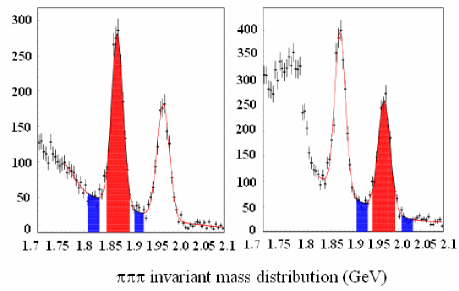
Figure 2: $D^{+}$ and $D_{s}$ signals and sideband regions.

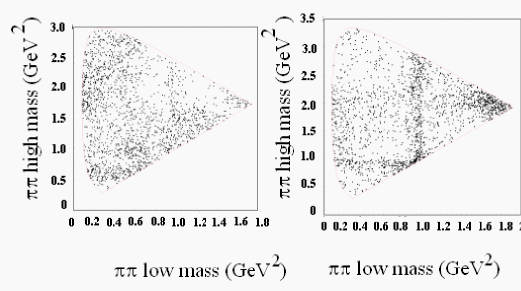
Figure 3: Three-pion $D^{+}$ and $D_{s}$ Dalitz plots.

3.1 $D_{s}\to\pi\pi\pi$

The $D_{s}$ Dalitz plot (Fig. 3) is clearly structured. Indeed, two $f_{0}(980)$ bands in the low and high projection at 1000 MeV, a band in the 1500 MeV high-projection region and an accumulation of events in the corner of the folded plot are easily recognized.

resonance	fit fraction(%)	phase (deg)
NR	25.5 $\pm$ 4.6	246.5 $\pm$ 4.7
$f_{2}(1275)$	9.8 $\pm$ 1.3	140.2 $\pm$ 9.2
$f_{0}(980)$	94.4 $\pm$ 3.8	0(fixed)
$S_{0}(1475$	17.4 $\pm$ 3.1	249.7 $\pm$ 6.4
$\rho^{0}(1450)$	4.1 $\pm$ 1.0	187.3 $\pm$ 15.3

Table 2: $D_{s}$ fit fractions and phases with the isobar model.

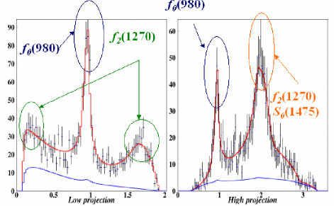
Figure 4: $D_{s}$ Dalitz plot projections and isobar fit results

When the isobar model is applied, satisfactory fits can be obtained letting only the $f_{0}(980)$ and $f_{0}(1500)$ parameters float freely. We obtain $m_{0}=975\pm 10$ MeV, $\Gamma_{\pi\pi}=90\pm 30$ MeV and $\Gamma_{KK}=35\pm 15$ MeV for the $f_{0}(980)$ and $m_{0}=1475\pm 10$ MeV and $\Gamma_{0}=112\pm 24$ MeV for the $f_{0}(1500)$. The fit C.L., evaluated with a $\chi^{2}$ estimator over a Dalitz plot with bin size adaptively chosen according to the statistics is 11.5%. The fit results are reported in Table 2.

resonance	fit fraction(%)	phase (deg)
$s-wave$	87.8 $\pm$ 1.7	0(fixed)
$f_{2}(1275)$	11.5 $\pm$ 1.2	120.3 $\pm$ 5.4
$\rho^{0}(1450)$	5.4 $\pm$ 1.1	198.6 $\pm$ 9.3

Table 3: $D_{s}$ fit fractions and phases with the $K$-matrix model.

All the established resonances decaying to $\pi^{+}\pi^{-}$ with a sizeable branching ratio are first considered in the fit. The set of contributions reported in Table 2 refers to fit coefficients of more than $2\sigma$ statistical significance. A fit with the $f_{0}(1500)$ parameters fixed to the PDG values has been also performed; the C.L. is 1% and the non-resonant fit fraction increases to about 40% (to be compared with the value in Table 2), indicating how the flat non-resonant component, not having particular signatures, absorbs the residual parametrization problems. A large systematic effect should thus be associated with this channel decay fraction weakening the potentiality to establish a reliable estimate of the annihilation processes. The projection fit results are shown in Fig. 4. It is interesting to note that the sum of the fit fractions is about 150%, pointing to a large, rather suspicious, interference effect among the contributions.

One of the main advantages of the $K$-matrix approach is the straight-forward prescription for constraining the amplitudes to respect the two-body unitarity and the universality of the poles in the complex energy plane. The resonance parameters are fixed to the reference paper anisar1 . The results are quoted in Table 3. The contribution of the whole $s$-wave in the $D_{s}$ decay into three pions is computed in a single fit fraction. The fit C.L. is 3.2%. It is interesting to note here that the sum of the fit fractions is very close to 100%. The fractions of $f_{2}(1275)$ and $\rho^{0}(1450)$ are quite consistent in the two approaches; the main difference concerns the scalar sector. A good fit to our $D_{s}\to 3\pi$ signal can be obtained even without the non-resonant contribution. The $K$-matrix fit results are shown on the Dalitz projections in Fig. 5.

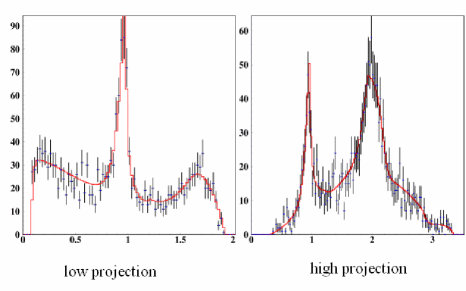
Figure 5: $D_{s}$ Dalitz-plot projections with $K$-matrix fit results.

3.2 $D^{+}\to\pi\pi\pi$

The $D^{+}\to\pi^{+}\pi^{-}\pi^{+}$ channel shows an excess of events at low $\pi\pi$ mass, (Fig. 6), which cannot be explained with simple BW’s corresponding to well-established resonances. A fit performed with a free parameter single-channel Breit–Wigner returns a mass $m=443\pm 27$ and width $\Gamma=443\pm 80$. The decay fraction and phases are reported in Table 4. The $f_{0}(980)$ parameters are fixed to the values found in the $D_{s}$ channel, where its signal is statistically more robust. The fit C.L. is about 10%; when the low-energy BW, $\sigma$, is removed the C.L. drops to $10^{-8}$.

resonance	fit fraction(%)	phase (deg)
NR	9.8 $\pm$ 4.3	0(fixed)
$f_{2}(1275)$	12.3 $\pm$ 2.1	-213.3 $\pm$ 17.7
$f_{0}(980)$	6.7 $\pm$ 1.5	-145.9 $\pm$ 17.7
$\rho(770)$	32.8 $\pm$ 3.8	62.9 $\pm$ 16.8
$S_{0}(1475)$	1.8 $\pm$ 1.2	242.3 $\pm$ 25.8
$f_{0}(400)$	18.9 $\pm$ 5.3	- 96.9 $\pm$ 30.7

Table 4: $D^{+}$ fit fractions and phases with the isobar model.

When the $K$-matrix approach is applied to the $D^{+}$, it is found that the $P$-vector degrees of freedom are able to reproduce the features of the low-energy $\pi\pi$ distribution with a fit C.L. of about 3.5%. The $K$-matrix fit results on the $D^{+}$ Dalitz projections are shown in Fig. 7; the fit fractions and phases are reported in Table 5.

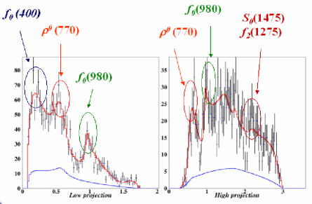
Figure 6: $D^{+}$ Dalitz-plot projections and the isobar model fit results.

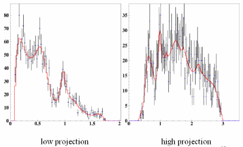
Figure 7: $D^{+}$ Dalitz-plot projections with the $K$-matrix formalism.

resonance	fit fraction(%)	phase (deg)
$s-wave$	66.5 $\pm$ 4.2	101.8 $\pm$ 22.5
$f_{2}(1270)$	11.4 $\pm$ 1.4	247.0 $\pm$ 9.0
$\rho^{0}(770)$	21.2 $\pm$ 4.4	0(fixed)

Table 5: $D^{+}$ fit fractions and phases with the $K$-matrix model.

4 Conclusions

The $K$-matrix approach has been applied for the first time to the three-pion Dalitz-plot analysis in FOCUS. The results are extremely encouraging since the same parametrization of two-body resonances coming from light-quark experiments also works for charm decays; this result was not obvious beforehand. In the $D^{+}\to\pi\pi\pi$ channel a good C.L. fit is obtained even without the $\sigma$, suggesting that a lot of work has still to be done before solving the $\sigma$ puzzle. A global fit including the charm data and the analysis of the $KK\pi$ channel could add important experimental information. The method explained here will find its full application to forthcoming excellent statistics of the charm experiments.

References

- (1) E.P. Wigner, Phys. Rev 70 (1946) 15.
- (2) S.U. Chung et al., Ann. Physik 4 (1995) 404.
- (3) I.J.R. Aitchison, Nucl. Phys. A187 (1972) 417.
- (4) K.L. Au, D. Morgan, M.R. Pennington, Phys. Rev. D35 (1987) 1633; M.R. Pennington hep-ph/9905241.
- (5) V.V. Anisovich, A.V. Sarantsev, Eur. Phys. J. A16 (2003) 229.
- (6) P.L. Frabetti et al., Phys. Lett. B407 (1997) 79.
- (7) E.M. Aitala et al., Phys. Rev. Lett. 86 (2001) 765; Phys. Rev. Lett. 86 (2001) 770.
- (8) S.M. Flatté, Phys. Lett. B63 (1976) 228.