Searching for $\eta\to\gamma\gamma\gamma$ decay

Abstract

Data collected by the KLOE experiment in years 2001/2002 for a total integrated luminosity of 410 pb^-1, corresponding to 17 million of produced $\eta$’s from the $\Phi\to\eta\gamma$ radiative decay, have been analyzed to look for the C-violating decay $\eta\to\gamma\gamma\gamma$. The signal is searched in events with 4 photons in the final state by using the spectrum of the most energetic photon. The background is evaluated from the data themself, doing a fifth degree polynomial fit outside the signal region, and extrapolating inside it. No signal has been observed and taking into account a selection efficiency $\epsilon=20.3\%$ we get from a likelihood fit Br$(\eta\to\gamma\gamma\gamma)\leq 1.6\times 10^{-5}$ at 95% CL. The procedure has a systematic ambiguity at the 35 $\%$ level.

, , , , , , , , , , , , , , , , , , , , , , , , , , , , , , , , , , , , , , , , , , , , , , , , , , , , , , , , , , , , , , , , , , , , , , , , , , , , , , , , , , , , , , , , , , , , , , , , , , , ,

1 Introduction

At the Frascati $\phi$ factory DA$\Phi$NE [1] a large number of $\eta$ mesons is produced via the radiative decay of the $\phi$ meson.

The $\phi$ mesons are produced in the collision of $e^{+}e^{-}$ beams into the DA$\Phi$NE collider and 1.298 % of them decay into the $\eta\gamma$ final state. Up to now $17\times 10^{6}$ $\eta$ mesons have been produced and are present in 410 pb^-1 collected by the KLOE experiment in years 2001-2002.

The $\eta$ meson is an even eigenstate of the charge coniugation operator C, while a photon is an odd C eigenstate. So any decay of the $\eta$ meson into a final state with an odd number of photons violates the C symmetry. In the Standard Model, the C symmetry is exactly conserved in both strong and electromagnetic decays, but it is violated in weak decays due to the V-A structure of the weak couplings. In the framework of the Standard Model the decay rate of the $\pi^{0}\rightarrow 3\gamma$ has been evaluated [2], and generalizing this result to the $\eta$ case [3], one obtains Br$(\eta\rightarrow 3\gamma)<10^{-12}$.
For this reason the discovery of a larger decay rate would be a clear signal of SM violation. At the moment all the predictions of alternative models are far below the experimentally achievable limits [3].

From the experimental point of view the only published result is that of GAMS2000 experiment (1984) which has obtained the upper limit $5\times 10^{-4}$ at 90 % C.L. [4]. There is also a preliminary result from Crystall Ball collaboration (AGS/CB) at Brookhaven which sets the limit at $1.8\times 10^{-5}$ at 90 % C.L [3]. Both the above experiments are of fixed target type, in which the $\eta$ meson is produced through the reaction $\pi^{-}p\rightarrow\eta n$ with $P_{\pi^{-}}=30$ GeV/c for GAMS and 760 MeV/c for AGS/CB.

2 Kloe detector

The detector consists of a large cylindrical drift chamber, DC [5], surrounded by a lead-scintillating fiber sampling calorimeter, EMC [6], both immersed in a solenoidal magnetic field of 0.52 T with the axis parallel to the beams. The DC tracking volume extends from 28.5 to 190.5 cm in radius and is 340 cm in length. For charged particles the transverse momentum resolution is $\delta p_{T}/p_{T}\simeq 0.4\%$ and vertices are reconstructed with a spatial resolution of $\sim$ 3 mm. The calorimeter is divided into a barrel and two endcaps and covers 98$\%$ of the solid angle. Photon energies and arrival times are measured with resolutions $\sigma_{E}/E=0.057/{\small\sqrt{E\ ({\rm GeV})}}$ and $\sigma_{t}=54\ {\rm ps}/{\small\sqrt{E\ ({\rm GeV})}}\oplus 50\ {\rm ps}$ respectively. The photon entry points are determined with an accuracy $\sigma_{l}\sim 1\ {\rm cm}/{\small\sqrt{E\ ({\rm GeV})}}$ along the fibers, and $\sim 1$ cm in the transverse directions. A photon is defined as a calorimeter cluster not associated to a charged particle, by requiring that the distance along the fibers between the cluster centroid and the impact point of the nearest extrapolated track be greater than 3$\sigma_{l}$. Two small calorimeters, QCAL [7], made with lead and scintillating tiles are wrapped around the low-beta quadrupoles to complete the hermeticity.

The trigger [8] uses information from both the calorimeter and the drift chamber. The EMC trigger requires two local energy deposits above threshold ($E>50$ MeV in the barrel, $E>150$ MeV in the endcaps). Recognition and rejection of cosmic-ray events is also performed at the trigger level, checking for the presence of two energy deposits above 30 MeV in the outermost calorimeter planes. The DC trigger is based on the multiplicity and topology of the hits in the drift cells. The trigger has a large time spread with respect to the beam crossing time. It is however synchronized with the machine radio frequency divided by four, $T_{\rm sync}$ = 10.85 ns, with an accuracy of 50 ps. During the period of data taking the bunch crossing period at DA$\Phi$NE was $T$ = 5.43 ns. The $T_{0}$ of the bunch crossing producing an event is determined offline during the event reconstruction.

3 Background

The signal in this analysis is $\phi\to\gamma\eta(\to 3\gamma)\to 4\gamma$, the cross section corresponding to the PDG2002 upper limit is very low: $<$ 0.0215 nb (at KLOE the $\phi$ production cross section is about 3 $\mu$b). So, background studies should cover all possible neutral processes at KLOE. The most important process which gives 4 photons in the final state is $e^{+}e^{-}\to\omega\gamma$ with $\omega\to\pi^{0}\gamma$ but also important are processes with less or more than 4 photons in final state which mimic 4 photons events because of cluster splitting or merging and accidental clusters due to machine background. The agreement with MC in the background description is very hard to obtain due to the above effects which are very difficult to reproduce; so we have estimated the background directly from data and used the MC only to evaluate the detection efficiency of the signal.

To this aim a generator of $\eta\to$$\gamma\gamma\gamma$ with pure phase space for the decay dynamics has been used to produce 120,000 $\phi\to\gamma\eta(\eta\to 3\gamma)$ events.

4 Event selection

First a preselection is applied to the reconstructed events of the neutral radiative stream. A ’recover splitting’ procedure (applied both to data and to MC events) is implemented to reduce the number of split clusters; moreover it is required that every cluster does not have an association with a DC track. Reconstructed data also include beam position [8] and $\phi$ energy momentum determination, obtained run by run from the analysis of Bhabha events. MC includes cluster time offset correction, and simulation of software filters used to select events for the neutral radiative stream.

The following cuts are applied to the events:

1) Ntime=4

Requires 4 photons with the correct time of flight $t$ : $|t-r/c|<5\sigma_{t}$ ; $r$ being the distance of the cluster from I.P. and $\sigma_{t}$ being the calorimeter time resolution.

2) Ngood = 4

A good photon is defined in the following way: cluster energy $>30$MeV, $|cos\theta|<0.93$, where $\theta$ is the angle respect to the beam direction. Cluster energy cut helps to reject accidental clusters and split clusters, while the polar angle cut excludes the blind region around the beam-pipe.

3) Total energy of prompt clusters $>$ 800 MeV

4) Total momentum $<$ 200MeV

These last two cuts reject events from channels with more than 4 photons in the final state which give background if some photons are lost.

The events that pass the above preselection criteria are stored in reduced files and to them are applied the following additional cuts:

5) $\theta_{\gamma\gamma}$$>$15^∘

$\theta_{\gamma\gamma}$ is the minimum angle between two photons, to further reject split clusters, which mainly come from 3$\gamma$ final states.

6) $E_{min}>50$ MeV, $|cos\theta|$ $<$ 0.91.

These cuts further reject accidental clusters and QED background.

5 Kinematic fit

At this point a kinematic fit procedure is applied to the four photons to improve the energy resolution. The input variables of the fit are the following:

• X,Y,Z coordinates of the cluster;

• E energy of the cluster;

• t time of the cluster;

• X,Y,Z of the interaction vertex;

• E,Px,Py,Pz of the $\phi$ meson.

The fit is made according to the Lagrange’s multipliers method, minimizing the following $\chi^{2}$:

$$\chi^{2}=\sum_{i}{\frac{(x_{i}-\mu_{i})^{2}}{\sigma_{i}^{2}}}+\sum_{j}{\lambda_{j}F_{j}(\mu_{k})}$$ (1)

with 27 free parameters, while the $F_{j}(\mu_{k})$ represent the energy, momentum and time constraints.

Figure 1: $\chi^{2}$ of kinematic fit distribution for: top DATA, bottom MC signal. Events with $\chi^{2}>25$ are rejected.

The $\chi^{2}$ of the kinematic fit is used to reject the background using the cut $\chi^{2}_{min}>25$ (see Fig. 1). At this point the main source of background is given by the channel $e^{+}e^{-}\to\omega(\to\pi^{0}\gamma)\gamma$ where a photon comes from ISR radiation. This is evident by making a kinematic fit of the event in the $\pi^{0}\gamma\gamma$ hypothesis and looking to the plot of the $m_{\pi^{0}\gamma}$ variable (choosing the most energetic one between the two photons not linked to the $\pi^{0}$) (see Fig. 2).

Figure 2: $m_{\pi^{0}\gamma}$ distribution, it shows a clear peak at the $\omega$ mass.

Events with a $\pi^{0}$ in the final state represent a very large fraction of background, they come also from $\phi\to f_{0}\gamma\to\pi^{0}\pi^{0}\gamma$, from $\phi\to a_{0}\gamma\to\eta\pi^{0}\gamma$ and $\phi\to\pi^{0}\gamma$ final states. We reject these events containing a $\pi^{0}$ by cutting on the invariant mass $m_{\gamma\gamma}$ built from any couple of photons. This variable is plotted in Fig.3 both for 2001 data and MC signal. The cut chosen is $90~{}\textrm{MeV}/c^{2}<m_{\gamma\gamma}<180~{}\textrm{MeV}/c^{2}$.

Figure 3: $m_{\gamma\gamma}$ distributions. Top: 2001 DATA, bottom: MC signal. Events in the 90 - 180 MeV mass window are rejected.

6 Upper limit evaluation

To search for the $\eta\to 3\gamma$ events, we look for a peak in the distribution of the energy $E_{max}$ (evaluated in the $\phi$ reference frame) of the most energetic photon . For the majority of the events this photon corresponds to the radiative one which has an expected energy of about 363 MeV. In Fig.4 is shown the $E_{max}$ distribution for MC, 2001 and 2002 data.

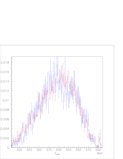
Figure 4: Spectrum of the most energetic photon in the $\phi$ reference frame: left: 2002 data (red histogram) and 2001 data (blue points); right: MC signal $\eta\to 3\gamma$

As can be seen the two distributions for 2001 and 2002 overlap very well. A Kolmogorov test has been performed to check their compatibility, it gives a compatibility probability of 26%, so we use the whole sample. From the distribution is very clear that there isn’t a narrow peak in $E_{max}$, so we don’t see any evidence of $\eta\to 3\gamma$ events.

Then to evaluate the upper limit on the $\eta\to 3\gamma$ signal using this distribution we choose as signal region (the region where there is the main part of the signal) the interval [350,380] MeV. Then we fit the observed distribution of $E_{max}$ in the domain [280,350] MeV $\cup$ [380,480] MeV with a fifth degree polynomial, The fit is good ($\chi^{2}$/n.d.o.f = 77.9/92); (see Fig. 5) and the fitted polynomial is used to estimate the number of the background events in the signal region [350,380].

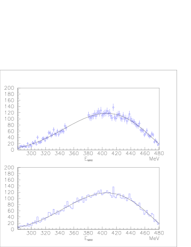
Figure 5: Top: $E_{max}$ distribution for 2001+2002 data. The interval used for background estimation is shown; bottom: the fitted polynomial is overlapped to the whole range.

In this range we assume to have both background and signal and build a likelihood function in this way:

$$Likelihood(N_{sig})=\prod_{i=1}^{N_{bin}}\frac{1}{\sqrt{2\pi N^{exp}_{i}}}\cdot exp-\left[\frac{(N_{i}-N^{exp}_{i})^{2}}{2N^{exp}_{i}}\right]$$

where $N_{i}$ is the number of observed events in the bin “i” (we use in the signal region 15 bins of 1.75 MeV width), and $N^{exp}_{i}$ is the number of the expected events given by:

$$N^{exp}_{i}=a_{1}+a_{2}\cdot x_{i}+a_{3}\cdot x^{2}_{i}+a_{4}\cdot x^{3}_{i}+a_{5}\cdot x^{4}_{i}+a_{6}\cdot x^{5}_{i}+N_{sig}\cdot f_{i}$$

where $x_{i}$ is the central value of the bin “i” and $f_{i}$ is the fraction of signal events that fall in the bin “i” ($\sum_{i}f_{i}=1$). The $f_{i}$ are evaluated using the histogram of Fig. 4(right). The likelihood function and its integral function are shown in Fig. 6. We obtain the following values for the upper limit on $N_{sig}$:

$$N_{sig}\leq 59.0\quad\textrm{at 95 \% C.L.}$$

$$N_{sig}\leq 49.2\quad\textrm{at 90 \% C.L.}\\$$

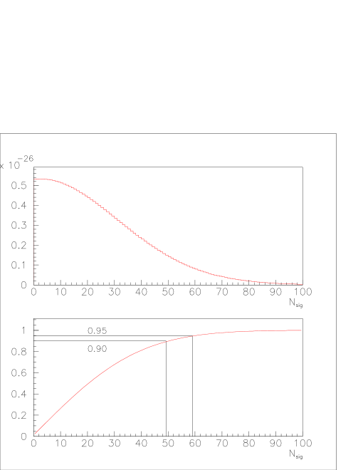
Figure 6: Top: Likelihood as a function of $N_{sig}$; bottom: Integral function of the likelihood; the 95 % and 90 % limits are shown.

To convert the above results into the corresponding upper limits on the Br($\eta\to 3\gamma$) we have evaluated the number of $\eta$ in the data sample through the study of the decay channel $\eta\to 3\pi^{0}$ by using an already developed analysis inside the experiment [9]. The efficiency of the selection evaluated from Monte Carlo is $\epsilon=20.3$ %. The result is: $N(\eta\to 3\pi^{0})=2431917$ and $\epsilon_{\eta\to 3\pi^{0}}=0.4106\pm 0.0016$. Then we evaluate the ratios of the two branching ratios:

$$\frac{Br(\eta\to 3\gamma)}{Br(\eta\to 3\pi^{0})}\leq\frac{N_{Up}~{}\epsilon_{\eta\to 3\pi^{0}}}{N_{\eta\to 3\pi^{0}}~{}\epsilon_{\eta\to 3\gamma}}$$

$$\frac{Br(\eta\to 3\gamma)}{Br(\eta\to 3\pi^{0})}\leq 4.9\cdot 10^{-5}\quad\textrm{95 \% C.L.}$$

$$\frac{Br(\eta\to 3\gamma)}{Br(\eta\to 3\pi^{0})}\leq 4.1\cdot 10^{-5}\quad\textrm{90 \% C.L.}$$

Using the PDG2002 value for $Br(\eta\to 3\pi^{0})=(32.51\pm 0.29)\%$ we have:

$$Br(\eta\to 3\gamma)\leq 1.6\cdot 10^{-5}\quad\textrm{95 \% C.L.}$$

$$Br(\eta\to 3\gamma)\leq 1.3\cdot 10^{-5}\quad\textrm{90 \% C.L.}$$

7 Systematic errors

In this section we evaluate various systematic effects, especially those which may arise from differences between the data and MC distributions used in the analysis.

7.1 Systematics due to the $\chi^{2}cut$

We evaluate the systematics due to possible differences in the $\chi^{2}$ distribution between data and MC by comparing a data control sample with MC. The chosen control sample is the channel $e^{+}e^{-}\to\omega(\to\pi^{0}\gamma)\to 4\gamma$ that is the only channel with four photons that we have in our selection. Since the kinematic fit requires only the energy-momentum conservation, we can compare its $\chi^{2}$ distribution directly to that of the channel $\eta\to 3\gamma$ from MC. We select the $\omega\gamma$ candidates by requiring the mass range $128<m_{\gamma\gamma}<145$ $MeV/c^{2}$ for the $\pi^{0}$ and $760<m_{\pi^{0}\gamma}<815~{}MeV/c^{2}$ for the $\omega$. In Fig. 7 we have reported the $\chi^{2}$ distribution of the kinematic fit, under energy-momentum conservation hypothesis, for the selected $\omega\gamma$ sample and for the MC $\eta\to 3\gamma$ sample. The upper plot is the $\chi^{2}$ distribution, the lower plot is the fraction of events that survives to a given $\chi^{2}$ cut, normalized to the range shown in Fig. For $\chi^{2}_{cut}=25$ the data-MC discrepancy is about 3%. This is the systematic error that we assume for this cut.

Figure 7: Top: $\chi^{2}$ distribution for MC $\eta\to 3\gamma$, continuous line, and $\omega\gamma$ selected sample (see text), dashed line. Bottom: integral of the above distributions.

7.2 Correction for photon detection efficiency

The MC doesn’t simulate with full accuracy the photon detection efficiency, from the study done by [10] we know, as a function of the energy of the photon and the $cos(\theta)$, the ratio $w=\epsilon_{data}/\epsilon_{MC}$. For this reason, we have evaluated the quantity:

$$Weight=\prod_{i=1}^{4}w_{i}\quad\textrm{``i'' runs on the four photons.}$$

for each event. The sum of the weights gives the effect of this discrepancy on the efficiency. The results are:

unweighted events	24376/120000 (20.3 %)
weighted events	24167/120000 (20.1 %)
$\Delta\epsilon/\epsilon$	1.0 %

7.3 Systematics due to signal or background shape and window choice

To test if the kinematic fit introduces a bias in the photon energy that is different for data and MC, we have analyzed a sample of $3\gamma$ events $(\phi\to\eta(\to\gamma\gamma)\gamma)$ and obtained from the kinematic fit the updated energy for every photon. This energy is plotted in Fig. 8 both for data and MC. After having taken in account the wrong $\eta$ mass that we have in MC generator ($m_{\eta}=548.8$ MeV instead of 547.3 MeV) the two distribution overlap very well, so we don’t quote the systematics on this variable.

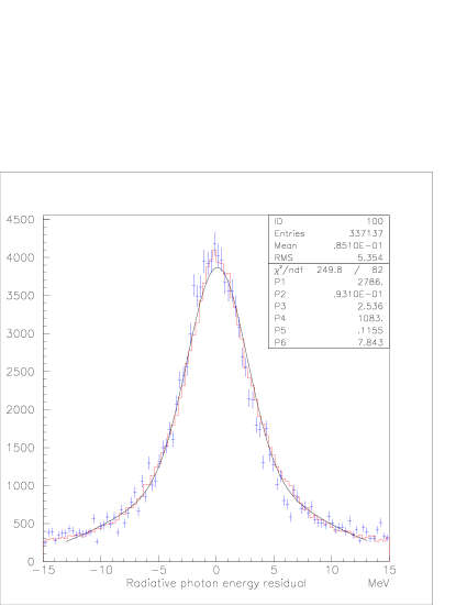
Figure 8: $E_{\gamma}-E_{\gamma rad}$ distribution for photons in the $\phi\to\eta(\to\gamma\gamma)\gamma$ sample. Each event enters three times in the histogram, one for each photon. Both MC (continuous line) and data (points) are shown. $E_{\gamma rad}$ is the expected energy of the radiative photon = 362.7 MeV. The MC shape has been fitted with a double gaussian fit: $P1\cdot exp[-\frac{(x-P2)^{2}}{2\cdot P3^{2}}]+P4\cdot exp[-\frac{(x-P5)^{2}}{2\cdot P6^{2}}]$.

To take into account other possible systematic effects in signal and background shape we varied the width of the signal window and the order of the polynomial used to fit the background shape.Then we repeated the fit of the background (background+signal) excluding (including) the new energy window and by recalculating also the signal efficiency: the maximum variation found on the various upper limit estimates was about 35 $\%$.

8 Conclusions

We have obtained the upper limit $Br(\eta\to 3\gamma)\leq 1.6\cdot 10^{-5}\quad\textrm{at 95 \% C.L.}$ which is significantly better than the PDG existing one and also improves the unpublished Crystal Ball value. We estimate our systematic uncertainties to be at the $35\%$ level. More data to be collected by Kloe in the next future will allow to further improve this result.

References

- [1] S.Guiducci, Status of DANE, in: P. Lucas, S. Webber (Eds.), Proc. of the 2001 Particle Accelerator conference - Chicago, IL U.S.A. (2001)
- [2] D.A. Dicus, Phys. Rev. D 12,2133 (1975)
- [3] B.M.K Nefkens and J.W. Price, Physica Scripta, T99 114,122 (2002)
- [4] K. Hagiwara et al., Phys. Rev. D66, 010001 (2002)
- [5] The KLOE Collaboration, M. Adinolfi et al., Nucl. Instr. and Meth. A488 (2002) 51.
- [6] The KLOE Collaboration, M. Adinolfi et al., Nucl. Instr. and Meth. A482 (2002) 363.
- [7] The KLOE Collaboration, M. Adinolfi et al., Nucl. Instr. and Meth. A483 (2002) 649.
- [8] The KLOE Collaboration, M. Adinolfi et al., Nucl. Instr. and Meth. A492 (2002) 134.
- [9] S.Giovannella, S.Miscetti KLOE note n.177 (2002)
- [10] M.Palutan, T.Spadaro, P.Valente KLOE note n. 174, (2002)