Study of $B^{-}\to D^{**0}\pi^{-}(D^{**0}\to D^{(*)+}\pi^{-})$ decays

Abstract

We report the results of a study of charged $B$ decays to the $D^{\pm}\pi^{\mp}\pi^{\mp}$ and $D^{*\pm}\pi^{\mp}\pi^{\mp}$ final states using complete $D^{(*)}$ reconstruction. The contributions of two-body $B\to D^{**}\pi$ decays with narrow (j=3/2) and broad (j=1/2) $D^{**}$ states have been determined and the masses and widths of four $D^{**}$ states have been measured. This is the first observation of the broad $D^{*0}_{0}$ and $D^{\prime 0}_{1}$ mesons. The analysis is based on a data sample of 65 million $B\bar{B}$ pairs collected in the Belle experiment.

I Introduction

$B$ decays to $D\pi$ and $D^{*}\pi$ final states are two of the dominant hadronic $B$ decay modes and have been measured quite well PDG . In this paper we study the production of $D$-meson excited states, collectively refered to as $D^{**}$’s, that are P-wave excitations of quark-antiquark systems containing one charmed and one light ($u,d$) quark. The results provide tests of Heavy Quark Effective Theory (HQET) and QCD sum rules. Figure 1 shows the spectroscopy of $D$-meson excitations. In the heavy quark limit, the heavy quark spin ${\vec{s}}_{c}$ decouples from the other degrees of freedom and the total angular momentum of the light quark ${\vec{j}}_{q}=\vec{L}+{\vec{s}}_{q}$ is a good quantum number. There are four P-wave states with the following spin-parity and light quark angular momenta: $0^{+}(j_{q}=1/2),~{}1^{+}(j_{q}=1/2),~{}1^{+}(j_{q}=3/2)$ and $2^{+}(j_{q}=3/2)$, which are usually labeled as $D^{*}_{0},~{}D^{\prime}_{1},~{}D_{1}$ and $D^{*}_{2}$, respectively.

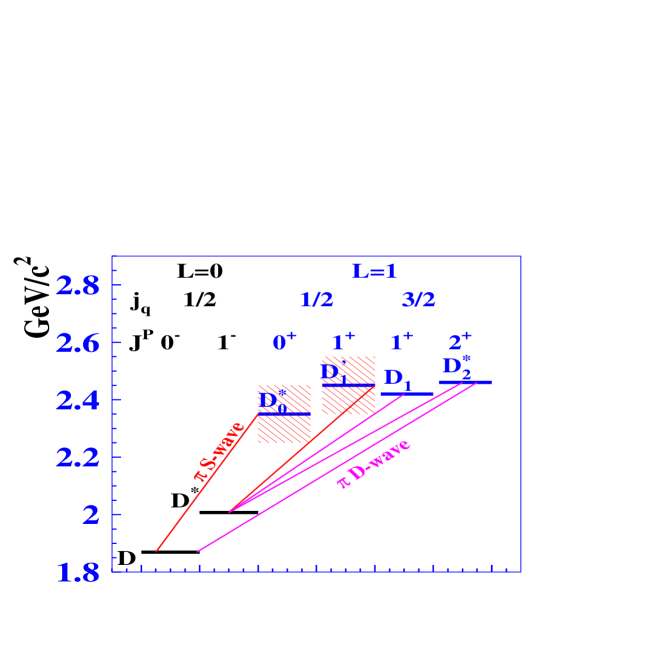
Figure 1: Spectroscopy of $D$-meson excitations. The lines show possible single pion transitions.

The two $j_{q}=3/2$ states are narrow with widths of order 20 MeV and have already been observed AR1 ; AR2 ; AR3 ; e691 ; CL15 ; e687 ; CL2 ; dobs ; DELPHI ; DELPHI1 ; ALEPH . The measured values of their masses agree with model predictions isgur ; rosner ; godfrey ; falk . The remaining $j_{q}=1/2$ states decay via S-waves and are expected to be quite broad. Although they have not yet been directly observed, their total production rate has been measured in $B$-meson semileptonic decays DELPHI .

CLEO has observed the production of both of the narrow $D^{**}$ mesons in $B\to D^{*}\pi\pi$ decays with the following branching fractions CLEO9625 :

$${\cal B}(B^{-}\to D^{0}_{1}\pi^{-})\times{\cal B}(D_{1}^{0}\to D^{*+}\pi^{-}) = (7.8\pm 1.9)\times 10^{-4},$$

$${\cal B}(B^{-}\to D^{*0}_{2}\pi^{-})\times{\cal B}(D_{2}^{*0}\to D^{*+}\pi^{-}) = (4.2\pm 1.7)\times 10^{-4}.$$ (1)

The ratio of the $B$ meson branching fractions

$$R=\frac{{\cal B}(B^{-}\to D^{*0}_{2}\pi^{-})}{{\cal B}(B^{-}\to D^{0}_{1}\pi^{-})}$$ (2)

is calculated in HQET and the factorization approach in Refs. leg ; neubert . In Ref. leg $R$ is found to depend on the values of sub-leading Isgur-Wise functions ($\hat{\tau}_{1,2}$) describing $\Lambda_{QCD}/m_{c}$ corrections. Variations of $\hat{\tau}_{1,2}$ by $\pm 0.75$ GeV result in values of $R$ that range from 0 to 1.5. In Ref. neubert some of the sub-leading terms are estimated and the ratio is determined to be

$$R\approx 0.35\biggl{|}\frac{1+\delta_{8}^{D2}}{1+\delta_{8}^{D1}}\biggr{|}^{2},$$ (3)

where $\delta_{8}^{D1(D2)}$ are non-factorized corrections that are expected to be small. The value of $R$ calculated from the CLEO results given in Eq.(1) plus the ratio of branching fractions ${B(D^{*0}_{2}\to D^{+}\pi^{-})}/{B(D^{*0}_{2}\to D^{*+}\pi^{-})}=2.3\pm 0.8$ CL2 ; AR3 and the assumption that $D_{1}$ and $D_{2}^{*}$ decays are saturated by the two-body $D\pi,~{}D^{*}\pi$ modes, is $R=1.8\pm 0.8$. This value is higher than the prediction, although the uncertainties are large. If more precise measurements do not indicate lower values of $R$, a problem for theory may arise. Thus, a measurement of $R$ will allow us to test HQET predictions.

Another possible inconsistency between theory and experiment is in the ratio of the production rates of narrow and broad states in semileptonic $B$ decays. QCD sum rules QCDSR predict the dominance of narrow $D^{**}$($j_{q}=3/2$) state production in $B\to D^{**}l\nu$ decays. On the other hand, the total branching fraction ${\cal B}(B\to D^{(*)}\pi l^{-}\bar{\nu})=(2.6\pm 0.5)\%$ measured by ALEPH and DELPHI PDG is not saturated by the contribution of the narrow resonances, $(0.86\pm 0.37)\%$ cleol , indicating a large contribution of broad or nonresonant $D^{(*)}\pi$ structures.

In this study we concentrate on charged $B$ decays to $D^{(*)\pm}\pi^{\mp}\pi^{\mp}$. For these decays the final state contains two pions of the same sign that do not form any bound states, making analysis of the final state simpler.

II The Belle detector

The Belle detector Belle is a large-solid-angle magnetic spectrometer that consists of a three-layer silicon vertex detector (SVD), a 50-layer central drift chamber (CDC) for charged particle tracking and specific ionization measurement ($dE/dx$), an array of aerogel threshold Čerenkov counters (ACC), time-of-flight scintillation counters (TOF), and an array of 8736 CsI(Tl) crystals for electromagnetic calorimetry (ECL) located inside a superconducting solenoid coil that provides a 1.5 T magnetic field. An iron flux return located outside the coil is instrumented to detect $K_{L}$ mesons and identify muons (KLM). We use a GEANT-based Monte Carlo (MC) simulation to model the response of the detector and determine the acceptance sim .

Separation of kaons and pions is accomplished by combining the responses of the ACC and the TOF with $dE/dx$ measurements in the CDC to form a likelihood $\cal{L}$($h$) where $h=(\pi)$ or $(K)$. Charged particles are identified as pions or kaons using the likelihood ratio (PID):

$${\rm PID}(K)=\frac{{\cal{L}}(K)}{{\cal{L}}(K)+{\cal{L}}(\pi)};~{}~{}{\rm PID}(\pi)=\frac{{\cal{L}}(\pi)}{{\cal{L}}(K)+{\cal{L}}(\pi)}=1-{\rm PID}(K).$$

At large momenta ($>$2.5 GeV/$c$) only the ACC and $dE/dx$ are used since the TOF provides no significant separation of kaons and pions. Electron identification is based on a combination of $dE/dx$ measurements, the ACC responses and the position, shape and total energy deposition ($E/p$) of the shower detected in the ECL. A more detailed description of the Belle particle identification can be found in ref. PID .

III Event selection

A 60.4 fb^-1 data sample (65.4 million $B\bar{B}$ events) collected at the $\Upsilon(4S)$ resonance with the Belle detector is used. Candidate $B^{-}\to D^{+}\pi^{-}\pi^{-}$ and $B^{-}\to D^{*+}\pi^{-}\pi^{-}$ events as well as charge conjugate combinations are selected. The $D^{+}$ and $D^{*+}$ mesons are reconstructed in the $D^{+}\to K^{-}\pi^{+}\pi^{+}$ and $D^{*+}\to D^{0}\pi^{+}$ modes, respectively. The $D^{0}$ candidates are reconstructed in the $D^{0}\to K^{-}\pi^{+}$ and $D^{0}\to K^{-}\pi^{+}\pi^{+}\pi^{-}$ channels. The signal-to-noise ratios for other $D$ decay modes are found to be much lower and they are not used in this analysis.

Charged tracks are selected with requirements based on the average hit residuals and impact parameters relative to the interaction point. We also require that the polar angle of each track be within the angular range of $17^{\circ}-150^{\circ}$ and that the transverse track momentum be greater than 50 MeV/c for kaons and 25 MeV/c for pions.

Charged kaon candidates are selected with the requirement ${\rm PID}(K)>0.6$. This has an efficiency of $90\%$ for kaons and a pion misidentification probability of $10\%$. For pions the requirement ${\rm PID}(\pi)>0.2$ is used. All tracks that are positively identified as electrons are rejected.

$D^{+}$ mesons are reconstructed from $K^{-}\pi^{+}\pi^{+}$ combinations with invariant mass within 13 MeV/c² of the nominal $D^{+}$ mass, which corresponds to about 3 $\sigma_{K\pi\pi}$. For ${D}^{0}$ mesons, the $K\pi$ or $K\pi\pi\pi$ invariant mass is required to be within 15 MeV/c² of the nominal $D^{0}$ mass (3 $\sigma_{K\pi}$). We reconstruct $D^{*+}$ mesons from the $D\pi$ combinations with a mass difference of $M_{D\pi}-M_{D^{0}}$ within $1.5~{}{\rm MeV}/c^{2}$ of its nominal value.

Candidate events are identified by their center of mass (c.m.) energy difference, $\Delta E=(\sum_{i}E_{i})-E_{\rm b}$, and beam-constrained mass, $M_{\rm bc}=\sqrt{E^{2}_{\rm b}-(\sum_{i}\vec{p}_{i})^{2}}$, where $E_{\rm b}=\sqrt{s}/2$ is the beam energy in the $\Upsilon(4S)$ c.m. frame, and $\vec{p}_{i}$ and $E_{i}$ are the c.m. three-momenta and energies of the $B$ meson candidate decay products. We select events with $M_{\rm bc}>5.20$ GeV/$c^{2}$ and $|\Delta E|<0.10$ GeV.

To suppress the large continuum background ($e^{+}e^{-}\to q\bar{q}$, where $q=u,d,s,c$), topological variables are used. Since the produced $B$ mesons are almost at rest in the c.m. frame, the angles of the decay products of the two $B$ mesons are uncorrelated and the tracks tend to be isotropic while continuum $q\bar{q}$ events tend to have a two-jet structure. We use the angle between the thrust axis of the $B$ candidate and that of the rest of the event ($\Theta_{thrust}$) to discriminate between these two cases. The distribution of $|\cos\Theta_{thrust}|$ is strongly peaked near $|\cos\Theta_{thrust}|=1$ for $q\bar{q}$ events and is nearly flat for $\Upsilon(4S)\to B\bar{B}$ events. We require $|\cos\Theta_{thrust}|<0.8$, which eliminates about 83$\%$ of the continuum background while retaining about 80$\%$ of signal events.

There are events for which two or more combinations pass all the selection criteria. According to a MC simulation, this occurs primarily because of the misreconstruction of a low momentum pion from the $D^{**}\to D^{(*)}\pi$ decay. To avoid multiple entries, the combination that has the minimum difference of $Z$ coordinates at the interaction point, $|Z_{\pi_{1}}-Z_{\pi_{2}}|$, of the tracks corresponding to the pions from $B\to D^{**}\pi_{1}$ and $D^{**}\to D^{(*)}\pi_{2}$ decays is selected foot1 . This selection suppresses the combinations that include pions from $K_{S}$ decays. In the case of multiple $D$ combinations, the one with invariant mass closest to the nominal value is selected.

IV $B^{-}\to D^{+}\pi^{-}\pi^{-}$ analysis

The $M_{\rm bc}$ and $\Delta E$ distributions for $B^{-}\to D^{+}\pi^{-}\pi^{-}$ events are shown in Fig. 2. The distributions are plotted for events that satisfy the selection criteria for the other variable: i.e. $|\Delta E|<25$ MeV and $|M_{\rm bc}-M_{B}|<6$ MeV/c² for the $M_{\rm bc}$ and $\Delta E$ histograms, respectively. A clear signal is evident in both distributions. The signal yield is obtained by fitting the $\Delta E$ distribution to the sum of two Gaussians with the same mean for the signal and a linear function for background. The widths and the relative normalization of the two Gaussians are fixed at values obtained from the MC simulation while the signal normalization as well as the constant term and slope of the background linear function are treated as free parameters.

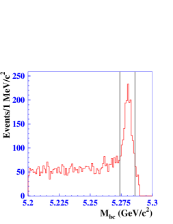
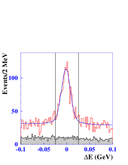
a)	b)

Figure 2: The a) $M_{\rm bc}$ and b) $\Delta E$ distributions for $B^{-}\to D^{+}\pi^{-}\pi^{-}$ events. The hatched histogram in (b) is the $D$ mass sideband ($\big{|}|M_{D}-M_{K\pi\pi}|-26\,\rm MeV/c^{2}\big{|}<6.5\,\rm MeV/c^{2}$).

The signal yield is $1101\pm 46$ events. The detection efficiency of $(18.2\pm 0.2)\%$ is determined from a MC simulation that uses a Dalitz plot distribution that is generated according to the model described in the next section.

Using the branching fraction ${\cal{B}}(D^{+}\to K^{-}\pi^{+}\pi^{+})=(9.1\pm 0.6)\%$ PDG , we obtain

$${\cal B}(B^{-}\to D^{+}\pi^{-}\pi^{-})=(1.02\pm 0.04\pm 0.15)\times 10^{-3},$$

which is consistent with the upper limit obtained by CLEO, ${\cal B}(B^{-}\to D^{+}\pi^{-}\pi^{-})<1.4\times 10^{-3}$ CLEOd . The statistical significance of the signal is greater than 25$\sigma$ foot2 . This is the first observation of this decay mode. The second error is systematic and is dominated by a 10% uncertainty in the track reconstruction (a $2\%$ per track uncertainty was determined by comparing the signals for $\eta\to\pi^{+}\pi^{-}\pi^{0}$ and $\eta\to\gamma\gamma$). The uncertainty in the $D^{+}\to K^{-}\pi^{+}\pi^{+}$ branching fraction is $6.6\%$ and that for the particle identification efficiency is $5\%$. Other contributions are smaller. The uncertainty in the background shape is estimated by adding higher order polynomial terms to the fitting function, which results in less than a $5\%$ change in the branching fraction. The MC simulation uncertainty is estimated to be $3\%$. The possible contribution from charmless $B$-meson decay modes is estimated from the $M_{D}$ sidebands. The sideband distribution, shown as the hatched histogram in Fig. 2(b), indicates no excess from such events in the signal region.

IV.1 $B\to D\pi\pi$ Dalitz plot analysis

For a three-body decay of a spin zero particle, two variables are required to describe the decay kinematics; we use the two $D\pi$ invariant masses. Since there are two identical pions in the final state, we separate the pairs with maximal and minimal $M_{D\pi}$ values.

To analyze the dynamics of $B\to D\pi\pi$ decays, events with $\Delta E$ and $M_{\rm bc}$ within the $|\Delta E|<25$ MeV, $|M_{\rm bc}-M_{B}|<6~{}{\rm MeV}/c^{2}$ signal region are selected. To model the contribution and shape of the background, we use a sideband region defined as 100 MeV $>|\Delta E|>$ 30 MeV with the signal $M_{\rm bc}$ given above. The minimal $D\pi$ mass distributions for the signal and sideband events are shown in Fig. 3, where narrow and broad resonances are visible.

The distributions of events in the $M^{2}_{D\pi~{}min}$ versus $M^{2}_{D\pi~{}max}$ Dalitz plot for the signal and sideband regions are shown in Fig. 4. The Dalitz plot boundary is determined by the decay kinematics and the masses of their daughter particles. In order to have the same Dalitz plot boundary for events in both signal and sideband regions, mass-constrained fits of $K\pi\pi$ to $M_{D}$ and $D\pi\pi$ to $M_{B}$ are performed. The mass-constrained fits also reduces the smearing from detector resolution.

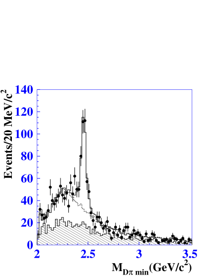
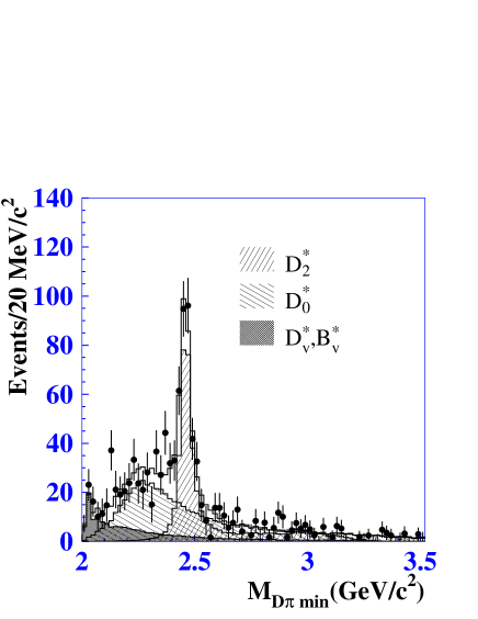
a)	b)

Figure 3: a)The minimal $D\pi$ mass distribution of $B^{-}\to D^{+}\pi^{-}\pi^{-}$ candidates. The points with error bars correspond to the signal box events, while the hatched histogram shows the background obtained from the sidebands. The open histogram is the result of a fit while the dashed one shows the fit function in the case when the narrow resonance amplitude is set to zero. b)The background-subtracted $D\pi$ mass distribution. The points with error bars correspond to the signal box events, hatched histograms show different contributions, the open histogram shows the coherent sum of all contributions.

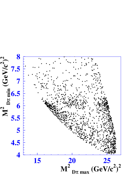
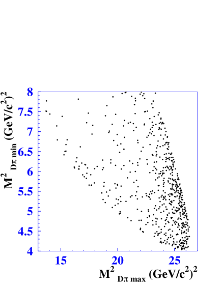
a)	b)

Figure 4: The Dalitz plot for a) signal events and b) sideband events.

To extract the amplitudes and phases of different intermediate states, an unbinned fit to the Dalitz plot is performed using a method similar to CLEO’s CLEODP . The event density function in the Dalitz plot is the sum of the signal and background.

Since the $D\pi$ mass distributions for the upper and lower halves of the $\Delta E$ sideband have similar shapes, we can expect similar background behavior for the signal and sideband regions. The background shape is obtained from an unbinned fit of the sideband distribution to a smooth two-dimensional function. The number of background events in the signal region is scaled according to the relative areas of the signal and the sideband regions.

In the $D^{+}\pi^{-}\pi^{-}$ final state a combination of the $D^{+}$-meson and a pion can form either a tensor meson $D^{*0}_{2}$ or a scalar state $D_{0}^{*0}$; the axial vector mesons $D_{1}^{0}$ and $D^{\prime 0}_{1}$ cannot decay to two pseudoscalars because of the angular momentum and parity conservation. The $D^{*0}$ cannot decay to the $D^{+}\pi^{-}$ because the $D^{*0}$ mass is lower than that of $D^{+}\pi^{-}$. However, a virtual $D^{*}_{v}$ of a higher mass can decay to $D^{+}\pi^{-}$. Another virtual hadron that can be produced in this combination is $B^{*}_{v}$ ($B\to B^{*}_{v}\pi$ and $B^{*}_{v}\to D\pi$). The contributions of these intermediate states are included in the signal-event density ($S(q_{1}^{2},q_{2}^{2})$) parameterization as a coherent sum of the corresponding amplitudes together with a possible constant amplitude ($a_{3}$):

$$S(q_{1}^{2},q_{2}^{2})=\left|a_{D^{*}_{2}}A^{(2)}(q_{1}^{2},q_{2}^{2})+a_{D^{*}_{0}}e^{i\phi_{D^{*}_{0}}}A^{(0)}(q_{1}^{2},q_{2}^{2})+a_{D^{*}_{v}}e^{i\phi_{D^{*}_{v}}}A^{(1)}(q_{1}^{2},q_{2}^{2})+a_{B^{*}_{v}}e^{i\phi_{B^{*}_{v}}}A^{B}(q_{1}^{2},q_{2}^{2})+a_{3}e^{i\phi_{3}}\right|^{2}\otimes{\cal{R}}(\Delta q^{2}),$$ (4)

where $\otimes{\cal{R}}(\Delta q^{2})$ denotes convolution with the experimental resolution. Each resonance is described by a relativistic Breit-Wigner with a $q^{2}$ dependent width and an angular dependence that corresponds to the spins of the intermediate and final state particles:

$$A^{(L)}(q_{1}^{2},q_{2}^{2})=F_{BD^{**}}^{(L)}(\mathbf{p_{1}})\frac{T^{(L)}(q_{1},q_{2})}{q_{1}^{2}-M_{L}^{2}+iM_{L}\Gamma_{L}(q_{1}^{2})}F_{D^{**}D}^{(L)}(\mathbf{p_{2}})+(q_{1}\to q_{2}),$$ (5)

where

$$\Gamma_{L}(q^{2})=\Gamma_{L}\cdot(\mathbf{p_{2}/p_{2}^{0}})^{2L+1}(M_{L}/\sqrt{q^{2}})F_{D^{**}D}^{(L)2}(\mathbf{p_{2}})$$ (6)

is the $q^{2}$ dependent width of the $D^{**}$, with mass $M_{L}$ and width $\Gamma_{L}$, decaying to $D\pi$ state with orbital angular momentum $L$. The variables $p_{1},~{}p_{2},~{}p_{D},~{}q_{1}=p_{2}+p_{D},~{}q_{2}=p_{1}+p_{D}$ are the four-momenta of the pions, $D$, and $D\pi$ combinations, respectively; ${\mathbf{p_{2},~{}p_{2}^{0}}}$ are the magnitude of the pion three-momentum in the $D^{**}$ rest frame when the $D^{**}$ has a four-momentum-square equal to $q^{2}$ and $M_{L}^{2}$, respectively; ${\mathbf{p_{1},~{}p_{1}^{0}}}$ are the magnitude of the pion three-momentum in the $B$ rest frame for the case when the $D^{**}$ four-momentum squared is equal to $q^{2}$ and $M_{L}^{2}$, respectively. The angular dependence for different spins of the intermediate states is:

$$T^{(0)}(q_{1},q_{2})=1,~{}T^{(1)}(q_{1},q_{2})=\frac{M_{B}\mathbf{p_{2}p_{1}}}{\sqrt{q_{1}^{2}}}\cos\theta,~{}T^{(2)}(q_{1},q_{2})=\frac{M_{B}^{2}\mathbf{p_{2}^{2}p_{1}^{2}}}{{q_{1}^{2}}}(\cos^{2}\theta-1/3),$$ (7)

where $\theta$ is the angle between the first pion from the $B$-decay and the pion from the $D^{**}$-decay in the $D^{**}$ rest frame, and $F_{BD^{**}}^{(l)}(\mathbf{p_{1}})$ and $F_{D^{**}D}^{(l)}(\mathbf{p_{2})}$ are transition form factors, which are the most uncertain part of the resonance description. For the $B\to D^{**}$ and $D^{**}\to D$ form factors, we use the Blatt-Weiskopf parameterization blat :

$$F^{(0)}_{AB}(\mathbf{p})=1,~{}F^{(1)}_{AB}(\mathbf{p})=\sqrt{\frac{1+(\mathbf{p^{0}}r)^{2}}{1+(\mathbf{p}r)^{2}}},~{}F^{(2)}_{AB}(\mathbf{p})=\sqrt{\frac{9+3(\mathbf{p^{0}}r)^{2}+(\mathbf{p^{0}}r)^{4}}{9+3(\mathbf{p}r)^{2}+(\mathbf{p}r)^{4}}},$$ (8)

where $r$=1.6 $\rm(GeV/c)^{-1}$ is a hadron scale. For the virtual mesons $D^{*}_{v}$ and $B^{*}_{v}$ that are produced beyond the peak region, another form factor parameterization has been used:

$$F_{AB}(\mathbf{p})=e^{-r(\mathbf{p-p_{0}})};$$ (9)

this provides stronger suppression of the numerator in Eq. (5) far from the resonance region. The resolution function is obtained from MC simulation; the detector resolution for the $D\pi$ invariant mass is about $4$ MeV/$c^{2}$.

The $D^{**}$ resonance parameters ($M_{D^{*0}_{2}},~{}\Gamma_{D^{*0}_{2}},~{}M_{D^{*0}_{0}},~{}\Gamma_{D^{*0}_{0}}$) as well as the amplitudes for the intermediate states and relative phases ($a_{D^{*}_{2}},~{}a_{D^{*}_{v}},~{}a_{D^{*}_{0}},~{}a_{B^{*}},~{}a_{3},~{}\phi_{D^{*}_{v}},~{}\phi_{D^{*}_{0}},~{}\phi_{B^{*}},~{}\phi_{3}$) are treated as free parameters in the fit.

Table 1 gives the results of the fit for different models. When the $D_{v}^{*}$ amplitude is included, the likelihood significantly improves and gives branching fractions values that are consistent with expectation based on the $D^{*}$ width and the $B^{-}\to D^{*0}\pi^{-}$ branching fraction. When the $B^{*}_{v}$ amplitude is added, the likelihood is also significantly improved. A constant phase space term, $a_{3}\exp(i\phi_{3})$, does not substantially change the likelihood and the final results are presented without this term. The variation of the fit parameters when these last amplitudes are included is used as an estimate of the model error.

	I	II		III		IV
Parameters	$D^{*}_{2},~{}D^{*}_{0}$	$D^{*}_{2},~{}D^{*}_{0},D^{*}_{v}$		$D^{*}_{2},~{}D^{*}_{0},D^{*}_{v},~{}B^{*}_{v}$		$D^{*}_{2},~{}D^{*}_{0},D^{*}_{v},~{}B^{*}_{v},$
						ph.sp$(a_{3})$
$Br_{D_{2}^{*}}(10^{-4})$	3.21 $\pm$ 0.24	3.26$\pm$ 0.26		3.38 $\pm$ 0.31		3.47 $\pm$ 0.37
$Br_{D_{0}^{*}}(10^{-4})$	6.09 $\pm$ 0.42	4.96 $\pm$ 0.47		6.12 $\pm$ 0.57		8.35 $\pm$ 0.94
$\phi_{D_{0}^{*}}$	-2.01 $\pm$ 0.10	-2.35 $\pm$ 0.11		-2.37 $\pm$ 0.11		-2.31 $\pm$ 0.14
$Br_{D^{*}_{v}}(10^{-4})$	–	1.46 $\pm$ 0.23		2.21 $\pm$ 0.27		2.23 $\pm$ 0.32
$\phi_{D^{*}_{v}}$	–	0.03 $\pm$ 0.15		-0.25 $\pm$ 0.15		-0.33 $\pm$ 0.19
$Br_{B^{*}_{v}}(10^{-4})$	–	–		0.67 $\pm$ 0.04		0.72 $\pm$ 0.04
$\phi_{B^{*}_{v}}$	–	–		-0.27 $\pm$ 0.28		-0.39 $\pm$ 0.24
$M_{D_{2}^{*0}}(MeV/c^{2})$	2454.6 $\pm$ 2.1	2458.9 $\pm$ 2.1		2461.6 $\pm$ 2.1		2462.7 $\pm$ 2.2
$\Gamma_{D_{2}^{*0}}(MeV)$	43.8 $\pm$ 4.0	44.2 $\pm$ 4.1		45.6 $\pm$ 4.4		46.1 $\pm$ 4.5
$M_{D_{0}^{*0}}(MeV/c^{2})$	2268 $\pm$ 18	2280 $\pm$ 19		2308 $\pm$ 17		2326 $\pm$ 19
$\Gamma_{D_{0}^{*0}}(MeV)$	324 $\pm$ 26	281 $\pm$ 23		276 $\pm$ 21		333 $\pm$ 37
$a_{3}\times 10^{5}$	–	–		–		$0.38\pm 0.65$
$\phi_{3}$	–	–		–		$-0.10\pm 0.93$
$N_{sig}$	1058 $\pm$ 47	1007 $\pm$ 44		1056 $\pm$ 46		1068 $\pm$ 47
$-2\ln\cal{L/L_{0}}$	115	26		0		-7
$\chi^{2}/N$	253.9/129	185.2/127		166.5/125		158.5/123

Table 1: Fit results for different models. The model used to obtain the results includes amplitudes for $D^{*}_{2},~{}D^{*}_{0},D^{*}_{v},~{}B^{*}_{v}$ intermediate resonances. Adding the constant term (ph.sp$(a_{3})$) does not significantly improve the likelihood.

Figure 5 shows the $D\pi$ mass distributions for different $D\pi$ helicity regions. The helicity ($\cos{\theta_{h}}$) is defined as the cosine of the angle between the pions from the $B$ and $D^{**}$ decays in the rest frame of $D^{**}$. The number of events in each bin is corrected for the MC-determined efficiency. The curve shows the fit function for the case when the $D^{*}_{2},~{}D_{0}^{*}$, $D^{*}_{v}$ and $B^{*}_{v}$ amplitudes are included.

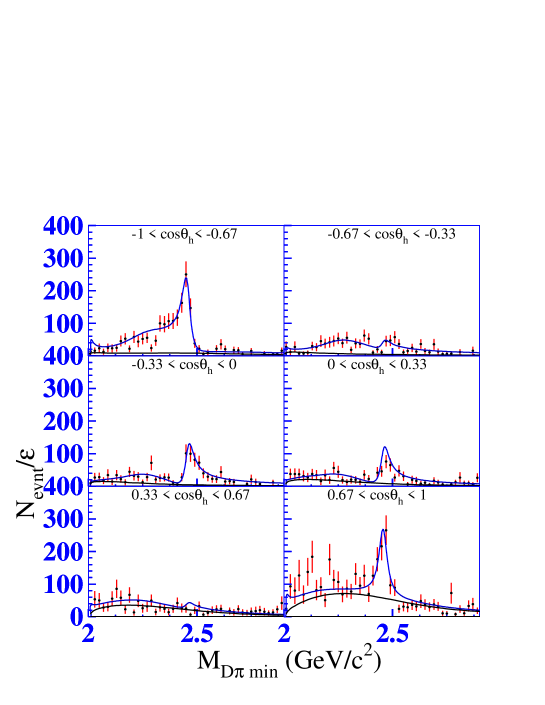
a)                             b)

c)                             d)

e)                             f)

Figure 5: The minimal $D\pi$ mass distribution for different helicity ranges. The two curves are the fit results for the case of $D^{*}_{2},~{}D_{0}^{*}$ and $D^{*}_{v}$ amplitudes (the top curve) and the background contribution (the bottom one). The number of events in each bin is corrected for the efficiency obtained from MC simulation.

The $D^{*}_{2}$ resonance is clearly seen in the helicity range $|\cos\theta_{h}|>0.67$, where the D-wave peaks. The range $0.33<|\cos\theta_{h}|<0.67$ where the D-wave amplitude is suppressed, shows the S-wave contribution from the $D_{0}^{*}$ while the low helicity range $|\cos\theta_{h}|<0.33$ demonstrates a clear interference pattern.

Another demonstration of the agreement between the fitting function and the data is given in Fig. 6, where the helicity distributions for different $q^{2}$ regions are shown. The histogram in the region of the $D^{*}_{2}$ meson clearly indicates a $|\cos^{2}{\theta_{h}}-1/3|^{2}$ D-wave dependence. The distributions in the other regions show reasonable agreement between the fitting function and the data except for a few bins in the small $M_{D\pi~{}min}$ region and with helicity close to 1 (Fig. 6(a)). This region is populated mainly by the virtual $D^{*}_{v}$ and $B^{*}_{v}$ production, the description of which depends on the form factor behavior. This discrepancy does not affect the determination of the $D^{**}$ parameters that are the main topic of this work.

The fit quality is estimated using a two-dimensional histogram of minimum $q^{2}_{D\pi}$ versus the $D\pi$ helicity and calculating the $\chi^{2}/N$ for the function obtained from unbinned likelihood minimization. The confidence level for the model with $D^{*}_{2},~{}D^{*}_{0},~{}D^{*}_{v}$ and $B^{*}_{v}$ is about $0.8\%$. The low confidence level is due to the poor description in the region where $M_{D\pi~{}min}$ is small and $M_{D\pi~{}max}$ is large (or helicity is close to 1) as discussed above.

In Table 2, the likelihood values are presented for the case when the broad scalar resonance is excluded or when it has quantum numbers different from $J^{P}=0^{+}$. For all cases the likelihood values are significantly worse.

Model	$-2\ln({\cal L}/{\cal L}_{max})$
${D^{\star}_{2},~{}D^{\star}_{0},~{}D^{\star}_{v},~{}B^{\star}_{v}}$	0
${D^{\star}_{2},~{}D^{\star}_{v},~{}B^{\star}_{v},}$ ph.sp$(a_{3})$	265
${D^{\star}_{2},~{}D^{\star}_{v}~{},~{}B^{\star}_{v},1^{-}}$	355
${D^{\star}_{2},~{}D^{\star}_{v}~{},~{}B^{\star}_{v},2^{+}}$	235

Table 2: Comparison of models with and without a $0^{+}$ resonance. The amplitudes for $D_{2}^{*}$ and the virtual $D_{v}^{*}$ and $B_{v}^{*}$ are always included.

Thus, we claim the observation of a broad state that can be interpreted as the scalar $D^{*}_{0}$. The fit gives the following parameter values:

$$M_{D^{*0}_{0}}=(2308\pm 17\pm 15\pm 28){\rm MeV}/c^{2},~{}~{}\Gamma_{D^{*0}_{0}}=(276\pm 21\pm 18\pm 60)\rm{MeV}.$$

The values corresponds to the case when four amplitudes (column III of Table 1) were included. Here and throughout the paper the first error is statistical, the second is systematic and the third is the model-dependent error described below.

The values of the narrow resonance mass and width obtained from the fit are:

$$M_{D^{*0}_{2}}=(2461.6\pm 2.1\pm 0.5\pm 3.3){\rm MeV}/c^{2},~{}~{}\Gamma_{D^{*0}_{2}}=(45.6\pm 4.4\pm 6.5\pm 1.6){\rm MeV}.$$

The value of the $D^{*0}_{2}$ width is larger than the world average of $23\pm 5$ MeV, and is consistent with the preliminary result from FOCUS of $30.5\pm 4.2$ MeV e831 . The previous analyses did not take the interference of intermediate states into account; this suggests that there may be large unaccounted systematic errors in these measurements.

The following branching ratio products are obtained:

$${\cal B}(B^{-}\to D^{*0}_{2}\pi^{-})\times{\cal B}(D_{2}^{*0}\to D^{+}\pi^{-})=(3.4\pm 0.3\pm 0.6\pm 0.4)\times 10^{-4},$$

$${\cal B}(B^{-}\to D^{*0}_{0}\pi^{-})\times{\cal B}(D_{0}^{*0}\to D^{+}\pi^{-})=(6.1\pm 0.6\pm 0.9\pm 1.6)\times 10^{-4},$$

and the relative phase of the scalar and tensor amplitude is

$$\phi_{D^{*0}_{0}}=-2.37\pm 0.11\pm 0.08\pm 0.10.$$

The systematic errors are estimated by comparing the fit results for the case when the background shape is taken separately from the lower or upper sideband in the $\Delta E$ distribution. The fit is also performed with more restrictive cuts on $\Delta E$, $M_{\rm bc}$ and $\Delta M_{D}$. The maximum difference is taken as an additional estimate of the systematic uncertainty. For branching fractions, the systematic errors also include uncertainties in track reconstruction and PID efficiency, as well as the error in the $D^{+}\to K^{-}\pi^{+}\pi^{+}$ absolute branching fraction.

The model uncertainties are estimated by comparing fit results for the case of different models (II-IV in Table 1) and for values of $r$ that range from 0 to 5 (GeV/c)^-1 for the transition form factor defined in Eqs. (8) and (9).

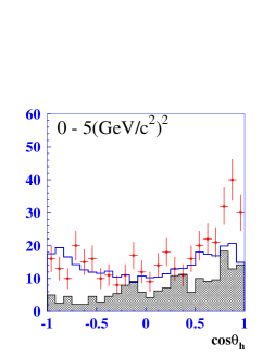
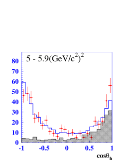
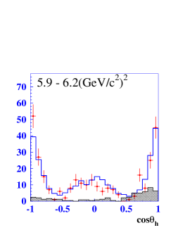
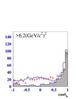
a)	b)
c)	d)

Figure 6: The helicity distribution for data (points with error bars) and for MC simulation (open histogram). The hatched distribution shows the scaled background distribution from the $\Delta E$ sideband region. Figures a), b) correspond to the $q^{2}$ region below $D_{2}^{0}$ resonance, c) – region of the tensor resonance, d) – region higher of the $D_{2}^{0}$.

V $B^{-}\to D^{*+}\pi^{-}\pi^{-}$ analysis

For $D^{*}$ reconstruction, the $D^{*+}\to D^{0}\pi^{+}$ decay is used and two decay modes $D^{0}\to K^{-}\pi^{+}$ and $D^{0}\to K^{-}\pi^{+}\pi^{+}\pi^{-}$ are included. The $\Delta E$ and $M_{\rm bc}$ distributions are shown in Fig. 7. In each mode the number of signal events is obtained in a way similar to that described for the $D\pi\pi$ selection. The observed signal yields of $N_{K\pi}=273\pm 21$ and $N_{K3\pi}=287\pm 22$ for the $K\pi$ and $K\pi\pi\pi$ modes, respectively, are consistent, based on the $D$ branching fractions and the efficiencies determined from MC: $(13.6\pm 0.2)\%$ for $K^{-}\pi^{+}$ and $(6.5\pm 0.2)\%$ for $K^{-}\pi^{+}\pi^{+}\pi^{-}$.

The branching fraction of $(D^{*}\to D\pi)\pi\pi$ events, calculated from the weighted average of the values obtained for the two modes, is:

$${\cal B}(B^{-}\to D^{*+}\pi^{-}\pi^{-})=(1.25\pm 0.08\pm 0.22)\times 10^{-3},$$

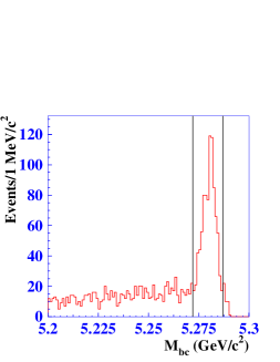
a)	b)

Figure 7: The a) $M_{\rm bc}$ and b) $\Delta E$ distributions for $B^{\mp}\to D^{*\pm}\pi^{\mp}\pi^{\mp}$ candidates.

where the first error is statistical and the second is systematic. This measurement is consistent with the world average value $(2.1\pm 0.6)\times 10^{-3}$ PDG . The systematic error is dominated by the uncertainties in the track reconstruction efficiency $(16\,\%)$ (for a low momentum track from the $D^{*}$ decay the efficiency uncertainty is $8\,\%$) and the PID efficiency $(5\,\%)$. The background shape uncertainty is estimated in the same way as for the $D\pi\pi$ analysis to be $5\%$.

V.1 $B\to D^{*}\pi\pi$ coherent amplitude analysis

In this final state we have a decaying vector $D^{*}$ particle. Assuming the width of the $D^{*}$ to be negligible, there are two additional degrees of freedom and, in addition to two $D^{*}\pi$ invariant masses, two other variables are needed to specify the final state. The variables are chosen to be the angle $\alpha$ between the pions from the $D^{**}$ and $D^{*}$ decay in the $D^{*}$ rest frame, and the azimuthal angle $\gamma$ of the pion from the $D^{*}$ relative to the $B\to D^{*}\pi\pi$ decay plane.

For further analysis, events satisfying the selection criteria described in the first section and having $\Delta E$ and $M_{\rm bc}$ within the $|\Delta E|<30~{}$MeV, $|M_{\rm bc}-M_{B}|<6~{}{\rm MeV}/c^{2}$ signal range are selected. To understand the contribution and shape of the background, we use events in the $100~{}{\rm MeV}>|\Delta E|>30~{}{\rm MeV}$ sideband.

The $D^{*}\pi~{}$ final state can include contributions from the narrow $D_{2}^{*0}$ and $D^{0}_{1}$, and the broad $D^{\prime 0}_{1}$ states. The minimal $D^{*}\pi$ mass distributions for the signal and sideband events are shown in Fig. 8. A narrow structure around $M_{D^{*}\pi}\sim 2.4~{}{\rm GeV}/c^{2}$ and a broader component that can be interpreted as the $D^{\prime}_{1}$ are evident.

The Dalitz plot distributions for the signal and sideband events are shown in Fig. 9. In order to have the same boundary of the Dalitz plot distributions for events from both signal and sideband regions as well as to decrease the smearing effect introduced by the detector resolution, mass-constrained fits of $D\pi$ to $M_{D^{*+}}$ and $D^{*}\pi\pi$ to $M_{B}$ are performed.

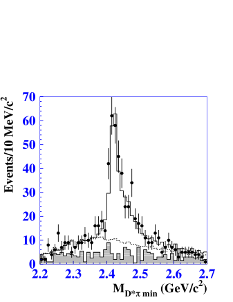
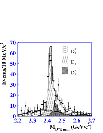
a)	b)

Figure 8: a) The minimal mass distribution of $D^{*}\pi$ events. The points with error bars are experimental data, the hatched histogram is the background distribution obtained from the sideband, the open histogram is MC simulation with the amplitudes and intermediate resonance parameters obtained from the fit. The dashed histogram shows the contribution of the broad resonance. b) The background-subtracted $D^{*}\pi$ mass distribution. The points with error bars correspond to the signal box events, hatched histograms show different contributions, the open histogram is a coherent sum of all contributions.

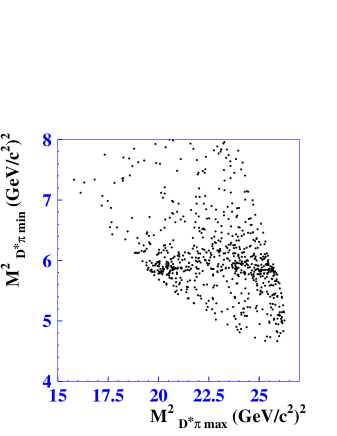
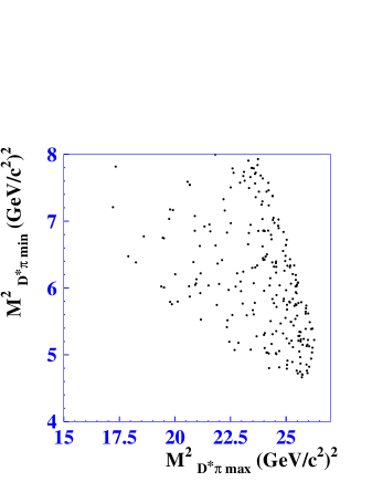
a)	b)

Figure 9: The Dalitz plot for a) signal and b) sideband events.

To extract the amplitudes and phases for different intermediate states, an unbinned likelihood fit in the four-dimensional phase space was performed. Assuming that the background distribution (${\cal B}(q^{2}_{1},q^{2}_{2},\alpha,\gamma)$) in the signal region has the same shape as in the $\Delta E$ sideband, we obtain the ${\cal B}(q^{2}_{1},q^{2}_{2},\alpha,\gamma)$ dependence from a fit of the sideband distribution to a smooth four-dimensional function. The number of background events in the signal region is normalized according to the relative areas of the signal and the sideband regions. The signal is parameterized as a sum of the amplitudes of an intermediate tensor ($D_{2}^{*}$), and two axial vector mesons ($D^{\prime}_{1},~{}D_{1}$) convoluted with the $q^{2}$ resolution function ${\cal{R}}(\Delta q^{2})$ obtained from MC simulation:

$$S(q_{1}^{2},q_{2}^{2},\alpha,\gamma) = \big{|}A^{(D_{1})}(q_{1}^{2},q_{2}^{2},\alpha,\gamma)+A^{(D^{\prime}_{1})}(q_{1}^{2},q_{2}^{2},\alpha,\gamma)+A^{(D_{2}^{*})}(q_{1}^{2},q_{1}^{2},\alpha,\gamma)$$

$$+ a_{D_{v}}e^{i\phi_{D_{v}}}A^{D_{v}}(q_{1}^{2},q_{2}^{2},\alpha,\gamma)+a_{B^{*}_{v}}e^{i\phi_{B^{*}_{v}}}A^{B^{*}}(q_{1}^{2},q_{2}^{2},\alpha,\gamma)+a_{3}e^{i\phi_{3}}\big{|}^{2}\otimes R(\Delta q^{2}).$$

Each resonance is described by a relativistic Breit-Wigner with a width depending on $q^{2}$ (see Eq.5) and angular dependence corresponding to the spins of the intermediate and final state particles.

$$T^{(1D)}(q_{1},q_{2},\alpha,\gamma) = a_{D_{1}}\frac{M_{B}^{2}\mathbf{p_{2}^{2}p_{1}p_{3}}}{\sqrt{q_{1}^{2}}}(\sin\theta\cos\gamma\sin\alpha+2\cos\theta\cos\alpha),$$

$$T^{(1S)}(q_{1},q_{2},\alpha,\gamma) = a_{D^{\prime}_{1}}e^{i\phi_{D^{\prime}_{1}}}\frac{M_{B}\mathbf{p_{1}p_{3}}}{\sqrt{q_{1}^{2}}}(\sin\theta\cos\gamma\sin\alpha-\cos\theta\cos\alpha),$$ (11)

$$T^{(D_{2}^{*})}(q_{1},q_{2},\alpha,\gamma) = a_{D^{*}_{2}}e^{i\phi_{D^{*0}_{2}}}\frac{M_{B}\mathbf{p_{2}^{2}p_{1}^{2}}p_{3}}{\sqrt{q_{1}^{2}}}\cos\theta\sin\theta\sin\alpha\sin\gamma,$$

where $a_{D^{\prime}_{1}},~{}a_{D_{1}},~{}a_{D^{*}_{2}},~{}\phi_{D^{\prime}_{1}},~{}\phi_{D^{*}_{2}}$ are the relative amplitudes and phases for transitions via the corresponding intermediate state. The amplitudes of S and D waves in Eq. (11) correspond to decay via $1^{+}_{1/2}$ and $1^{+}_{3/2}$ intermediate states, respectively. Due to the finite c-quark mass, the observed $1^{+}$ states can be a mixture of pure states. Thus, the resulting amplitude will include a superposition of the amplitudes for the corresponding Breit-Wigner:

$$T^{(D^{\prime}_{1})}(q_{1},q_{2},\alpha,\gamma) = T^{(1S)}(q_{1},q_{2},\alpha,\gamma)\cos\omega-e^{i\psi}T^{(1D)}(q_{1},q_{2},\alpha,\gamma)\sin\omega$$ (12)

$$T^{(D_{1})}(q_{1},q_{2},\alpha,\gamma) = T^{(1S)}(q_{1},q_{2},\alpha,\gamma)\sin\omega+e^{-i\psi}T^{(1D)}(q_{1},q_{2},\alpha,\gamma)\cos\omega.$$

where $\omega$ is the mixing angle and $\psi$ is a complex phase.

The $D^{*}\pi$ pair in the final state can be produced via virtual $D^{0}_{v}$ or $B^{*0}_{v}$ decaying to $D^{*+}\pi^{-}$. Inclusion of a virtual $D_{v}$ significantly improves the likelihood; including in addition $B^{*}_{v}$ and a constant term also improved the likelihood, but the significance is not high (see Table 3).

	$D_{1},~{}D_{2}^{*},~{}D^{\prime}_{1}$	$D_{1},~{}D_{2}^{*},~{}D^{\prime}_{1},D_{v}$		$D_{1},~{}D_{2}^{*},~{}D^{\prime}_{1},~{}D_{v},$		$D_{1},~{}D_{2}^{*},~{}D^{\prime}_{1},~{}D_{v},$
				$B^{*}_{v}$		$B^{*}_{v},$ ph.sp$(a_{3})$
$Br_{D_{1}}(10^{-4})$	7.02 $\pm$ 0.75	6.86 $\pm$ 0.72		6.78 $\pm$ 0.69		6.73 $\pm$ 0.69
$Br_{D_{2}^{*}}(10^{-4})$	1.89 $\pm$ 0.28	2.00 $\pm$ 0.28		1.83 $\pm$ 0.26		1.82 $\pm$ 0.27
$\phi_{D_{2}^{*}}$	-0.53 $\pm$ 0.15	-0.56 $\pm$ 0.14		-0.57 $\pm$ 0.14		-0.56 $\pm$ 0.14
$Br_{D^{\prime}_{1}}(10^{-4})$	5.01 $\pm$ 0.40	4.99 $\pm$ 0.39		4.96 $\pm$ 0.38		4.84 $\pm$ 0.38
$\phi_{D^{\prime}_{1}}$	1.86 $\pm$ 0.18	1.65 $\pm$ 0.23		1.68 $\pm$ 0.20		1.70 $\pm$ 0.20
$Br_{D_{v}}(10^{-4})$	–	0.52 $\pm$ 0.19		0.57 $\pm$ 0.19		0.57 $\pm$ 0.19
$\phi_{D_{v}}$	–	-2.68 $\pm$ 0.26		-2.43 $\pm$ 0.24		-2.43 $\pm$ 0.25
$Br_{B_{v}^{*}}(10^{-4})$	–	–		0.21 $\pm$ 0.10		0.21 $\pm$ 0.11
$\phi_{B_{v}^{*}}$	–	–		1.19 $\pm$ 0.44		1.23 $\pm$ 0.43
$M_{D_{1}^{0}}(MeV/c^{2})$	2421.4 $\pm$ 1.6	2421.2 $\pm$ 1.5		2421.4 $\pm$ 1.5		2421.3 $\pm$ 1.5
$\Gamma_{D_{1}^{0}}(MeV)$	26.7 $\pm$ 3.1	25.2 $\pm$ 2.9		23.7 $\pm$ 2.7		23.5 $\pm$ 2.8
$M_{D^{\prime 0}_{1}}(MeV/c^{2})$	2442 $\pm$ 29	2433 $\pm$ 29		2427 $\pm$ 26		2425 $\pm$ 26
$\Gamma_{D^{\prime 0}_{1}}(MeV)$	454 $\pm$ 100	417 $\pm$ 105		384 ${}^{+107}_{-75}$		374 $\pm$ 87
$\omega$	-0.08 $\pm$ 0.03	-0.09 $\pm$ 0.03		-0.10 $\pm$ 0.03		-0.10 $\pm$ 0.03
$\psi$	0.00 $\pm$ 0.22	0.05 $\pm$ 0.21		0.05 $\pm$ 0.20		0.06 $\pm$ 0.20
$a_{3}\times 10^{4}$	–	–		–		$0.51\pm 0.77$
$\phi_{3}$	–	–		–		$-0.08\pm 0.83$
$N_{sig2}$	277 $\pm$ 21	274 $\pm$ 20		279 $\pm$ 20		278 $\pm$ 20
$N_{sig4}$	275 $\pm$ 20	276 $\pm$ 20		281 $\pm$ 20		281 $\pm$ 20
$-2\ln\cal{L/L_{0}}$	25	7		0		-2

Table 3: Fit results for different models. The model that is used to obtain these results includes amplitudes for $D^{*}_{2},~{}D_{1},~{}D^{\prime}_{1},D_{v},~{}B^{*}_{v}$ intermediate resonances. Adding a constant term does not improve the likelihood significantly.

A fit without the inclusion of a broad resonance gives a considerably worse likelihood (see Table 4). We also tried to fit the data by including a broad resonance with other quantum numbers such as $0^{-},1^{-},~{}2^{+}$. In these cases the likelihood is also significantly worse, as shown in Table 4. We conclude that we have observed the broad $1^{+}$ $D^{\prime}_{1}$ state with a statistical significance of more than 10$~{}\sigma$. The model and systematic errors are estimated in the same way as for the $D\pi\pi$ case.

The $D^{*}_{2}$ mass and width are fixed to the values obtained from the $D\pi\pi$ analysis. The axial vector $D^{**}$ masses and widths as well as the branching fractions and phases of amplitudes $a_{D_{1}},~{}a_{D^{\prime}_{1}},~{}a_{D^{*}_{2}},~{}\phi_{D^{\prime}_{1}},~{}\phi_{D^{*}_{2}}$ are treated as free parameters of the fit as are the mixing angle $\omega$ and the mixing phase $\psi$.

Since there is no good way to graphically present the data and the model in four dimensions, we show the projections of the distributions for various variables. Figure 8 shows the $M_{D^{*}\pi~{}min}$ distribution together with MC results that were generated according to the model containing $D_{1},~{}D^{\prime}_{1},~{}D_{2}^{*}$ and virtual $D_{v},~{}B^{*}_{v}$ intermediate resonances with parameters obtained from the fit. Figure 10 shows a comparison of the data and the MC simulation for $D^{**}$ and $D^{*}$ helicities as well as the angle $\gamma$ for $q^{2}$ ranges corresponding to the two narrow resonances $D_{1}$ ($q^{2}=(5.76\sim 5.98)\rm\,(GeV/c^{2})^{2}$), $D_{2}^{*}$ ($q^{2}=(5.98\sim 6.15)\rm\,(GeV/c^{2})^{2}$) and the regions populated mainly by the broad $D^{\prime}_{1}$ state below ($q^{2}<5.76~{}\rm\,(GeV/c^{2})^{2}$) and above ($q^{2}>6.15~{}\rm\,(GeV/c^{2})^{2}$) the narrow resonances. All distributions indicate good agreement between the data and the fit result. We cannot characterize the quality of the fit by the standard $\chi^{2}$ test since for a binned distribution with four degrees of freedom and a limited data sample any reasonable binning will result in only a few events per bin. Therefore to estimate the quality of the fit we determine $\chi^{2}$ values for different projections of the distributions in Figs. 8 and 10. The obtained $\chi^{2}$ values correspond to confidence levels in the $5-90$ % range.

For the $D_{1}$ meson we obtain the following parameters:

$$M_{D^{0}_{1}}=(2421.4\pm 1.5\pm 0.4\pm 0.8)\,{\rm MeV}/c^{2},~{}\Gamma_{D^{0}_{1}}=(23.7\pm 2.7\pm 0.2\pm 4.0)\,\rm{MeV}.$$

These parameters are in good agreement with the world average values: $M_{D^{0}_{1}}=(2422.2\pm 1.8)\,{\rm MeV}/c^{2},~{}\Gamma_{D^{0}_{1}}=(18.9^{+4.6}_{-3.5})\,\rm{MeV}$ PDG .

The broad $D^{\prime 0}_{1}$ resonance parameters are:

$$M_{D^{\prime 0}_{1}}=(2427\pm 26\pm 20\pm 15)\,{\rm MeV}/c^{2},~{}\Gamma_{D^{\prime 0}_{1}}=(384^{+107}_{-75}\pm 24\pm 70)\,{\rm MeV}.$$

Observation of a similar state was reported by CLEO but was not published; our measurement is consistent with CLEO’s preliminary results: $M_{D^{\prime 0}_{1}}=(2461^{+48}_{-42})\,{\rm MeV}/c^{2},~{}\Gamma_{D^{\prime 0}_{1}}=(290^{+110}_{-90})\,{\rm MeV}$ CLEO996 .

The results for the products of the branching fractions of the $B$ and $D^{**}$ mesons are:

$${\cal B}(B^{-}\to D_{1}\pi^{-})\times{\cal B}(D_{1}\to D^{*+}\pi^{-})=(6.8\pm 0.7\pm 1.3\pm 0.3)\times 10^{-4},$$

$${\cal B}(B^{-}\to D^{*0}_{2}\pi^{-})\times{\cal B}(D_{2}^{*0}\to D^{*+}\pi^{-})=(1.8\pm 0.3\pm 0.3\pm 0.2)\times 10^{-4},$$

$${\cal B}(B^{-}\to D^{\prime 0}_{1}\pi^{-})\times{\cal B}(D^{\prime 0}_{1}\to D^{*+}\pi^{-})=(5.0\pm 0.4\pm 1.0\pm 0.4)\times 10^{-4},$$

the relative phases of the $D^{*}_{2}$ and $D^{\prime}_{1}$ amplitudes are:

$$\phi_{D^{*0}_{2}}=-0.57\pm 0.14\pm 0.06\pm 0.13;~{}\phi_{D^{\prime}_{1}}=1.68\pm 0.20\pm 0.07\pm 0.16,$$

and the mixing angle of two axial states and the complex phase are:

$$\omega=-0.10\pm 0.03\pm 0.02\pm 0.02,$$

$$\psi=0.05\pm 0.20\pm 0.04\pm 0.06.$$

To understand the uncertainties in the background shape and the efficiency of the cuts, additional studies are performed. The background shapes obtained separately for the upper and lower $\Delta E$ sidebands are used in the likelihood optimization. We also apply more restrictive cuts on $\Delta E$ and $M_{\rm bc}$ that improve the signal-to-background ratio by about a factor of two and repeat the fit. The maximum difference between the values obtained with different cuts and different background shapes is included in the systematic error. The branching fraction errors also include an 18% systematic uncertainty in the detection efficiency. The model uncertainties are estimated by comparing fit results for the case of different models (Table 3) and for values of $r$ in the range from 0 to 5 (GeV/c)^-1, where $r$ is the hadron scale parameter in the transition form factors of Eqs. (8) and (9).

Model	$-2\ln\cal{L/L}_{0}$
${D^{\star}_{2},D^{\prime}_{1},D_{1},D_{v},B^{\star}_{v}}$	0
${D^{\star}_{2},D_{1},D_{v},B^{\star}_{v}}$, ph.sp$(a_{3})$	170
${D^{\star}_{2},D_{1},D_{v},B^{\star}_{v},0^{-}}$	107
${D^{\star}_{2},D_{1},D_{v},B^{\star}_{v},1^{-}}$	156
${D^{\star}_{2},D_{1},D_{v},B^{\star}_{v},2^{+}}$	166

Table 4: Comparison of the models with and without a broad $1^{+}$ resonance. The $D_{2}^{*}$ and $D_{1}$ amplitudes are always included.

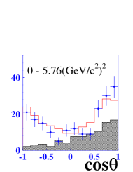
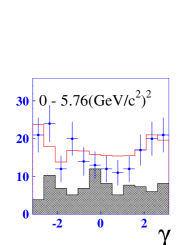
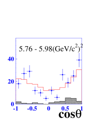
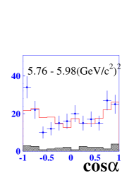
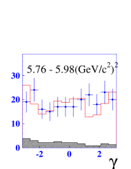
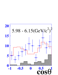
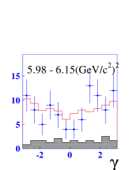
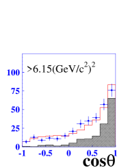
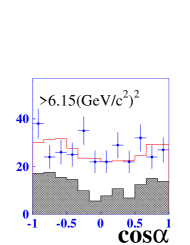
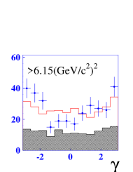
a)	b)	c)
d)	e)	f)
f)	g)	h)
i)	j)	k)

Figure 10: Distributions of the helicity angle of $D^{**}$($\cos\theta$), helicity angle of $D^{*}$($\cos\alpha$) and azimuthal angle $\gamma$ in four different $q^{2}$ regions. The points are the experimental data, the histogram is MC simulation with fitted parameters, the hatched histogram shows the background contribution (from the $\Delta E$ sideband).

VI Discussion

From the measured products of branching fractions of ${\cal B}(B^{-}\to D^{*0}_{2}\pi^{-}){\cal B}(D_{2}^{*0}\to D^{*+}\pi^{-})$ and ${\cal B}(B^{-}\to D^{*0}_{2}\pi^{-}){\cal B}(D_{2}^{*0}\to D^{+}\pi^{-})$ we obtain the ratio of the $D^{*0}_{2}$ branching fractions:

$$H=\frac{{\cal B}(D_{2}^{*0}\to D^{+}\pi^{-})}{{\cal B}(D_{2}^{*0}\to D^{*+}\pi^{-})}=1.9\pm 0.5,$$

which is consistent with the world average $H=2.3\pm 0.6$. Theoretical models rosner ; godfrey ; falk predict $H$ to be in the range from 1.5 to 3. If the $D^{*}_{2}$ decay is saturated by $D\pi$, $D^{*}\pi$ transitions, and $D_{1}$ decay by $D^{*}\pi$, then the ratio $R~{}$ in Eq. (2) can be expressed as the following combination of branching fractions:

$$R=\frac{{\cal B}(B^{-}\to D^{*0}_{2}\pi^{-})({\cal B}(D_{2}^{*0}\to D^{*+}\pi^{-})+{\cal B}(D_{2}^{*0}\to D^{+}\pi^{-}))}{{\cal B}(B^{-}\to D^{0}_{1}\pi^{-}){\cal B}(D_{1}^{0}\to D^{*+}\pi^{-})}=0.77\pm 0.15.$$

The obtained value is lower than that of the CLEO measurement (although the measurements are consistent within errors) but is still a factor of two larger than the factorization result neubert . From our measurement it is impossible to determine whether the non-factorized part for tensor and axial mesons is large, or whether higher order corrections to the leading factorized terms should be taken into account. According to Ref. leg , the observed value of $R$ corresponds to a value of the sub-leading Isgur-Wise function $\hat{\tau}_{1}=0.40^{+0.10}_{-0.15}$ GeV.

For semileptonic decays, where there is no non-factorized contribution, the corresponding ratio is $0.5\pm 0.6$ ALEPH , which, within experimental errors, is consistent with both our measurement and the model prediction. More accurate measurements of semileptonic modes containing $D^{**}$ mesons may help resolve this problem.

Our measurements show that the narrow resonances comprise $(36\pm 6)\,\%$ of $D\pi\pi$ decays and $(63\pm 6)\,\%$ of $D^{*}\pi\pi$ decays. This result is inconsistent with the QCD sum rule QCDSR that predicts the dominance of the narrow states in $B\to D^{(*)}\pi\pi$ decays. It is also possible that in $B^{-}\to D^{**0}\pi^{-}$ decays the color suppressed amplitude is comparable to the tree amplitude, so that other transition form factors play a role. The ratio of the production rates for narrow and broad $D\pi$ states in semileptonic $B\to D^{(*)}\pi l\nu$ decays measured at LEP ALEPH also indicates an excess of the broad states. More accurate measurements of both semileptonic decays and other charged states of the $D^{(*)}\pi\pi$ system may resolve this discrepancy.

VII Conclusion

We have performed a study of charged $B\to D^{+}\pi^{-}\pi^{-}$ and $B\to D^{*+}\pi^{-}\pi^{-}$ decays. The total branching fractions have been measured to be ${\cal B}(B^{-}\to D^{+}\pi^{-}\pi^{-})=(1.02\pm 0.04\pm 0.15)\times 10^{-3}$ and ${\cal B}(B^{-}\to D^{*+}\pi^{-}\pi^{-})=(1.25\pm 0.08\pm 0.22)\times 10^{-3}$. For the former decay this is the first measurement.

A study of the dynamics of these three-body decays is reported. The $D^{+}\pi^{-}\pi^{-}$ final state is well described by the production of $D^{*}_{2}\pi^{-}$ and $D^{*}_{0}\pi^{-}$ followed by $D^{**}\to D\pi$. From a Dalitz plot analysis we obtain the mass, width and product of the branching fractions for the $D^{*0}_{2}$:

$$M_{D^{*0}_{2}}=(2461.6\pm 2.1\pm 0.5\pm 3.3)\,{\rm MeV}/c^{2},~{}\Gamma_{D^{*0}_{2}}=(45.6\pm 4.4\pm 6.5\pm 1.6)\,{\rm MeV},$$

$${\cal B}(B^{-}\to D^{*0}_{2}\pi^{-})\times{\cal B}(D_{2}^{*0}\to D^{+}\pi^{-})=(3.4\pm 0.3\pm 0.6\pm 0.4)\times 10^{-4}.$$

In this mode we also observe production of a broad scalar $D^{*}_{0}$ meson with mass and width:

$$M_{D^{*0}_{0}}=(2308\pm 17\pm 15\pm 28)\,{\rm MeV}/c^{2},\Gamma_{D^{*0}_{0}}=(276\pm 21\pm 18\pm 60)\,{\rm MeV}.$$

The product of the branching fractions for the $D_{0}^{*}$ state is

$${\cal B}(B^{-}\to D^{*0}_{0}\pi^{-})\times{\cal B}(D_{0}^{*0}\to D^{+}\pi^{-})=(6.1\pm 0.6\pm 0.9\pm 1.6)\times 10^{-4},$$

and the relative phase of the scalar and tensor amplitudes is:

$$\phi_{D_{0}^{*0}}=-2.37\pm 0.11\pm 0.08\pm 0.10.$$

This is the first observation of the $D_{0}^{*}$.

The $D^{*}\pi\pi$ final state is described by the production of $D^{*}_{2}\pi$, $D^{\prime}_{1}\pi$ and $D_{1}\pi$ with $D^{**}\to D^{*}\pi$. From a coherent amplitude analysis we obtain the mass, width and product of the branching fractions for the $D_{1}$:

$$M_{D^{0}_{1}}=(2421.4\pm 1.5\pm 0.4\pm 0.8)\,{\rm MeV}/c^{2},~{}\Gamma_{D^{0}_{1}}=(23.7\pm 2.7\pm 0.2\pm 4.0)\,{\rm MeV},$$

$${\cal B}(B^{-}\to D_{1}\pi^{-})\times{\cal B}(D_{1}\to D^{*+}\pi^{-})=(6.8\pm 0.7\pm 1.3\pm 0.3)\times 10^{-4},$$

and measure the product of the branching fractions for the tensor meson process:

$${\cal B}(B^{-}\to D^{*0}_{2}\pi^{-})\times{\cal B}(D_{2}^{*0}\to D^{*+}\pi^{-})=(1.8\pm 0.3\pm 0.3\pm 0.2)\times 10^{-4},$$

and the relative phase of the tensor meson to the axial vector $D^{0}_{1}$:

$$\phi_{D^{*0}_{2}}=-0.57\pm 0.14\pm 0.06\pm 0.13.$$

We observe the broad $D^{\prime}_{1}$ resonance with mass and width:

$$M_{D^{\prime 0}_{1}}=(2427\pm 26\pm 20\pm 15)\,{\rm MeV}/c^{2},~{}\Gamma_{D^{\prime 0}_{1}}=(384^{+107}_{-75}\pm 24\pm 70)\,{\rm MeV}.$$

The product of the branching fractions is:

$${\cal B}(B^{-}\to D^{\prime 0}_{1}\pi^{-})\times{\cal B}(D^{\prime 0}_{1}\to D^{*+}\pi^{-})=(5.0\pm 0.4\pm 1.0\pm 0.4)\times 10^{-4}$$

and the relative phase of $D^{\prime 0}_{1}$ to $D^{0}_{1}$ is:

$$\phi_{D^{\prime}_{1}}=1.68\pm 0.20\pm 0.07\pm 0.16.$$

Our analysis also indicates that the axial vector states mix. The mixing angle is

$$\omega=-0.10\pm 0.03\pm 0.02\pm 0.02,$$

and the phase is

$$\psi=0.05\pm 0.20\pm 0.04\pm 0.06.$$

VIII Acknowledgments

We wish to thank the KEKB accelerator group for the excellent operation of the KEKB accelerator. We acknowledge support from the Ministry of Education, Culture, Sports, Science, and Technology of Japan and the Japan Society for the Promotion of Science; the Australian Research Council and the Australian Department of Industry, Science and Resources; the National Science Foundation of China under contract No. 10175071; the Department of Science and Technology of India; the BK21 program of the Ministry of Education of Korea and the CHEP SRC program of the Korea Science and Engineering Foundation; the Polish State Committee for Scientific Research under contract No. 2P03B 17017; the Ministry of Science and Technology of the Russian Federation; the Ministry of Education, Science and Sport of the Republic of Slovenia; the National Science Council and the Ministry of Education of Taiwan; and the U.S. Department of Energy.

References

(1)K. Hagiwara et al. (Particle Data Group),
Phys. Rev. D 66, 010001 (2002).
(2)
H. Albrecht et al. (ARGUS Collaboration),
Phys. Rev. Lett. 56, 549 (1986).
(3)
H. Albrecht et al. (ARGUS Collaboration),
Phys. Lett. B 221, 422 (1989).
(4)
H. Albrecht et al. (ARGUS Collaboration),
Phys. Lett. B 232, 398 (1989).
(5)
J. C. Anjos et al. (Tagged Photon Spectrometer Collaboration),
Phys. Rev. Lett. 62, 1717 (1989).
(6)
P. Avery et al. (CLEO Collaboration),
Phys. Rev. D 41, 774 (1990).
(7)
P. L. Frabetti et al. (E687 Collaboration),
Phys. Rev. Lett. 72, 324 (1994).
(8)
P. Avery et al. (CLEO Collaboration),
Phys. Lett. B 331, 236 (1994)
[Erratum-ibid. B 342, 453 (1995)].
(9)
T. Bergfeld et al. (CLEO Collaboration),
Phys. Lett. B 340, 194 (1994).
(10)
D. Bloch et al. (DELPHI Collaboration), CERN-OPEN-2000-015,
DELPHI-98-128-CONF-189, Jun 1998. 12pp.
29th International Conference on High-Energy Physics, Vancouver, Canada, 23-29 Jul 1998.
(11)
D. Bloch et al. (DELPHI Collaboration),
DELPHI-2000-106-CONF 405.
(12)
D. Buskulic et al. (ALEPH Collaboration ), Z.Phys. C 73, 601 (1997).
(13)N. Isgur and M.B. Wise, Phys. Rev. Lett. 66, 1130 (1991).
(15)S. Godfrey and R. Kokoski, Phys. Rev. D 43,
1679 (1991).
(16)A.F. Falk and M.E. Peskin, SLAC-PUB-6311 (1993).
(17)J. Gronberg et al. (CLEO Collaboration),
Conference report CLEO CONF 96-25 (1996), contributed paper
to the 28th International conference on High Energy Physics
(ICHEP 96), Warsaw, Poland, July 1996.
(18)A.K. Leibovich, Z. Ligeti, I.W. Stewart, M.B. Wise,
Phys. Rev. D 57, 308 (1997).
(19)M. Neubert, Phys. Lett. B 418, 173 (1998).
(20)A. Le Yaouanc et al., Phys. Lett. B 520, 25 (2001).
(21) J. Anastassov et al. (CLEO Collaboration),
Phys. Rev. Lett. 80, 4127 (1998).
(22)A. Abashian et al. (Belle Collaboration),
Nucl. Instr. and Meth. A 479, 117 (2002).
(23)Events are generated with a modified version of the CLEO group’s QQ program
(http://www.lns.cornell.edu/public/CLEO/soft/QQ); the detector
response is simulated using GEANT, R.Brun et al.,
GEANT 3.21, CERN Report DD/EE/84-1, 1984.
(24)E. Nakano (Belle Collaboration), Proc. of the 8th
International Conference on Instrumentation for Colliding
Beam Physics, Novosibirsk, Russia, 402 (2002).
(25)The coordinate of the track is
defined as the coordinate of the track point closest to the beam in
the
plane. is the axis opposite to the positron beam direction.
(26)
M.S. Alam et al. (CLEO Collaboration),
Phys. Rev. D 50, 43 (1994).
(27)The significance is defined as ,
where is the likelihood with the yield obtained by a fit, and is the likelihood
with the yield constrained to be zero..
(28) S. Kopp et al. (CLEO Collaboration),
Phys. Rev. D 63, 092001 (2001).
(29)J. Blatt and V. Weisskopf, Theoretical Nuclear Physics, p.361,
New York: John Wiley & Sons (1952).
(30)F.L. Fabbri (FOCUS Collaboration), Presented at
ICHEP 2000, Osaka, Japan.
Published in Osaka 2000, High energy physics, vol. 1, 377-380
e-Print Archive: hep-ex/0011044 .
(31)H. Albrecht et al. (ARGUS Collaboration),
Phys. Lett. B 308, 435 (1993).
(32)S. Anderson et al. (CLEO Collaboration),
Conference report CLEO CONF 99-6 (1999).