Phase Motion of the Scalar $\pi\pi$ Amplitudes
in $D^{+}$, $D_{s}^{+}\rightarrow\pi^{-}\pi^{+}\pi^{+}$  Decays

Abstract

We make a direct and model-independent measurement of the low $\pi^{+}\pi^{-}$ mass phase motion in the $D^{+}\to\pi^{-}\pi^{+}\pi^{+}$ decay. Our preliminary results show a strong phase variation, compatible with the isoscalar $\sigma(500)$ meson. This result confirms our previous result prl where we found evidence for the existence of this scalar particle using full Dalitz-plot analysis. We apply the Amplitude Difference (AD) method ad to the same Fermilab E791 data sample used in the preceding analysis. We also give an example of how we extract the phase motion of the scalar amplitude, looking at the $f_{0}(980)$ in $D_{s}^{+}\rightarrow\pi^{-}\pi^{+}\pi^{+}$  decay.

1 Introduction

Fermilab experiment E791, with a full Dalitz plot analysis, showed strong evidence for the existence of light and broad scalar resonances in charm $D^{+}$ meson decay prl ; kappa . The $\pi^{+}\pi^{-}$ resonance is compatible with the isoscalar meson $\sigma(500)$, and was observed in the Cabbibo-suppressed decay $D^{+}\rightarrow\pi^{-}\pi^{+}\pi^{+}$ . To get a good fit quality in this analysis, it was necessary to include an extra scalar particle, other than the well established dipion resonances pdg . For the new state, modeled by a Breit-Wigner amplitude, it was measured a mass and width of $478^{+24}_{-23}\pm 17$ MeV/$c^{2}$ and $324^{+42}_{-40}\pm 21$ MeV/$c^{2}$respectively . The $D^{+}\to\sigma(500)\pi^{+}$ decay contribution is dominant, accounting for approximately half of this particular $D^{+}\rightarrow\pi^{-}\pi^{+}\pi^{+}$  decay. We found also evidence for a scalar $K^{-}\pi^{+}$ resonance, or $\kappa$, in the Cabibbo-allowed decay $D^{+}\rightarrow K^{-}\pi^{+}\pi^{+}$ kappa . Further studies about $\kappa$ are discussed in this proceeding gobel .

In full Dalitz plot analyses, each possible resonance amplitude is represented by a Breit-Wigner function multiplied by angular distributions associated with the spin of the resonance. The various contributions are combined in a coherent sum with complex coefficients that are extracted from maximum likelihood fits to the data. The absolute value of the coefficients are related to the relative fraction of each contribution and the phases take into account the final state interaction (FSI) between the resonance and the third pion.

Due to the importance of this scalar meson in many areas of particle and nuclear physics, it is desirable to be able to confirm the amplitude’s phase motion in a direct observation, without having to assume, a priori, the Breit-Wigner phase approximation for low-mass and broad resonances ochs ; oller ; polosa . Recently, a method was proposed to extract the phase motion of a complex amplitude in three body heavy meson decays ad . The phase variation of a complex amplitude can be directly revealed through the interference in the Dalitz-plot region where it crosses with a well established resonant state, represented by a Breit-Wigner.

Here we begin with a simple example, showing that the AD method can be applied to extract the resonant phase motion of the scalar amplitude due to the resonance $f_{0}(980)$, using the same $f_{0}(980)$ resonance in the crossing channel in the Dalitz plot of the decay $D_{s}^{+}\rightarrow\pi^{-}\pi^{+}\pi^{+}$  using E791 data prlds . This example shows the ability of this method to extract the phase motion of an amplitude. Then we apply the AD method using the well known $f_{2}(1270)$ tensor meson in the crossing channel, as the base resonance, to extract the phase motion of the scalar low mass $\pi\pi$ amplitude in $D^{+}\rightarrow\pi^{-}\pi^{+}\pi^{+}$ , confirming the $\sigma(500)$ suggested by the E791 full Dalitz plot analysis prl .

2 Extracting $f_{0}(980)$ phase motion with the AD method.

From the original $2\times 10^{10}$ event data collected in 1991/92 by Fermilab experiment E791 from $500GeV/c$ $\pi^{-}-nucleon$ interactions ref791 , and after reconstruction and selection criteria, we obtained the $\pi^{-}\pi^{+}\pi^{+}$ sample shown in Figure 1. To study the resonant structure of these three-body decays we consider the 1686 events with invariant mass between 1.85 and 1.89 GeV/c², for the $D^{+}$ analysis and the 937 events with invariant mass between 1.95 and 1.99 GeV/c² for the $D^{+}_{s}$. Figure 2(a) shows the Dalitz-plot for the $D_{s}^{+}\rightarrow\pi^{-}\pi^{+}\pi^{+}$  selected events and Figure 2(b) the Dalitz-plot for $D^{+}\rightarrow\pi^{-}\pi^{+}\pi^{+}$  events. The two axes are the squared invariant-mass combinations for $\pi^{-}\pi^{+}$, and the plot is symmetrical with respect to the two identical pions.

Figure 1: The $\pi^{-}\pi^{+}\pi^{+}$ invariant mass spectrum. The dashed line represents the total background. Events used for the Dalitz analyses are in the hatched areas.

Figure 2: (a) The $D_{s}^{+}\to\pi^{-}\pi^{+}\pi^{+}$ Dalitz plot and (b) the $D^{+}\rightarrow\pi^{-}\pi^{+}\pi^{+}$  Dalitz plot. Since there are two identical pions, the plots are symmetrical.

We can see in Figure 2(a) the scalar $f_{0}(980)$ in $s_{12}$, the square invariant mass, crossing the $f_{0}(980)$ in $s_{13}$, forming an interference region around $s_{13}=s_{12}=$ 0.95GeV². The AD method uses the interference region, between two crossing resonances, to extract the phase motion of one of them, and Final State Interaction (FSI) phase, provided that the second is represented by a Breit-Wigner ad . In fact we are using a Bootstrap approach; that is, using a well established resonance $f_{0}(980)$ in $s_{12}$ to extract its phase motion in $s_{13}$. It is a nice and didactic example to show the ability of this method to extract the phase motion of an amplitude and the FSI phase within the E791 data sample.

The coherent amplitude to describe the crossing between a well known scalar resonance, represented by a Breit-Wigner in $s_{12}$, and a complex amplitude under study in $s_{13}$ in a limited region of the phase space, where we can neglect any other contributions, is given by:

$${\cal A}(s_{12},s_{13})=a_{R}{\cal BW}(s_{12})+a_{s}/(p^{*}/\sqrt{s}_{13})sin\delta(s_{13})e^{i(\delta(s_{13})+\gamma)}$$ (1)

$p^{*}/\sqrt{s}_{13}$ is a phase space factor to make this description compatible with $\pi\pi$ scattering, $\gamma$ is the final state interaction (FSI) phase difference between the two amplitudes, $a_{R}$ and $a_{s}$ are respectively the real magnitudes of the resonance and the under-study complex amplitude. Finally $sin\delta(s_{13})e^{i\delta(s_{13})}$ represents the most general amplitude for a two-body hadronic interaction.

The Breit Wigner distribution is given by:

$${\cal BW}={m_{0}\Gamma_{0}\over{m_{0}^{2}-s-im_{0}\Gamma(m)}}$$

Taking the amplitude square of Equation 1 we get:

$$\mid{\cal A}(s_{12},s_{13})\mid^{2}=a_{R}^{2}\mid{\cal BW}_{f_{0}(980)}(s_{12})\mid^{2}+a_{s}^{2}/p^{*2}/s_{13}\hskip 5.69046ptsin^{2}\delta(s_{13})$$

$$+{2a_{R}a_{s}m_{0}\Gamma_{0}sin\delta(s_{13}){/(p^{*}/\sqrt{s}_{13})}\over(m_{0}^{2}-s_{12})^{2}+m^{2}_{0}\Gamma^{2}(s_{12})}\hskip 2.84544pt\times\hskip 2.84544pt[(m_{0}^{2}-s_{12})cos(\delta(s_{13})+\gamma)+m_{0}\Gamma_{0}sin(\delta(s_{13})+\gamma)]$$ (2)

Since the Breit-Wigner is approximately symmetrical around $m_{0}$ as seen in Figure  3 (the asymmetries would come from $\Gamma(m)$, and is negligible for the narrow $f_{0}(980)$). We can divide our $f_{0}(980)$ mass distribution in two pieces, one for $m_{0}+\epsilon$ and the other with $m_{0}-\epsilon$. From Equation 2 and noticing that the pure Breit-Wigner term will cancel we can write:

Figure 3: $f_{0}(980)$ $s_{12}$ distribution, divided in $m_{0}+\epsilon$ (red) and $m_{0}-\epsilon$ (blue)

$$\mid{\cal A}(m_{0}^{2}+\epsilon,s_{13})\mid^{2}-\mid{\cal A}(m_{0}^{2}-\epsilon,s_{13})\mid^{2}={{-4a_{s}a_{R}/(p^{*}/\sqrt{s}_{13})\epsilon m_{0}\Gamma_{0}\over\epsilon^{2}+m_{0}^{2}\Gamma_{0}^{2}}(sin(2\delta(s_{13})+\gamma)-sin\gamma)}$$ (3)

Only the real part of the interference term in Equation 2 remains.

To extract the phase motion of the scalar amplitude in $s_{13}$ through the $f_{0}(980)$ in $s_{12}$, represented by a Breit-Wigner, we took the events in $s_{12}$ between 0.7 and 1.2 GeV² and divided them into two bins, as presented in Figure  3. The $s_{13}$ distribution for the events of the $s_{12}$ region integrated between 0.95 and 1.2 GeV², is shown in Fig. 4a and the same in Figure 4b for events integrated between 0.7 and 0.95 GeV².

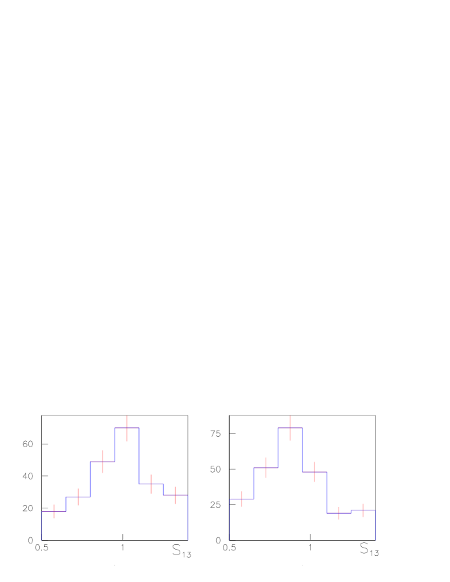
Figure 4: $s_{13}$ distribution. a) For events $\int_{m^{2}_{0}}^{m^{2}_{0}+\epsilon}\mid{\cal A}(s_{12},s_{13})\mid^{2}ds_{12}$. b) For events ${\int_{m^{2}_{0}-\epsilon}^{m^{2}_{0}}\mid{\cal A}(s_{12},s_{13})\mid^{2}ds_{12}}$.

We can see that the peaks in these two plots are in different $s_{13}$ positions. The subtraction of these distributions, corresponds to the integration of Equation 3, that we can write as:

$$\Delta\int{\cal A}^{2}=\int_{m_{eff}^{2}}^{m_{eff}^{2}+\epsilon}\mid{\cal A}(s_{12},s_{13})\mid^{2}ds_{12}-\int_{m_{eff}^{2}-\epsilon}^{m_{eff}^{2}}\mid{\cal A}(s_{12},s_{13})\mid^{2}ds_{12}$$

$$\sim{-{\cal C}(sin(2\delta(s_{13})+\gamma)-sin\gamma)}$$ (4)

where ${\cal C}$ is a constant factor coming from the constant and integrated factors of Equation 3, to be determined from data. The variation of the phase space in the integral was considered negligible for the $f_{0}(980)$ resonance. $\Delta\int{\cal A}^{2}$ directly reflects the behavior of $\delta(s_{13})$. A constant $\Delta\mid{\cal A}\mid^{2}$ would imply constant $\delta(s_{13})$. This would be the case for a non-resonant contribution. The same way a slow phase motion will produce a slowly varying $\Delta\mid{\cal A}\mid^{2}$ and a full resonance phase motion produces a clear signature in $\Delta\mid{\cal A}\mid^{2}$ with the presence of zero, maximum and minimum values.

The subtracted distribution, corresponding to Equation 4, is shown in Figure 5. There is a significant difference between the minimum (bin3) and maximum (bin4) of $\Delta\int{\cal A}^{2}$.

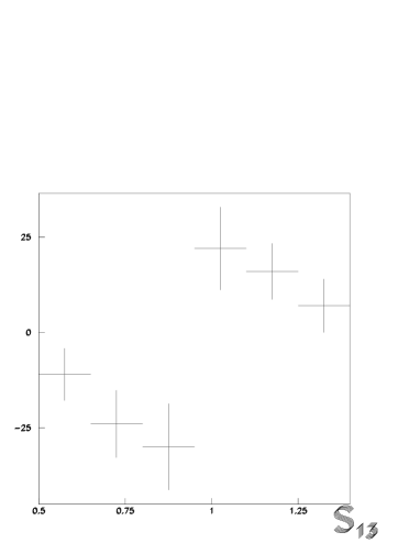
Figure 5: $s_{13}$ distribution of $\Delta\int{\cal A}^{2}ds_{12}$.

We can see in Equation 4 that the zeros occur when $\delta(s_{13})$ = $0^{0}$, $180^{0}$ or $\pi/2-\gamma$. In Figure 5 we can see a zero at $s_{13}$ near 0.5GeV², another one at $s_{13}$ = 0.95GeV² and a third zero near 1.4GeV². Assuming $\delta(s_{13})$ is an analytical function of $s_{13}$, Equation 4 allow us to set the two following conditions at the maximum and minimum values of $\Delta\int{\cal A}^{2}$ respectively:

$$\Delta\int{\cal A}^{2}_{max}\rightarrow sin(2\delta(s_{13})+\gamma)=-1$$ (5)

$$\Delta\int{\cal A}^{2}_{min}\rightarrow sin(2\delta(s_{13})+\gamma)=1$$ (6)

with these two conditions we get ${\cal C}$ and $\gamma$, calculated from the maximum and minimum values of the $\Delta\int{\cal A}^{2}$ distribution in Figure 5:

$${\cal C}=(\Delta\int{\cal A}^{2}_{max}-\Delta\int{\cal A}^{2}_{min})/2$$ (7)

$$\gamma=sin^{-1}({\Delta\int{\cal A}^{2}_{max}+\Delta\int{\cal A}^{2}_{min}\over\Delta\int{\cal A}^{2}_{min}-\Delta\int{\cal A}^{2}_{max}})$$ (8)

From Figure 5 and using the equations above, we measure $\gamma=-0.15\pm 0.31$, that is compatible with zero, as should be since we are crossing the same resonances with, of course, the same final state interaction phase.

With the above conditions we solve Equation 4 for $\delta(s_{13})$:

$$\delta(s_{13})={1\over 2}(sin^{-1}({1\over{\cal C}}\Delta\mid{\cal A}(s_{13})\mid^{2}+sin(\gamma))-\gamma)$$ (9)

Assuming that $\delta(s_{13})$ is an increasing function of $s_{13}$, we can extract directly the $\delta(s_{13})$ value from each bin of Figure 5, creating the $f_{0}(980)$ phase motion shown in Figure 6. The errors in the plot were produced by generating statistically compatible experiments, allowing each bin of $\int_{m^{2}_{0}}^{m^{2}_{0}+\epsilon}\mid{\cal A}(s_{12},s_{13})\mid^{2}$ (Figure4a) and $\int_{m^{2}_{0}-\epsilon}^{m^{2}_{0}}\mid{\cal A}(s_{12},s_{13})\mid^{2}$ (Figure4b) to fluctuate randomly following a Poisson law. We then solve the problem for each ”experiment”. The error in each bin of $\delta(s_{13})$ will be the RMS of the distributions generated by the ”experiments”.

Figure 6: $\delta(s_{13})$ plot with the errors.

From Figure 6 we can see what one could expect, that is the scalar amplitude near 970GeV with a phase motion of about $180^{0}$ degrees. This example demonstrates the ability of AD method to extract the phase motion of an amplitude with E791 statistics.

3 Extracting the scalar low mass $\pi\pi$ amplitude phase motion with the AD method.

In the preceding section, we showed how to apply the AD method to extract the phase motion of an amplitude, from nonleptonic charm-meson three-body decay. Here we apply the same method to extract the phase motion of the scalar low-mass $\pi\pi$ amplitude in $D^{+}\rightarrow\pi^{-}\pi^{+}\pi^{+}$  decay, where we previously found strong experimental evidence for the existence of a light and broad isoscalar resonance prl . To start this analysis, we have to decide what is the best well-known resonance to be used for crossing the low mass amplitude under study. Taking a look at Figure 2b we can see the signature of three resonances that in principle could be used, the $\rho(770)$, $f_{0}(980)$ and $f_{2}(1270)$. In fact, the E791 analysis of this Dalitz plot found a significant contribution from these three resonances in $D^{+}\rightarrow\pi^{-}\pi^{+}\pi^{+}$  decay prl . Since this $D^{+}$ decay is symmetric for the exchange of the $\pi^{+}$ meson, each resonance in $s_{12}$ is present also in $s_{13}$. Then if we use $\rho(770)$ as the base resonance in $s_{12}$, we have also the presence of the $\rho(770)$ in same mass square distribution of the $\sigma(500)$ in $s_{13}$. The proximity of the $\rho(770)$ with the $\sigma(500)$, both broad resonances, creates an overlap between them such that we are not able to separate the phase motion of one from the other. We could use the $f_{0}(980)$ as a base resonance, but again the presence of the $\rho(770)$ overlapping with the $\sigma(500)$ creates the same problem.

There remains only the tensor meson $f_{2}(1270)$ candidate at $m_{0}^{2}=1.61GeV^{2}$, which is placed where the $\rho(770)$ contribution reaches a minimum due the angular distribution in the middle of the Dalitz plot, as we can see from the $D^{+}\to\rho(770)\pi^{+}$ decay Monte Carlo simulation shown in Figure 7.

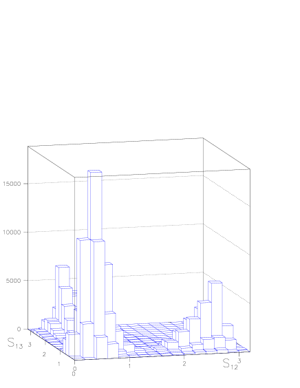
Figure 7: MC $\rho(770)$ distribution in $D^{+}\rightarrow\pi^{-}\pi^{+}\pi^{+}$  decay. There is little contribution between 1.2 to 1.8GeV²

The amplitude for the crossing of the $f_{2}(1270)$ in $s_{12}$ and the complex amplitude under study in $s_{13}$ is given in the same way as in Equation 1:

$${\cal A}(s_{12},s_{13})=a_{R}\hskip 8.5359pt{\cal BW}_{f_{2}(1270)}(s_{12}){\hskip 5.69046pt{}^{j=2}{\cal M}_{f_{2}(1270)}(s_{12},s_{13})}+$$ (10)

$$+\hskip 8.5359pta_{s}/(p^{*}/\sqrt{s}_{13})\hskip 5.69046ptsin\delta(s_{13})\hskip 8.5359pte^{i(\delta(s_{13})+\gamma)}$$

where ${}^{j=2}{\cal M}_{f_{2}(1270)}(s_{12},s_{13})$ is the angular function for the $f_{2}(1270)$ tensor resonance. The amplitude under study represents the scalar low mass $\pi\pi$ amplitude in a limited region of the phase space, where we can neglect the other amplitude contributions.

Both the width $\Gamma(s_{12})$ and the angular function ${}^{j=2}{\cal M}_{f_{2}(1270)}$ from this resonance produce asymmetries in $s_{12}$ and consequently we can not use the nominal $f_{2}(1270)$ mass to divide our sample into two slices, as we did for the $f_{0}(980)$ example. So we performed a Monte Carlo study to determine the effective mass we must use. The $s_{12}$ Monte Carlo projection of the $f_{2}(1270)$ in $D^{+}\rightarrow\pi^{-}\pi^{+}\pi^{+}$  decay is shown in Fig. 8. We can see the asymmetry created around the nominal $f_{2}(1270)$ mass value due to $\Gamma(s_{12})$ and ${}^{j=2}{\cal M}_{f_{2}(1270)}$ contributions to the amplitude.

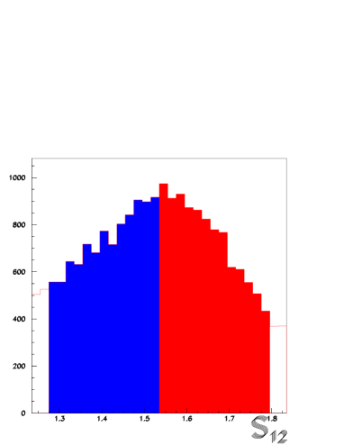
Figure 8: Monte Carlo $f_{2}(1270)$ $s_{12}$ distribution, divided in $m_{0}+\epsilon$ (red) and $m_{0}-\epsilon$ (blue)

Here we require an effective mass squared ($m_{eff}$), such that the number of events integrated between $m_{eff}^{2}$ and $m_{eff}^{2}+\epsilon$ is equal, by construction, to the number of events integrated between $m_{eff}^{2}$ and $m_{eff}^{2}-\epsilon$. We choose, using the $f_{2}(1270)$ Monte Carlo distribution, a mass of $m_{eff}^{2}=1.535GeV^{2}$, within $\pm 0.26GeV^{2}$ , in such way that we can write:

$$\int_{m_{eff}^{2}}^{m_{eff}^{2}+\epsilon}\mid{\cal BW}_{f_{2}(1270)}(s_{12}){{}^{j=2}{\cal M}_{f_{2}(1270)}}\mid^{2}ds_{12}=\int_{m_{eff}^{2}-\epsilon}^{m_{eff}^{2}}\mid{\cal BW}_{f_{2}(1270)}(s_{12}){{}^{j=2}{\cal M}_{f_{2}(1270)}}\mid^{2}ds_{12}$$ (11)

The effective mass squared $m_{eff}$ and the separation between $m_{eff}^{2}+\epsilon$ (red) and $m_{eff}^{2}-\epsilon$ (blue) are shown in Figure 8.

The ${}^{j=2}{\cal M}_{f_{2}(1270)}$ function in $s_{13}$ is presented in Figure 9. The distribution between $m_{eff}^{2}$ and $m_{eff}^{2}+\epsilon$ is shown in Fig. 9a, for events between $m_{eff}^{2}$ and $m_{eff}^{2}-\epsilon$ in Fig. 9b. We can see that these two plots are slightly different. However we considered the approximation ${}^{j=2}{\cal M}^{+}_{f_{2}(1270)}(s_{13})\sim\hskip 2.84544pt^{j=2}{\cal M}^{-}_{f_{2}(1270)}(s_{13})$ and take an average function ${}^{j=2}\bar{\cal M}_{f_{2}(1270)}(s_{13})$. Another important effect, that we had to take into account, is the zero of this function at $s_{13}=0.48GeV^{2}$. Below we discuss the consequences of that in the AD method.

Figure 9: Fast MC ${}^{j=2}{\cal M}_{f_{2}(1270)}$ distribution in $s_{13}$. a) For events between $m_{eff}^{2}$ and $m_{eff}^{2}+\epsilon$. b) For events between $m_{eff}^{2}$ and $m_{eff}^{2}-\epsilon$.

With the above considerations about the $f_{2}(1270)$ in $s_{12}$ and $s_{13}$ we can write the integrated amplitude-square difference as:

$$\Delta\int{\cal A}^{2}=\int_{m_{eff}^{2}}^{m_{eff}^{2}+\epsilon}\mid{\cal A}(s_{12},s_{13})\mid^{2}ds_{12}-\int_{m_{eff}^{2}-\epsilon}^{m_{eff}^{2}}\mid{\cal A}(s_{12},s_{13})\mid^{2}ds_{12}$$

$$\sim{-{\cal C}(sin(2\delta(s_{13})+\gamma)-sin\gamma){\hskip 5.69046pt{}^{j=2}\bar{\cal M}_{f_{2}(1270)}(s_{13})}/(p^{*}/\sqrt{s}_{13})}$$ (12)

This Equation is similar to Equation 4, with an extra angular function term ${}^{j=2}\bar{\cal M}_{f_{2}(1270)}(s_{13})$ .

The background and the acceptance are similar between $m_{eff}^{2}$ and $m_{eff}^{2}+\epsilon$ and $m_{eff}^{2}$ and $m_{eff}^{2}-\epsilon$. Since we are subtracting these two distributions, we do not take into account these effects in our analysis.

The $\int{\cal A}^{2}$ in $s_{13}$, for events integrated in $s_{12}$ between $m_{eff}^{2}=1.535GeV^{2}$ and $m_{eff}^{2}+\epsilon$ and $m_{eff}^{2}$ and $m_{eff}^{2}-\epsilon$, with $\epsilon=0.26GeV^{2}$ are presented in Figure 10a and b respectively.

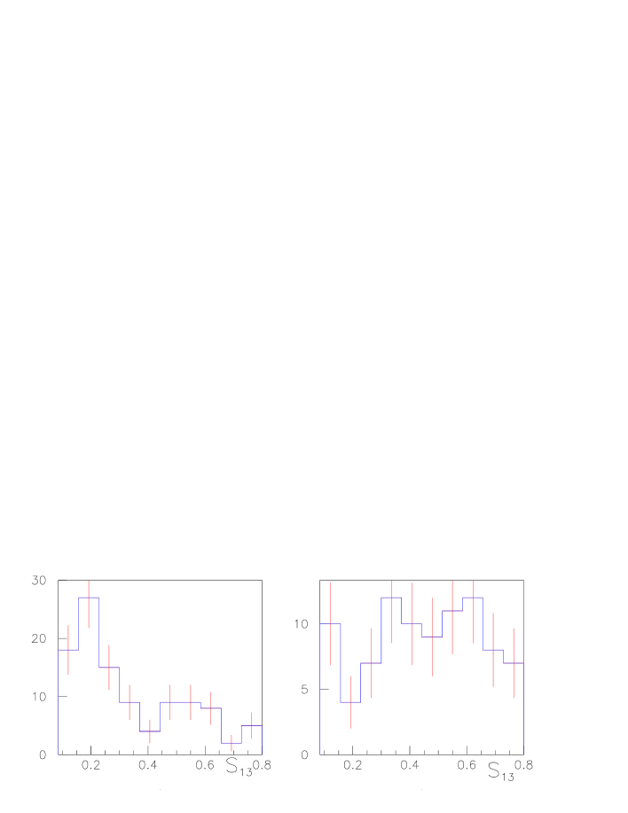
Figure 10: Events distributions in $s_{13}$, a) for events $\int_{m^{2}_{0}}^{m^{2}_{0}+\epsilon}\mid{\cal A}(s_{12},s_{13})\mid^{2}ds_{12}$, b) For events ${\int_{m^{2}_{0}-\epsilon}^{m^{2}_{0}}\mid{\cal A}(s_{12},s_{13})\mid^{2}ds_{12}}$.

Subtracting these two histograms, in the same way we did for the $f_{0}(980)$ example, gives the $\Delta\int{\cal A}^{2}$ of the Equation 12. The result is shown in Figure 11.

Figure 11: $s_{13}$ distribution for $\Delta\int{\cal A}^{2}$.

Here we can not extract directly the phase motion from Figure 11, as we did for the $f_{0}(980)$ example using the conditions 5 and 6. We have to divide the $\Delta\int{\cal A}^{2}$ by $\bar{\cal M}$ (average of the distributions in Figures 9a and b) and multiply by $p^{\prime}$, since phase space here is an important effect. By doing this the only $s_{13}$ dependence of the right hand side of Equation 12 is in $\delta(s_{13})$. However, as we could see in Figure 9, there is a zero about 0.48GeV² in the angular function, which means a singularity around this value in $\Delta\int{\cal A}^{2}/\bar{\cal M}$. To avoid this singularity, we first produced a binning in such a way that the singularity is placed in the middle of one bin. In Figure 12 we show the $\Delta\int{\cal A}^{2}$ by $\bar{\cal M}$ distribution. We can see that the 6th bin (around 0.48GeV²), has a huge error, that corresponds to the bin of the singularity. Due to the singularity we decided not to use this region (bin 6) further in this analysis. The consequences of this choice are going to be taken care of in systematic error studies. In any case, the singularity could only affect the position of the minimum of Figure 12. It does not interfere with the general feature of starting at zero, having statistically significant maximum and minimum values, and coming back to zero, indicating a strong phase variation. Bins 2 and 5 are respectively the maximum and minimum value of $\Delta\int{\cal A}^{2}p^{\prime}/\bar{\cal M}$ of Figure 12 where we use the Equation 5 and 6 conditions.

Figure 12: $s_{13}$ distribution for $\Delta\int{\cal A}^{2}\hskip 2.84544ptp^{\prime}/\bar{\cal M}$.

With the same assumptions used for the $f_{0}(980)$, that is $\delta(s_{13})$ is an analytical and increasing function of $s_{13}$, and using Equation 7, 8 and 9 (multiplied by $p^{\prime}$ and divided by $\bar{\cal M}$), we can extract $\gamma$ and $\delta(s_{13})$ from Figure 12. For the FSI phase we found $\gamma=3.26\pm 0.33$, that is somewhat bigger than found by the E791 full Dalitz-plot analysis prl ($\gamma_{Dalitz}=2.59\pm 0.19$). The fact that we used the effective mass for the $f_{2}(1270)$ = 1.535 GeV² instead of the nominal mass is responsable for the shift observed in the relative phase. To verify this statement we generated 1000 samples of fast-MC, with only two amplitudes, $f_{2}(1270)$ and $\sigma(500)$. For both we used Briet-Wigner functions and the E791 parameters. We generated the phase difference of 2.59 rad, measured by the E791. For these 1000 samples, we measure $\gamma$ using the method presented here. The result has a mean value of 3.07. We can say that the difference between the generated and measured $\gamma$ value is a correction factor due to the use of an effective mass. Using this offset factor ( 2.59 - 3.07 = -0.48) we correct the measurement $\gamma=3.26\pm 0.33$ to $\gamma_{corr}=2.78\pm 0.33$. So the observed $\gamma$ difference between Dalitz analysis and the $\gamma_{corr}$ is in good agreement, with a difference below one standard deviation.

The $\delta(s_{13})$ was extracted bin by bin, with the same approach for the errors used in the $f_{0}(980)$ example, and we got the distribution shown in Figure 13 . We can see a strong phase variation of about 180⁰ around the mass for the $\sigma(500)$, showing a phase motion compatible with a resonance.

Figure 13: Phase motion $\delta(s_{13})$ distribution for the scalar low mass $\pi\pi$ amplitude, with the errors.

4 Conclusions

We showed that the AD method can be applied to E791 data to extract the phase motion of the resonance $f_{0}(980)$ in the Dalitz plot of the decay $D_{s}^{+}\rightarrow\pi^{-}\pi^{+}\pi^{+}$ . This example demonstrates the ability of this method to extract the phase motion of a resonance amplitude.

Preliminary E791 results present a direct and model-independent approach, obtained with the AD method, and confirms our previous result of the evidence of an important contribution of the isoscalar $\sigma(500)$ meson in $D^{+}\rightarrow\pi^{-}\pi^{+}\pi^{+}$  decay prl . We use the well known $f_{2}(1270)$ tensor meson in the crossing channel, as the base resonance, to extract the phase motion of the low mass $\pi\pi$ scalar amplitude. We obtain a $\delta(s_{13})$ variation of about 180⁰ consistent with a resonant $\sigma(500)$ contribution. We also obtain good agreement between the FSI $\gamma_{corr}$ observed with AD method and the $\gamma$ observed in the full Dalitz plot analysis.

References

- (1) E791 Collaboration, E.M. Aitala et al., Phys. Rev. Lett. 86, 770 (2001).
- (2) I. Bediaga and J. Miranda, Phys. Lett. B550, 135 (2002).
- (3) E791 Collaboration, E.M. Aitala et al., Phys. Rev. Lett. 89, 121801 (2002).
- (4) Particle Data Group, Hagiwara et al., Phys. Rev. D 66, 010001-1 (2002).
- (5) Carla Göbel for E791 collaboration, this proceeding and hep-ex/0307003.
- (6) Peter Minkowski and Wolfgang Ochs, hep-ph/0209225. To be appear in the proceeding of QCD 2002 Euroconference, Montpellier 2-9 July 2002.
- (7) J. A. Oller, hep-ph/0306294. To be appear in the proceeding of Workshop on the CKM Unitarity Triangle, IPPP Durham, April 2003.
- (8) A. D. Polosa, hep-ph/0306298. To be appear in the proceeding of Workshop on the CKM Unitarity Triangle, IPPP Durham, April 2003.
- (9) E791 Collaboration, E.M. Aitala et al., Phys. Rev. Lett. 86, 765 (2001).
- (10) J.A. Appel, Ann. Rev. Nucl. Part. Sci. 42, 367 (1992); D. Summers et al., hep-ex/0009015; S. Amato et al., Nucl. Instr. Meth. A 324, 535 (1993); E.M. Aitala et al., Eur. Phys. J. direct C1, 4 (1999); S. Bracker et al., hep-ex/9511009. S. Bracker and S. Hansen, hep-ex/0210034, S. Hansen et al., IEEE Trans. Nucl. Sci. 34, 1003 (1987).