The scalar $\kappa$ from $D^{+}\to K^{-}\pi^{+}\pi^{+}$:
Further Studies

Abstract

We briefly review the recent results obtained by Fermilab experiment E791 on the Dalitz plot analysis of the decay $D^{+}\to K^{-}\pi^{+}\pi^{+}$, where indication for a light $K\pi$ scalar resonance, the $\kappa$, was found. We also present preliminary studies providing further information on the phase behavior of the scalar components at low mass, supporting the previous indication for the $\kappa$.

1 INTRODUCTION

Nowadays, with the rising statistics of charm samples, the decays of charm mesons can be seen as a new source for the study of light meson spectroscopy, complementary to that from scattering experiments, and can be particularly relevant to the understanding of the scalar sector.

Recently, Fermilab experiment E791 reported on the indication of a light scalar $K\pi$ resonance dkpipi , $\kappa$, based on a full Dalitz plot analysis of the decay $D^{+}\to K^{-}\pi^{+}\pi^{+}$. The measured Breit-Wigner mass and width of this state were found to be $797\pm 19\pm 43$ MeV/c² and $410\pm 43\pm 87$ MeV/c², respectively. Fermilab E791 has also observed evidence for the scalar $\sigma$ meson in $D^{+}\to\pi^{-}\pi^{+}\pi^{+}$ decays d3pi and measured $f_{0}$ masses and widths in $D_{s}^{+}\to\pi^{-}\pi^{+}\pi^{+}$ decays ds3pi .

Here, we briefly review the $D^{+}\to K^{-}\pi^{+}\pi^{+}$ methodology and the results obtained. Moreover, we present new, preliminary studies providing further information on the phase variation of the scalar sector at low mass. We first present a study of the interference of $K^{*}(890)$ and underlying amplitudes as an attempt to measure the phase motion of the scalar low-mass $K\pi$ amplitude. A more extensive study comes afterwards, where we try a set of fit models inspired by the LASS parametrization for the S-wave $K\pi$ amplitude lass . The main idea is to check whether a unitary, isolated, S-wave $K\pi$ amplitude can fit the $D^{+}\to K^{-}\pi^{+}\pi^{+}$ Dalitz plot, together with the other (higher-spin) intermediate states. We show that this approach is not adequate for the data, and present similar parametrizations where final-state interactions are included for the S-wave components, as is usually done in Dalitz plot analyses. In particular, we present a result offering further support for a rapidly-varying phase at low $K\pi$ mass, consistent with the previous indication of a light, broad $\kappa$ in $D^{+}\to K^{-}\pi^{+}\pi^{+}$.

2 REVIEW OF THE $D^{+}\to K^{-}\pi^{+}\pi^{+}$ RESULTS

From the original $2\times 10^{10}$ events collected by Fermilab E791 e791 , and after reconstruction and selection criteria, we obtained the $K^{-}\pi^{+}\pi^{+}$ mass spectrum shown in Fig.1(a). The sample of 15,090 events shown in the crosshatched area is used for the Dalitz plot analysis of $D^{+}\to K^{-}\pi^{+}\pi^{+}$, from which about 6% is due to background. The Dalitz plot of these events are shown in Fig.1(b), where the axes represent the two invariant mass squared combinations $s_{12}$ and $s_{13}$ (the kaon is labeled particle 1, the two pions are particles 2 and 3).

For the Dalitz plot analysis, an unbinned maximum-likelihood fit was performed with probability distribution funtions (PDF’s) for both signal and background. The signal PDF was written as the square of the total physical amplitude ${\cal A}$ and it is weighted by the acceptance across the Dalitz plot and by the level of signal to background for each event.

Many $K^{*}$ resonances could contribute to the final state by forming quasi 2-body intermediate states $\bar{K}^{*}\pi^{+}$, as well as a possible non-resonant (NR) 3-body decay. Due to the possibility of rescattering of these intermediate states from final state interactions (FSI), a general ansatz, widely use in Dalitz analyses of $D$ decays to describe the total decay amplitude, is given by

$${\cal A}=a_{\rm NR}e^{i\delta_{\rm NR}}{\cal A}_{\rm NR}+\sum_{n=1}^{N}a_{n}e^{i\delta_{n}}{\cal A}_{n}~{}.$$ (1)

This equation uses Lorentz invariant amplitudes ${\cal A}_{n}$ to describe the individual resonant and NR processes, with relative strenghts given by the magnitudes $a_{n}$ and strong phases $\delta_{n}$ to account for FSI. The NR amplitude ${\cal A}_{\rm NR}$ is usually assumed constant and set to 1. The resonant amplitudes are written as ${\cal A}_{n}=\ BW_{n}~{}F_{D}^{(J)}~{}F_{n}^{(J)}~{}{\cal M}_{n}^{(J)}$ where $BW_{n}$ is the relativistic Breit-Wigner propagator, $BW_{n}=\left[m^{2}_{0}-m^{2}-im_{0}\Gamma(m)\right]^{-1}$, the quantities $F_{D}$ and $F_{R}$ are the Blatt-Weisskopf damping factors respectively for the $D$ and the $K\pi$ resonances and ${\cal M}_{n}^{(J)}$ describes the angular function according to the spin $J$ of the resonance. See dkpipi . The amplitudes are generally functions of both Dalitz variables $s_{12}$ and $s_{13}$. Here, with two identical pions in the final state, each amplitude is Bose symmetrized ${\cal A}_{n}={\cal A}_{n}[({\bf 12}){\bf 3}]+{\cal A}_{n}[({\bf 13}){\bf 2}]$.

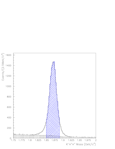
(a)

(b)

Figure 1: (a) The $K\pi\pi$ invariant mass spectrum. The filled area is background; (b) Dalitz plot corresponding to the events in the crosshatched area of (a).

The first approach to fit the data includes the known $K^{*}$ resonances plus a constant NR term. This is called Model A. It finds contributions from the channels: NR, with a decay fraction over 90%, followed by $\bar{K}^{*}_{0}(1430)\pi^{+}$, $\bar{K}^{*}(892)\pi^{+}$, $\bar{K}^{*}(1680)\pi^{+}$ and $\bar{K}^{*}_{2}(1430)\pi^{+}$; these values are in accordance with previous results from Fermilab E691e691-kpipi and Fermilab E687e687-kpipi . See fit fractions and relative phases in Table 1. There is an important destructive interference pattern, since all fractions add up to 140%. Important disagreements appear between the fit to Model A and data, with $\chi^{2}/\nu=2.7$ ($\nu$ being the number of degrees of freedom) in a binned version of the Dalitz plot. The discrepancies are found mainly at low $K\pi$ mass squared (below 0.8 ${\rm GeV^{2}/c^{4}}$) and near 2.5 ${\rm GeV^{2}/c^{4}}$ dkpipi . Thus, a model with the known $K\pi$ resonances, plus a constant NR amplitude, is not able to describe the $D^{+}\to K^{-}\pi^{+}\pi^{+}$ Dalitz plot satisfactorily.

A second model (Model B) allows the mass and width of the scalar $K^{*}_{0}(1430)$ to float, and includes Gaussian form-factors dkpipi . The resulting fractions and phases are similar to those of Model A (within errors) and the mass and width of $K^{*}_{0}(1430)$ are found to be consistent with PDG values. The fit improves but it is still unsatisfactory.

A third fit model, Model C, is constructed by the inclusion of an extra scalar state, with unconstrained mass and width. The mass and width of the $K^{*}_{0}(1430)$ are also free parameters, and Gaussian form-factors are used as in Model B. Using this model, the values obtained are $797\pm 19\pm 43$ MeV/c² for the mass and $410\pm 43\pm 87$ MeV/c² for the width of the new scalar state, here referred to as the $\kappa$. The values of mass and width obtained for the $K^{*}_{0}(1430)$ are respectively $1459\pm 7\pm 5$ MeV/c² and $175\pm 12\pm 12$ MeV/c², appearing heavier and narrower than presented by the PDG. The fit fractions and phases from Models C are shown in Table 1. Compared to the results of Model A (without $\kappa$), the NR mode drops from over 90% to 13%. The $\kappa\pi^{+}$ state is now dominant, with a decay fraction about 50%. Moreover, the fit quality of Model C is substantially superior to that of Model A; the $\chi^{2}/\nu$ is now 0.73.

Table 1: Results without $\kappa$ (Model A) and with $\kappa$ (Model C).

Decay	Model A: No $\kappa$		Model C: With $\kappa$
Mode	Fraction (%)	Phase	Fraction (%)	Phase
NR	$90.9\pm 2.6$	$0^{\circ}$ (fixed)	$13.0\pm 5.8\pm 4.4$	$(-11\pm 14\pm 8)^{\circ}$
$\kappa\pi^{+}$	–	–	$47.8\pm 12.1\pm 5.3$	$(187\pm 8\pm 18)^{\circ}$
$\bar{K}^{*}(892)\pi^{+}$	$13.8\pm 0.5$	$(54\pm 2)^{\circ}$	$12.3\pm 1.0\pm 0.9$	$0^{\circ}$ (fixed)
$\bar{K}^{*}_{0}(1430)\pi^{+}$	$30.6\pm 1.6$	$(54\pm 2)^{\circ}$	$12.5\pm 1.4\pm 0.5$	$(48\pm 7\pm 10)^{\circ}$
$\bar{K}^{*}_{2}(1430)\pi^{+}$	$0.4\pm 0.1$	$(33\pm 8)^{\circ}$	$0.5\pm 0.1\pm 0.2$	$(-54\pm 8\pm 7)^{\circ}$
$\bar{K}^{*}(1680)\pi^{+}$	$3.2\pm 0.3$	$(66\pm 3)^{\circ}$	$2.5\pm 0.7\pm 0.3$	$(28\pm 13\pm 15)^{\circ}$

From the results of the Dalitz plot analysis of $D^{+}\to K^{-}\pi^{+}\pi^{+}$, one concludes that a conventional approach, including known $K\pi$ resonances and a constant NR term, cannot describe the data. The presence of a broad, light scalar $K\pi$ state, $\kappa$, provides a very good description of the data and becomes the major contribution to the decay. Many other possibilities were tried with no sucess, for instance a toy model for which the extra state is represented by a Breit-Wigner without phase variation, vector and tensor hypotheses, different parametrizations for the NR channel, etc.

3 Further Studies

As described above, we obtain a very good description of the $D^{+}\to K^{-}\pi^{+}\pi^{+}$ data by the inclusion of the $\kappa$ in the decay amplitude. A scalar resonant phase behavior seems to be required at low mass. Nevertheless, it is desirable to investigate further, and independently of the Breit-Wigner hypothesis.

Here, we present new studies in order to provide further information on the phase behavior of the scalar amplitude at low mass. A first study refers to the asymmetry of the $K^{*}(890)$ and we show that there is no sensivity to the $\kappa$ phase motion at the $K^{*}(890)$ mass in the crossed channel, although an indication of it can be seen at lower and higher mass. A second, more important study, refers to a comparison with the results of the S-wave $K\pi$ amplitude from LASS, composed of a non-resonant background (with effective range parametrization) and the $K^{*}_{0}(1430)$. The main results we obtain are the inability to describe the data by imposing a $K\pi$ elastic unitarity constraint but, on the other hand, the features of the phase motion obtained after this imposition is released.

3.1 $K^{*}(890)$ Asymmetry Study

A suggestion has been made to us ochsprivate to see whether the phase motion of the $\kappa$ could be inferred through the interference of the $K^{*}(890)$ with the broad, underlying amplitude. From Fig.1(a) a strong asymmetry in the interference of the $K^{*}(890)$ is evident in the Dalitz plot. This asymmetry is due to the interference with the dominant scalar component at low mass, i.e., the NR component in Model A (without $\kappa$) or the broad $\kappa$ in Model C. In the following, we will explore this possibility.

If one plots the phase of the $\kappa$ Breit-Wigner ($\delta_{BW}$) with central mass and width obtained by E791 (797 MeV/c² and 410 MeV/c², respectively) one sees that there is a sharp increasing of the phase from threshold up to about 1 GeV/c² (see Fig.2). Above 1 GeV/c², the increase is slow. Now, we want to study the $\kappa$ phase motion in $m_{13}$ by inspection of the $\cos\theta_{V}$ distribution of $K^{*}(890)$ ($\theta_{V}$ being the decay angle of the $K$ in the center-of-mass frame of $K^{*}(890)$ with respect to the $D$ direction) within 0.8 and 1.0 GeV/c² in the crossed channel, $m_{12}$. By observing the Dalitz Plot, we see that for $0.8<m_{12}<1.0$ GeV/c², the allowed kinematical region of the crossed channel is $m_{13}$ $\buildrel>\over{\sim}$ 1 GeV/c² . Thus, we can anticipate that the study of the $K^{*}(890)$ asymmetry will miss the main $\kappa$ phase variation in the crossed channel.

Figure 2: The Breit-Wigner phase $\delta_{BW}$ for a scalar $K\pi$ resonance with mass 797 MeV/c² and width 410 MeV/c²

From the data, this fact becomes evident. In Fig.3, we plot the $\cos\theta_{V}$ distributions (a) within the $K^{*}(890)$ mass region and (b) for low and high $K\pi$ masses (outside the $K^{*}(890)$ region). For all plots, we compare the data (points with error bars) to the result of our fit models with and without $\kappa$. From Fig.3(a) it is clear that it is not possible to distinguish between the models. Nevertheless, for low and high $K\pi$ masses shown in Fig.3(b) we see that the model without $\kappa$ gives a poor description of the distributions, while the model with $\kappa$ describes them adequately.

As a complementary view, the asymmetry distribution is obtained by plotting $\cos\theta_{V}$ weighted by the number of events in each $K\pi$ mass bin between 0.8 and 1.0 GeV/c². For E791 data, the distribution is shown in Fig.4 with error bars. In the same figure, both models with (Model A) and without $\kappa$ (Model C) are compared to the data distribution. Both reproduce very well the asymmetry observed for the $K^{*}(890)$. Thus, using only this information one would not claim the necessity of the $\kappa$ in the $D^{+}\to K^{-}\pi^{+}\pi^{+}$ decay. On the other hand, the effects of the $\kappa$ can be seen below the $K^{*}(890)$ mass or further above it, as shown before.

It is worthwhile to comment on the asymmetry reported by Fermilab FOCUS focus in their analysis of the decay $D^{+}\to K^{-}\pi^{+}\mu^{+}\nu_{\mu}$, where the $K^{*}(890)$ was found to interfere with a small scalar component with a phase of $45^{\circ}$. There, no FSI phases are expected, thus a comparison with the phases of $D^{+}\to K^{-}\pi^{+}\pi^{+}$, as suggested by ochsprivate , could be far from being direct (see more discussion in the next section).

(a)

(b)

Figure 3: The $\cos\theta_{V}$ distribution: (a) within the $K^{*}(890)$ region (0.8–0.9 GeV/c²); (b) for low ($<0.8$ GeV/c²) and high ($>1.5$ GeV/c²) $K\pi$ mass

Figure 4: The asymmetry distribution in $\cos\theta_{V}$ for $K\pi$ mass between 0.8 and 1.0 GeV/c². Error bars represent the data, Model A is shown as the dotted histogram, and Model C as the solid-line histogram.

3.2 Comparisons with the LASS $K\pi$ Amplitude

A set of studies was performed to compare the features of the S-wave $K\pi$ components in the $D^{+}\to K^{-}\pi^{+}\pi^{+}$ decays to the S-wave measured by LASS experiment lass on elastic $K\pi$ scattering. It is interesting to discuss here the differences between these two environments. We will be comparing production to a scattering process. For $D$ decays, it is known that FSI can play an important role; explicitly there is the possibility of rescattering between quasi two-body states, $R_{1}\pi^{+}\to R_{2}\pi^{+}$ (where $R_{1,2}$ are any of the $K\pi$ resonances). Thus the presence of the bachelor pion can have an influence on the process, in this case not being isolated from $K\pi$. One consequence of this fact would be the loss of unitarity in the $K\pi$ system. This is what we want to check.

The idea here is to try the same parametrization used by LASS to see whether the S-wave phase motion observed by them could represent the $D^{+}\to K^{-}\pi^{+}\pi^{+}$ data. Their S-wave (up to the inelastic threshold) had two terms: a non-resonant term, described through an effective-range form, and a relativistic Breit-Wigner for $K^{*}_{0}(1430)$. No low-mass scalar resonance was observed. We will try this same kind of approach in two ways. First, we impose the exact form they used, which implies the imposition of $K\pi$ elastic unitarity. Then, we release this restriction.

The amplitude of the S-wave used by LASS, translated to a D decay (instead of scattering) needs a phase space correction given by $m/p^{*}$ (mass of the resonance and decay momentum in the resonance frame, respectively). In the first fit, Fit 1, the relative strength and phase for NR and $K^{*}_{0}$ are fixed by imposing the unitarity constraint on the $K\pi$ system, so the total S-wave amplitude is written as:

$${\cal A}_{S}={m_{12}\over p^{*}_{12}}\sin{\delta_{B}}\,e^{i\delta_{B}}+e^{2i\delta_{B}}{(m_{0}^{2}/p^{*0}_{12})\Gamma_{0}\over m_{0}^{2}-m_{12}^{2}-im_{0}\Gamma(m_{12})}~{}+~{}(2\leftrightarrow 3)$$ (2)

with $\Gamma(m)=(m_{0}/m)(p^{*}/p^{*0})\Gamma_{0}$ and the NR term has the effective range form:

$$\cot{\delta_{B}}={1\over a\,p^{*}}+{1\over 2}b\,p^{*}$$ (3)

Figure 5: The S-wave phase motion obtained by the LASS experiment (solid line). The behavior of $\delta_{\rm NR}$ is shown through the dashed line.

The values obtained by LASS in their fit were dunwoodie :

$$a=1.95\pm 0.09~{}{\rm c/GeV} ~{}~{}~{}b=1.76\pm 0.36~{}{\rm c/GeV}$$ ,

$$M_{K^{*}_{0}(1430)}=1435\pm 5\,{\rm MeV/c^{2}} ~{}~{}~{}\Gamma_{K^{*}_{0}(1430)}=279\pm 6\,{\rm MeV/c^{2}}$$ , (4)

From these values, we plot the S-wave phase motion they found from their data in Fig.5.

The total amplitude describing the $D^{+}\to K^{-}\pi^{+}\pi^{+}$ decay is written as a coherent sum of the above S-wave term (Eq.2) and the other resonant states with spin $\geq 1$. The relative strenghts and phases ($a^{\prime}s$ and $\delta^{\prime}s$ below) are let free in the fit:

$${\cal A}_{\rm TOT}=a_{S}e^{i\delta_{S}}{\cal A}_{S}+\sum_{n}^{J\geq 1}a_{n}e^{i\delta_{n}}{\cal A}_{n}$$ (5)

When we fit the data with this model, we obtain a very bad representation. The $\chi^{2}/\nu$ is 10.6. This is evidence for the fact that the imposition of the $K\pi$ unitarity constraint for the S-wave does not work here: the S-wave $K\pi$ system is not isolated.

Let us now drop the constraint of elastic unitarity in the $K\pi$ system, and use a model closer to what is the usual Dalitz plot approach, where the presence of FSI is included through extra strong phases for all contributing channels. As before, the scalar components included are the NR (parametrized as effective range) and the $K^{*}_{0}(1430)$ but each of them now has an independent magnitude and phase. Thus, the total decay amplitude for $D^{+}\to K^{-}\pi^{+}\pi^{+}$ is being written as:

$${\cal A}_{\rm TOT} = a_{\rm NR}e^{i\delta_{\rm NR}}\frac{m_{12}}{p^{*}_{12}}\sin{\delta_{B}}\,e^{i\delta_{B}}\,+\,a_{K^{*}_{0}}e^{i\delta_{K^{*}_{0}}}\,BW_{K^{*}_{0}}(m_{12})\,+\,(2\leftrightarrow 3)$$ (6)

$$+ \sum_{n}^{J\geq 1}a_{n}\,e^{i\delta_{n}}\,{\cal A}_{n}.$$

Using this approach, we try two fits: in Fit 2, we fix the parameters of the scalar components to the values obtained by LASS, shown in Eq.4. For Fit 3, these parameters ($a,~{}b,~{}M_{K^{*}_{0}(1430)},~{}\Gamma_{K^{*}_{0}(1430)}$) are allowed to float.

Our results for Fit 2 are much better than those for Fit 1. Nevertheless they are very much like the results for Model A - the fit with a constant NR term, and without $\kappa$. The quality of Fit 2 is still not good ($\chi^{2}/\nu=2.3$) and the NR term appears with an enormous fraction of about 120%.

Our results for Fit 3, on the other hand, are very interesting. We use the amplitude as in Eq.6, but releasing the parameters $a$ and $b$, and the mass and width of $K^{*}_{0}(1430)$. In this case, we obtain a good description of the data. The values obtained for these parameters are:

$$a=4.58\pm 0.32~{}{\rm c/GeV} ~{}~{}~{}b=-2.94\pm 0.43~{}{\rm c/GeV}$$ ,

$$M_{K^{*}_{0}(1430)}=1459\pm 6\,{\rm MeV/c^{2}} ~{}~{}~{}\Gamma_{K^{*}_{0}(1430)}=156\pm 11\,{\rm MeV/c^{2}}$$ , (7)

Comparing to the best model, where $\kappa$ is included (Model C), we observe: the fit qualities are comparable (the model with $\kappa$ is slightly better); the mass and the width of the $K^{*}_{0}(1430)$ agree; the fraction of the non-resonant in Fit 3 ($66\pm 7$%) is similar to the sum of the NR and $\kappa$ in Model C; results for the other states agree.

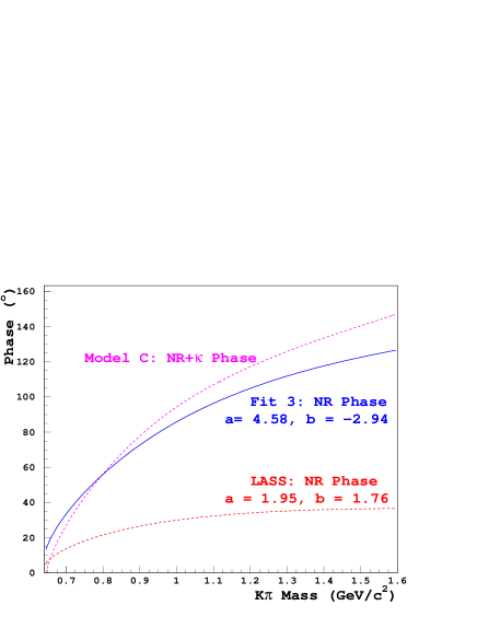
Figure 6: NR phase in Fit 3 compared to Model C and to LASS

A very interesting feature of Fit 3 is the negative value for $b$. In this case, the “effective-range” would be indicating a resonant behavior. To better show this effect, we plot in Fig.6 the $\delta_{B}$ phase motion of the “NR” decay in Fit 3 for the fitted values of $a$ and $b$. Note that the phase increases very rapidly from threshold. This effect is similar to the effect we found for $\kappa$. Here in Fit 3, the “effective-range” phase would be replacing that for a constant NR and the $\kappa$ in Model C (also shown in the figure); the two curves are very similar, even more if one realizes that one is mainly the result of a Breit-Wigner shape for the $\kappa$ and the other comes from what would be an effective-range form (but turned out to have an impressive phase variation). For comparison, the curve of $\delta_{B}$ with the parameters obtained by LASS are also shown: an almost constant phase for the NR was observed.

We see that the scalar sector at low $K\pi$ mass in $D^{+}\to K^{-}\pi^{+}\pi^{+}$ needs a rapidly-varying phase, consistent with the previous indication of the $\kappa$ state from dkpipi .

4 Conclusions

Using the Fermilab E791 data sample of $D^{+}\to K^{-}\pi^{+}\pi^{+}$ , we present new, preliminary studies offering further information concerning the phase motion behavior of the scalar amplitude at low $K\pi$ mass. In particular, we showed that the S-wave phase motion as measured by LASS in a scattering process is not able to describe the E791 decay data. This result shows the significance of final-state interactions in $D$ decays preventing a direct comparison of the phases in scattering and decay processes. Furthermore, an independent parametrization (without using a Breit-Wigner) provided a phase behavior consistent to what we found previously for the scalar low-mass $K\pi$ amplitude as a $\kappa$ meson.

References

- (1) E. M. Aitala et al. (E791 collaboration), Phys. Rev. Lett. 89, 121801 (2002).
- (2) E.M. Aitala et al. (E791 collaboration), Phys. Rev. Lett. 86, 770 (2001).
- (3) E.M. Aitala et al. (E791 collaboration), Phys. Rev. Lett. 86, 765 (2001).
- (4) D. Aston et al. (LASS Collaboration), Nucl. Phys. B296, 493 (1988).
- (5) S. Amato et al., Nucl. Instrum. Meth. A324, 535 (1993); S. Bracker and S. Hansen, hep-ex/0210034; S. Hansen et al., IEEE Trans. Nucl. Sci. 34, 1003 (1987)
- (6) J.C. Anjos et al. (E691 Collaboration) , Phys. Rev. D 48, 56 (1993).
- (7) P.L. Frabetti et al. (E687 Collaboration), Phys. Lett. B 331, 217 (1994).
- (8) W. Ochs, private communication.
- (9) J. M. Link et al. (FOCUS Collaboration), Phys. Lett. B 535 43, (2002).
- (10) W. Dunwoodie for the LASS Collaboration, private communication.