Limits on Production of Magnetic Monopoles Utilizing Samples from the DO and CDF Detectors at the Tevatron

Abstract

We present 90% confidence level limits on magnetic monopole production at the Fermilab Tevatron from three sets of samples obtained from the D0 and CDF detectors each exposed to a proton-antiproton luminosity of $\sim 175\mbox{ pb}^{-1}$ (experiment E-882). Limits are obtained for the production cross-sections and masses for low-mass accelerator-produced pointlike Dirac monopoles trapped and bound in material surrounding the D0 and CDF collision regions. In the absence of a complete quantum field theory of magnetic charge, we estimate these limits on the basis of a Drell-Yan model. These results (for magnetic charge values of 1, 2, 3, and 6 times the minimum Dirac charge) extend and improve previously published bounds.

I Introduction

The existence of even one magnetic monopole with magnetic charge $g$ explains the quantization of electric charge $e$ in terms of the Dirac quantization condition Dirac (1931) $eg=n\hbar c/2$, $n=\pm 1,\pm 2,\dots$. (Throughout this paper we use Gaussian units, but numerical results are expressed in SI.) Besides explaining the quantization of electric charge, the existence of magnetic charge results in the dual symmetrization of Maxwell’s equations Schwinger (1975a), and is not forbidden by any known principles of physics. The minimum magnitude of the quantization number is $n=1$ according to Dirac or $n=2$ according to Schwinger Schwinger (1975b). If $e$ is the charge of the electron, these magnitudes become $n=3,6$, respectively, if quantization via quark electric charges is possible. It should be emphasized that magnetic charge, like electric charge, is absolutely conserved, so the lightest magnetically charged particle is stable, unless annihilated by its antiparticle.

Throughout this paper we refer to magnetically charged particles as magnetic monopoles, or simply monopoles. However, as Schwinger emphasized Schwinger (1975a), magnetically charged particles could also carry electric charge; such particles he christened dyons. The quantization condition for a pair of dyons labeled 1 and 2 is

$$e_{1}g_{2}-e_{2}g_{1}=n\frac{\hbar c}{2}.$$ (1)

We will not explicitly mention dyons further. We merely note that the considerations here should supply similar cross section and mass limits on dyons as for monopoles. There would be modifications for dyons—for example, there would be a binding contribution due to electric Coulombic attraction or repulsion, but because electric charges are so much smaller that magnetic ones, the magnetic contributions are overwhelming. More significant probably are acceptance modifications, due to changes in energy loss, but we expect the quantitative impact of these changes to be small (less than 10%.)

If they exist, monopoles will presumably be abundant, or can be pair-produced by some appropriate mechanism, and be trapped in matter. Previous (direct) searches for trapped and bound magnetic monopoles in various accelerator samples Eberhard et al. (1975); Burke et al. (1975); Giacomelli et al. (1975); Carrigan et al. (1978); Aubert et al. (1983); Fryberger et al. (1984); Kinoshita et al. (1988, 1989); Pinfold et al. (1993); Bertani et al. (1990); Price et al. (1987, 1990), in meteorites Jeon and Longo (1995), and lunar soil Ross et al. (1973), as well as an earlier result Kalbfleisch et al. (2000); Luo (2002) from this experiment have been made. Other (indirect) searches by other methods are not covered in this paper, but are reviewed elsewhere Luo (2002); Giacomelli and Patrizii (2003). Here we report 1) a reanalysis of the data of Ref. Kalbfleisch et al. (2000), 2) the data of Luo Luo (2002) as well as 3) that of a third set of samples from the CDF detector recently measured and analyzed. This extension of limits is experimentally driven. Theoretical motivations derive from the expectation that monopoles from spontaneous electroweak scale symmetry breaking might give rise to monopoles of mass $\sim 2.5$ to $\sim 15$ TeV Preskill (1984); Kirkman and Zachos (1981), although we here can only search out to a mass, in our Drell-Yan modeling, $\sim 0.4$ TeV. The LHC using this method would allow one to approach 2 TeV. Unfortunately no accelerator is currently envisioned that will reach the theoretically interesting region of 10 to 15 TeV. In view of our nearly complete absence of knowledge of the origin of particle masses, we should not exclude any mass region from an experimental search.

This paper presents the experiment, analyses, and results of our search for monopoles. Section II outlines the basics of the detector apparatus; details are provided elsewhere Luo (2002). Section III covers the calibration and linearity of the detector. Section IV discusses the samples and monopole energy loss leading to the stopping and capture of monopoles in the sample material. Section V describes the analysis of the measurements. Section VI discusses the transformation of the data to monopole cross-sections and mass limits. Finally we summarize in Section VII.

II Magnetic Monopole Detector

We use the induction method of Alvarez, et al. Eberhard et al. (1971); Alvarez (1963) to detect monopoles. A large warm bore cryogenic detector, similar to that of Jeon and Longo Jeon and Longo (1995), was constructed at the University of Oklahoma. The active elements of the detector, shown schematically in Fig. 1,

Figure 1: Schematic radial cross-section of the monopole detector at a 2:1 width to height ratio. The elements generally are rings, tubes, or cylinders concentric with the indicated centerline. The height, which was 155 cm during the set 1 measurements of the D0 aluminum samples, was increased to 185 cm for the subsequent CDF lead and aluminum samples.

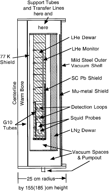
are two 19 cm diameter superconducting loops each connected to a dc SQUID (superconducting quantum interference device). The magnetic flux from a magnetic multipole passing through the loop induces a change in the loop’s supercurrent because the Meissner effect prevents a change in the magnetic flux through such a loop. If the multipole is dipole or higher, then the total net change when the sample traverses the loop starting and ending at large distances goes to zero, although locally supercurrents are present when the sample is in the neighborhood of the loop. But if a monopole passes through the loop, then a nonzero net change in the supercurrent occurs, giving a current “step” characteristic of a magnetic charge. This effect can be observed from even one monopole in a macroscopic sample due to the long range ($\sim 1/r^{2}$) nature of the associated magnetic field. The change in supercurrent is detected by the SQUID connected to the loop and converted to a voltage by the SQUID’s preamplifier and controller (see below).

Measurement of samples of a size less than 7.5 cm in diameter by 8.5 cm in length is made by repeatedly passing them through the 10 cm diameter warm bore centered on and perpendicular to the loops. A vertical excursion of 1.1 m around the position of the loops is typically made. In a central 65 cm region this allows for the magnetic effects of induced and permanent dipole moments of the sample to start and return to zero on each up and each down traversal taking some 25 s each. A net data rate of 10 Hz is recorded for each of the SQUIDs. Also recorded are the readings of an accelerometer, the vertical position of the sample recorded by an optical encoder, the number of increments taken by the stepper motor moving the sample, and the time. The data acquisition (DAQ) was performed with Apple Macintosh computers running under National Instruments LABVIEW programs lab .

Other magnetic and electronic signals affect the SQUIDs also, causing systematic errors. One has to deal with:

1. Permanent dipoles in the samples (presumably microscopic particles of magnetite or other ferrites)

2. Induced dipoles (because the samples are conducting metals)

3. Contamination of the transporting nylon string and copper wire

4. Ground loops

5. External electronic device interference (certain clocks, welding operations, etc.)

6. Thunderstorms (which forced suspension of operations)

7. Mechanical vibrations (external limited by dampers and isolation, internal due to cryogen boiling)

8. Small variations in the warm bore magnetic field gradient

9. Unidentified sources (some days operations had to be suspended).

In addition to data running, background running was required, which was subtracted from the data runs. Even during good running conditions, source (3) was always present to some degree. Source (1) was present for most samples; large dipole moments off-center in the volume of the sample give dipole tails that are unbalanced and can mimic monopole steps. Samples with large dipole signals need to be vetoed, because the SQUID loses count of the number of flux quanta. Induced signals, source (2), which are oppositely directed on up/down traversals, are pairwise cancelled. The temporal dependence of these signals [a complete sample measurement takes some twenty (20) minutes] is minimized by using only time-coincident traversals from the two squids taking data. It is to be noted that source (1) is variable. On repeat traversals, the magnitude of the dipole signal may change, most likely because the magnetite grains may be re-magnetized. The induced dipole signal, source (2), is proportional to the conductivity of the sample, the magnetic field gradient in the warm bore, and the velocity of the sample. The velocity used (one meter per 25 seconds) kept the magnitude smaller than the permanent dipole value in general.

Sporadic electrical and electronic interferences listed above occasionally caused automatic resets of the SQUID controllers. The operator had to restore the output levels of the SQUIDs manually and continue the measurement. Later, in the analysis stage, these reset (bad) data traces are vetoed pairwise.

III Calibration and Linearity

The schematic circuitry of the SQUIDs and the associated detection loops are shown in Fig. 2.

Figure 2: Schematic of the monopole detector’s signal measuring electronics. The flux passed through the superconducting loop, L1, is converted into a current change that induces a flux change in the DC SQUID ring. An induced feedback current is amplified and converted into the output signal voltage in the preamplifier/controller and processed by the LABVIEW data acquisition (DAQ) program running in the Macintosh computer.

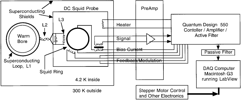
During operation of the experiment, the SQUIDs are tuned and their transfer functions measured periodically according to the manufacturer’s specifications to keep them operating with constant sensitivity. The sensitivity can be approximately predicted from the SQUID sensor’s parameters and accurately calibrated by measurement. The absolute calibration of an expected signal from a Dirac monopole is made using a “pseudopole.” A long thin magnetic solenoid carrying a small known current gives a calculable pseudopole (ps) at either end. The pseudopole can either be passed through the warm bore of the detector in a way similar to the samples (discussed later), or it can be placed in a given position with one end fully extended through the SQUID loops and the solenoid current repeatedly switched on and off. Both methods were used. We now discuss the parameters and the calibration.

The expected response function ($\mbox{RF}=\frac{dV}{d\Phi_{\rm loop}}$) of the SQUID system depends on the following parameters (where the current to voltage conversion is done by the SQUID controller’s amplifiers):

$$\mbox{RF}=\frac{dV}{d\Phi_{\rm squid}}\frac{d\Phi_{\rm squid}}{dI}\frac{dI}{d\Phi_{\rm loop}}\quad\mbox{in}\quad\mbox{V}/\phi_{0},$$ (2)

where $dI$ is the change in current induced in the SQUID sensor, $d\Phi_{\rm squid}$ is the flux change in the SQUID, $d\Phi_{\rm loop}$ is the flux change in the detection loop, $\phi_{0}$ is $hc/2e=2.07\times 10^{-15}$ Wb, the superconducting fluxoid unit, and $dV$ is the change in output voltage of the SQUID controller. Our SQUIDs were two junction DC types manufactured by Quantum Design C (1).

$dV/d\Phi_{\rm squid}$ is the so-called transfer function, “XF,” measured by a test pulse injection procedure given by the manufacturer, for our SQUIDs approximately 0.5–0.8 $V/\phi_{0}$. $d\Phi_{\rm squid}/dI$ is a parameter measured and furnished by the manufacturer. $dI/d\Phi_{\rm loop}$ is calculated as follows. Since the magnetic flux linking a superconducting loop is conserved as a result of the Meissner effect, we have by integrating the generalized Maxwell equation

$$-\bm{\nabla}\times\mathbf{E}=\frac{1}{c}\frac{d\mathbf{B}}{dt}+\frac{4\pi}{c}\mathbf{J}_{m},$$ (3)

$\mathbf{J}_{m}$ being the magnetic current density, the following relation for the current induced in the detection loop by one flux quantum passing through it (see Appendix):

$$I=\frac{\phi_{0}}{c}\frac{\left(1-\left(\frac{r}{a}\right)^{2}\right)}{L_{1}+L_{2}+L_{3}},$$ (4)

where (see Fig. 2) $L_{1}$ is the inductance of the detection loop, $L_{2}$ is the inductance of connecting twisted pair, $L_{3}$ is the input inductance of the squid sensor, $r$ is the radius of detection loop, and $a$ is the radius of the superconducting lead (Pb) shield. The factor $(1-(r/a)^{2})$ inserted in Eq. (4) corrects for the trapping of flux coupled into the detection loop due to the cylindrical superconducting shield. (See Appendix.)

The sensor’s input coil inductance $L_{3}$ is measured to be of order 1.8 $\mu$H (see Table 1). The inductance $L_{2}$ is zero, and $L_{1}$ (of order 1 $\mu$H) is calculated from the standard formula Schwinger et al. (1998); Stratton (1941):

$$L_{\rm loop}(C)=\frac{4\pi}{c^{2}}r\left(\ln\frac{8r}{\rho}-C\right),$$ (5)

where $r$ is the radius of the loop and $\rho$ is the wire radius. For a uniform current density in the loop $C=7/4$; for a (superconducting) surface current $C=2$ (a reduction in the inductance of 4 percent). In addition, the superconducting shield reduces the value of $L_{\rm loop}$ by 9.5 percent:

$$L_{1}=L_{\rm loop}(2)(1-0.095)=0.70\mu\mbox{H}.$$ (6)

This comes about as follows: The inductance between the detection loop and the superconducting shield is given by the following formula, rather easily derived from the inductance between two loops Stratton (1941):

$$L_{ls}=\frac{4\pi}{c^{2}}\int_{0}^{\pi}d\phi\,\sin^{2}\phi\frac{a^{2}r^{2}}{(a^{2}+r^{2}+2ar\cos\phi)(a^{2}+r^{2}+l^{2}+2ar\cos\phi)^{1/2}},$$ (7)

where $a$ is the radius of the shield and $2l$ its length. Inverting the inductance matrix changes the effective inductance of the detection loop by a significant amount

$$L_{1}=L_{\rm loop}\left(1-\frac{L_{ls}^{2}}{L_{\rm loop}L_{\rm shield}}\right),$$ (8)

and putting in the values $a=14.73$ cm, $r=9.855$ cm, $l=30$ cm, and $\rho=0.02$ cm gives $L_{1}$ as in Eq. (6), where $L_{\rm shield}=4\pi a^{2}/(2lc^{2})$ is the self-inductance of the superconducting cylindrical shield.

The experiment had four (4) SQUID sensors referred to as DC1, DC2, DC3, and DC4. DC1 failed at some early time, was repaired and subsequently called DC1R. Most of the sample measurements for the final analysis were performed with the pair DC1R and DC2. However, some measurements were made with other pairings of the four SQUIDs, and in a number of configurations, which are catalogued in the tables which follow. In initial tests, we had an emulation setup with a small bore and small detection loops immersed in liquid helium contained in a “Research Dewar.” We also had two current sources for the pseudopole, one having multiples of a current unit [$\sim 1.55$ V battery/500 M$\Omega$, equal to about 0.7 Dirac poles—see Eq. (10) below] equal to 1, 2, 5, 25, 100 current units and a later one with multiples of 1.7, 2.5, 5, 50 current units. We also had an early pseudopole of 0.5 meter length and a later one of 1.016 meter length. The actual currents for each number of units was measured with a picoammeter to be correlated with the voltage response of the calibration measurements.

The individual measured transfer functions, XF, in $V/\phi_{0}$ are given in Fig. 3.

Figure 3: The myriad of transfer function (XF $=dV/d\Phi_{\rm squid}$) measurements made over the course of the monopole experiment. Time intervals for the SQUID configurations in use at the various times, as well as the periods of measurement of the different sample sets are also indicated. RD $=$ research dewar, D0 and CDF are the collider experiments from which the samples were taken, RM $=$ remeasurements and 1, 2, 3, 4 refer to the various SQUID probes (see text).

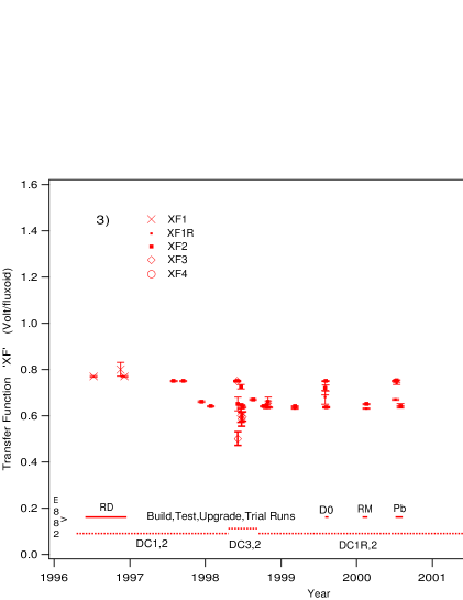
We see two lines of values at 0.75 and 0.64 for most of the plot, with values of 1.5 and 1.3 at year 2002.5, where we doubled the output gain of the squid controllers. The double valuedness is due to the presence or absence of an external passive RC low pass filter, which exhibits attenuation to the signal before being converted on the ADC board in the computer. (The controller has an internal active low pass filter which can be switched on or off, which in comparison is attenuation-free well below the rolloff point.) Table 1 identifies in the name DCi the filter configuration as “NF” or “EF” for “no filter” (or non-attenuating active internal filter) or “external filter,” respectively. In the table, *2 or RD indicate the doubled gain or early Research Dewar data. A gain 0.5 data point was taken while testing modifications to the controllers, and is exactly half of the gain 1.0 point above it (see Fig. 3). The transfer functions and their errors shown in Fig. 3 have been averaged as appropriate and entered into Table 1. Table 1 also shows the $d\Phi_{\rm squid}/dI$ values, the input coil inductances $L_{3}$, the $dI/d\Phi_{\rm loop}$ values calculated from Eq. (4), and the theoretical RF’s [Eq. (2)] shown (mV/Dirac pole). Note one Dirac pole corresponds to two fluxoid units, $4\pi g=hc/e$.

Table 1: Transfer functions and predictions. The subscript $s$ denotes SQUID. Here $\{L_{1},1-(r/a)^{2}\}=\{0.70\,\mu\mbox{H},0.552\}$ for all entries except for the first (RD) where they are $\{0.01\,\mu\mbox{H},0.87\}$. Remember $\phi_{D}=2\Phi_{0}$. $\Delta(dV/d\Phi_{s})$ is the error in $dV/d\Phi_{s}$, and likewise $\Delta({\rm RF}_{\rm th})$ is the error in ${\rm RF}_{\rm th}$.

Point	SQUID/Filter	$dV/d\Phi_{s}$	$\Delta(dV/d\Phi_{s})$	$d\Phi_{s}/dI$	$L_{3}$	$dI/d\Phi_{\rm loop}$	${\rm RF}_{\rm th}$	$\Delta({\rm RF}_{\rm th})$
		(V/$\phi_{0}$)		($\phi_{0}$/$\mu$A)	($\mu$H)	(nA/$\phi_{0}$)	(mV/$\phi_{D}$)
0	DC1NFRD	0.770	0.002	5.24	1.88	0.953	7.69	0.15
1	DC1NF	0.770	0.002	5.24	1.88	0.442	3.56	0.08
2	DC1RNF	0.739	0.005	5.24	1.85	0.447	3.46	0.08
3	DC1REF	0.637	0.004	5.24	1.85	0.447	2.98	0.07
4	DC2NF	0.752	0.001	4.17	1.47	0.525	3.29	0.09
5	DC2EF	0.643	0.002	4.17	1.47	0.525	2.82	0.07
6	DC3NF	0.750	0.003	5.24	1.85	0.447	3.51	0.08
7	DC3EF	0.643	0.015	5.24	1.85	0.447	3.01	0.10
8	DC4NF	0.741	0.001	3.94	1.43	0.535	3.12	0.08
9	DC4EF	0.633	0.003	3.94	1.43	0.535	2.67	0.07
10	DC1RNF*2	1.473	0.005	5.24	1.85	0.447	6.90	0.15
11	DC1REF*2	1.260	0.002	5.24	1.85	0.447	5.90	0.13
12	DC2NF*2	1.455	0.003	4.17	1.47	0.525	6.37	0.17
13	DC3NF*2	1.252	0.005	5.24	1.85	0.447	5.86	0.13
14	DC3EF*2	1.110	0.005	5.24	1.85	0.447	5.20	0.12

The experimental data (mV/nA) for traversals of the pseudopole through the warm bore, as with samples, and for the pseudopole “parked” at one position and its current turned on and off, are shown in Fig. 4a and 4b, respectively. The two methods agree within experimental uncertainties.

Figure 4: Individual measured pseudopole responses (mV/nA) for a) traversing the loop similarly as the samples and b) turning the current on/off while the pseudopole is “parked” at one position.

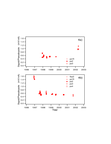
One again sees (at early times) the RD data, then the normal mid-year data, and finally the doubled gain data in 2002. Averaging the appropriate groupings of DCi gives the values (mV/nA) in Table 2.

Table 2: Measured pseudopole responses and comparisons to predictions (Table 1). (Note: mV/nA $\times$ nA/$\phi_{D}$ = mV/$\phi_{D}$.) Here “Ratio” is the ratio of the theoretical response RF_th given in Table 1 to the measured response/pole.

Point	SQUID/Filter	Response	$\Delta$(Response)	$i$/pole	Response/pole	$\Delta$(Response/pole)	Ratio
		(mV/nA)		(nA/$\phi_{D}$)	(mV/$\phi_{D}$)
0	DC1NFRD	1.44	0.02	4.40	6.34	0.10	1.21
1	DC1NF			4.63
2	DC1RNF			4.63
3	DC1REF	0.51	0.01	4.63	2.36	0.05	1.26
4	DC2NF	0.62	0.003	4.63	2.87	0.02	1.14
5	DC2EF	0.535	0.002	4.63	2.48	0.02	1.14
6	DC3NF			4.63
7	DC3EF	0.444	0.014	4.63	2.06	0.07	1.46
8	DC4NF			4.63
9	DC4EF	0.513	0.003	4.63	2.38	0.02	1.12
10	DC1RNF*2	1.15	0.01	4.63	5.32	0.06	1.30
11	DC1REF*2	0.97	0.013	4.63	4.49	0.07	1.31
12	DC2NF*2			4.63
13	DC3NF*2			4.63
14	DC3EF*2	0.97	0.016	4.63	4.50	0.08	1.15

The conversion from the response in mV/nA to that in mV/Dirac pole is given by considering the pseudopole solenoid’s magnetic moment both as a current loop and as a pole-antipole dipole, i.e.,

$$gL=\frac{1}{c}NiA$$ (9)

where the length of solenoid is $L=1.016\,(0.50)$ m for the new (old) pseudopole, respectively, $Ni$ is the ampere-turns of current, $N=4710\,(2440)$ turns, and the cross-sectional area of the solenoid is $A=1.533\pm 0.011\times 10^{-4}\,\mbox{m}^{2}$, so that (in SI, $g_{D}/\mu_{0}=3.29\times 10^{-9}$ A m)

$$\frac{i}{\rm pole}=\frac{gc}{(N/L)A}=4.63(4.40)\pm 0.03\,\mbox{nA}/\phi_{D},$$ (10)

for the new (old) pseudopole, respectively.

Using these conversion values we get the measured pseudopole response in mV/$\phi_{D}$ pseudopole values versus DCi configuration shown in Table 2 and Fig. 5a and the expected/measured ratio in Table 2 and Fig. 5b, respectively. A weighted average of these ratios for the nine values is $1.21\pm 0.07$. The discrepancy is presumably due to approximate values of Quantum Design’s measured parameters, and the elementary treatment excluding shielding internal to the SQUID probes, etc.

Figure 5: Experimental calibration of squid responses (a) as compared to predictions (b). The values from (a) are used in the data analysis of the samples below. The identity of the respective squid is indicated by “Point.”

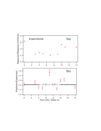
The values plotted in Fig. 5a are used to determine cuts on the possible monopole “steps” seen in the analysis of the data given later below. Data taken at year 1997.7 give the linearity response shown in Fig. 6a and 6b.

Figure 6: Linearity for no filter and for passive filter for a) the whole range of pseudopole currents and b) expanded. The units of current (about 0.7 Dirac pole, see text) are indicated. This is data from DC2 (1997) for the short pseudopole.

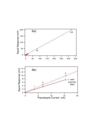
One sees that the calibration is very linear, and that signals down to one-half a Dirac pole can, in practice, be measured.

The shape of an expected monopole step is obtained by a subtraction of two runs with different pseudopole currents, as shown in Fig. 7a.

Figure 7: a) Pseudopole response, SQUID DC2, versus position for two currents, $\pm 50$ current units (about $\pm 35$ Dirac poles) and their difference, giving the experimental monopole step shape, and b) several such shapes [one of DC1R, three of DC2 including 7a) above, and one of DC3] compared, and c) Fig. 7a compared to the theoretically expected shapes: loop in free space (poor) Barger and Ollson (1967) and in a superconducting can (SC) (good)–see Appendix.

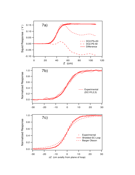
Five such shapes are compared in Fig. 7b. The theoretical modeling, given in the Appendix, is compared to the experimental data in Fig. 7c. The agreement between the theoretical and experimental shapes is good. We conclude that the calibration, linearity, and positional response (shape) indicate that the experiment is understood, and that operating conditions over six years are reasonably consistent and stable.

IV Samples, Stopping and Trapping

IV.1 Samples

There were three sets of samples obtained from discarded material from the upgrading of the D0 D0 Collaboration (1994) and CDF Bedeachi et al. (1988) detectors: 1) Be beam pipe and Al “extension” cylinders from D0, 2) Pb from the forward/backward “FEM” (Forward ElectroMagnetic calorimeters) of CDF, and 3) half of the Al cylinder (“CTC” support) from CDF. Sample set 1 was initially reported Kalbfleisch et al. (2000), 2 was given in Luo’s PhD. thesis Luo (2002), and set 3 here. In this paper, all three sets are being reported according to a final consistent analysis.

Sample set 1 comes from the two Al extension cylinders (extending beyond the main central detectors of D0 inside the liquid argon calorimetry), each of 150 cm diameter by 46 cm length by 1.26 cm thickness. They came as 16 plates. Four of these plates were further cut by water jet, whereas the balance were cut on a bandsaw; no magnetic degradation was observed from the bandsawing in comparison to the water jet samples. These cut pieces were 7 cm by 7.6 cm or 6 cm by 7.6 cm in size. Two of each were bundled into a “cylinder” constituting a “sample.” There are a total of 222 Al samples. The Al sawings and other small scrap pieces are accounted for later.

In addition, sample set 1 included the D0 5 cm diameter, 0.05 cm thickness Be beam pipe. The central 46 cm section, centered on the collision region and covering nearly the full solid angle, was cut into six 7.6 cm pieces.

Sample set 2 comes from twelve 2 m by 2 m by 0.5 cm thick Pb sections cut from the center of the full 3.04 m by 3.04 m Pb layers. These twelve layers were those closest to the interaction region of which six were located on the east side and the other six on the west. Each layer had an octagonal hole at the center (of approximately 30 cm “diameter”) for the passage of the $\overline{p}$-$p$ beams, etc. Each 2 m by 2 m section came as six pieces of 0.667 m by 1 m, labeled T (top), M (middle) or B (bottom) and also labeled N (north) or S (south). The six sections were also labeled as E (east) or W (west) and by layer number (1,2…,6). These sections were sheared into twelve strips of 8.3 cm width across the 1.00 m dimension, and each strip was rolled into a cylinder of approximately 7.5 cm diameter. These constitute some 816 samples. A typical layer is shown in Fig. 8.

Figure 8: A lead sample layer is cut into 68 samples. The Monte Carlo simulation shows that only the samples (52 in one layer) subtending an angle $3^{\circ}<\theta<7.5^{\circ}$ have significant acceptance and should be considered. The cross-hatched samples and others with cuts on large $dS$ (statistical) and $sS$ (systematic) errors are excluded from the analysis; the (solid angle) coverage falls to 53% for $n=1$ monopoles (see text).

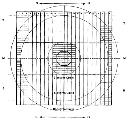
Of the 816 samples, only 664 have been successfully measured. The rest were unmeasurable due to huge dipole moments caused by the (ferromagnetic) red paint on the first layer samples. Fortunately, layer 1 samples turn out not to be needed. The large solenoidal magnetic field of CDF accelerates the monopoles to a high enough energy (70$n$ GeV additional) that they penetrate the early layers, reaching layers 4, 5, 6 for $n=1$ and layer 2 for $n=2,3$, and not at all for $n=6$. The scrap pieces and other unmeasurable samples of Pb are accounted for later.

Sample set 3 comes from the CDF’s inner support cylinder, which has eight 0.63 cm thick cover plates on a cylinder of 2.74 m diameter by 2.64 m length. Six of these cover plates, covering three-quarters of the azimuthal angle about the beam direction, were made into samples, similar to the D0 ones. These were sheared on a large shearing machine, first into long strips and then each strip into shorter sections. Eight pieces (four of each size) were bundled into a 7.5 cm diameter by 7.6 cm long cylinder (the CDF Al being half the thickness of the D0 extension pieces) yielding 404 samples with little scrap. Due to limitations on time, funding and personnel, 132 of the samples did not get measured, leading to only one-half the azimuthal solid angle being covered. These and the scrap are accounted for later below.

It turns out that all of the CDF Al samples were very magnetic (similarly to the CDF Pb red painted layer 1 samples). We had to demagnetize them. Degaussing with an AC field coil was ineffective. But as ferrites have Curie points below 585 ^∘C Kittel (1986) and the melting point of Al is 660 ^∘C (as opposed to 327 ^∘C for Pb), we were able to demagnetize all but a few of the samples by a heat treatment, “soaking” the samples at 610 ^∘C for one hour. The dipole amplitudes decreased from an unmanageable 3–10 V to the usual 30–100 mV.

IV.2 Stopping of the Monopoles

IV.2.1 Energy Loss

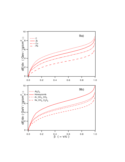
The energy losses ($dE/dx$) of magnetic monopoles traversing material absorbers are caused by the interaction of the moving monopole charge ($g=ng_{D}$) with the electric field of the atomic electrons, i.e., the $g{\bf v\times E}$ Lorentz force. The velocity dependence of this force cancels the 1/(velocity)² dependence of the usual charged particle $dE/dx$. Either classically Schwinger et al. (1998), quantum mechanically Schwinger et al. (1976), or field theoretically Gamberg and Milton (2000), approximately one simply substitutes $(g\beta)^{2}$ for $(ze)^{2}$ in the usual charged particle $dE/dx$ formula. Kazama, Yang, and Goldhaber Kazama et al. (1977) have obtained the differential scattering cross section for an electron moving in the magnetic field of a fixed magnetic pole. Ahlen Ahlen (1982, 1978) has used this cross-section to obtain the following expression for monopole stopping power:

$$-\frac{dE}{dx} = \frac{4\pi}{c^{2}}\frac{g^{2}e^{2}}{m_{e}}N_{e}\bigg{(}\ln\frac{2m_{e}c^{2}\beta^{2}\gamma^{2}}{I}+\frac{1}{2}K(|n|)$$ (11)

$$\quad\mbox{}-\frac{1}{2}\delta-\frac{1}{2}-B(|n|)\bigg{)},$$

where $N_{e}$ is the number density of electrons, $I$ is the mean ionization energy, $K(|n|)=0.406$ (0.346) is the Kazama, Yang and Goldhaber correction for magnetic charge $n=1$ ($n\geq 2$) respectively, $\delta$ is the usual density correction and $B(|n|)=0.248$ (0.672, 1.022, 1.685) is the Bloch correction for $n=1$ ($n=2,3,6$), respectively Hagiwara et al. (2002). (Of course, one must divide by the density to get $dx$ in g/cm².) This formula is good only for velocities $\beta=v/c\gtrsim 0.1$. For velocities $\beta\lesssim 0.01$, we use Eq. (60) of Ref. Ahlen and Kinoshita (1982) as an approximation for all materials:

$$-\frac{dE}{dx}=(45\mbox{ Gev/cm})n^{2}\beta,$$ (12)

which is linear in $\beta$ in this region. The two $dE/dx$ velocity regions are joined by an empirically fitted polynomial in the region of $\beta=0.01$–0.1 in order to have a smooth function of $\beta$. For the elemental and composite materials found in the D0 and CDF detectors, we show the resulting $dE/dx$ curves we used in Fig. 9. (See Ref. Luo (2002).)

Figure 9: $dE/dx$ vs $\beta$ ($=v/c$) for a) elements and b) compounds and mixtures involved in the energy losses of monopoles passing through the various detector materials. To increase legibility of the elemental figure, we have not shown the energy loss for Si and Be, which are similar to Al, nor for N₂, which is similar to C. For the compounds and mixtures, we note that C₃H₆, CO₂–C₂H₆–Al, and Rohacell are similar to Honeycomb, and SiO₂ is similar to Al₂O₃. These $dE/dx$ curves are for a magnetic charge value of $n=1$; apart from the correction terms $K(|n|)$ and $B(|n|)$, we multiply by $n^{2}$ for larger magnetic charge values.

IV.2.2 Stopping of Possible Monopoles

The trajectories of possible monopoles are generated in a Monte Carlo program from the collision point through the appropriate detector elements slowing to a stop in the sample layers, including the acceleration (or deceleration) of the monopole along the external magnetic field lines of the CDF detector. The average polar angle $\theta$ relative to the beam direction is different for the three sample sets: $\theta=35^{\circ}$, $6.5^{\circ}$, and $90^{\circ}$ for sets 1, 2, and 3, respectively. The amount of material along a “typical” trajectory is shown in Table 3 for D0 and Table 4 for CDF.

Table 3: The materials and path lengths at an angle of $35^{\circ}$ relative to the beam direction for the D0 aluminum sample measurements (set 1).

Detector	Material	Path lengths (g/cm2)
	Be pipe	0.16
VTX	C2H6 and CO2 gas, Al wire mixture	0.12
TRD	Al window	2.18
	N2 gas	0.01
	Polypropylene	1.12
	Xe, CH4, C2H6 gases	0.02
	Honeycomb	1.99
CDC	Ar, CO2, CH4 gases	0.07
	Kapton	0.1
	Rohacell	0.49
	Endplate (Al)	4.18
	G10	1.11
Total including	Sample layer (Al)	11.6–17.6

Table 4: The materials and path lengths in the CDF detector, at an angle of $6.5^{\circ}$ from the beam for CDF lead samples (set 2), and at an angle of $90^{\circ}$ from the beam for the CDF aluminum samples (set 3). The Pb samples are spaced by 0.6 g/cm² of drift chambers.

		Set 2	Set 3
Detector	Material	Path lengths (g/cm2) at $6.5^{\circ}$	Path lengths (g/cm2) at $90^{\circ}$
	Be pipe	0.82	0.092
SVX	C	—	0.209
	Al	—	0.135
	Si	—	0.210
	Al2O3	0.29	—
VTPC	C	3.57	0.312
FTC/CTC	Al	FTC:  0.25	CTC:  0.293
	Pb layer and drift chamber	6.5
Total including	Sample layers	Pb layer 2: 11.4–17.2	Al: 1.25–2.97
		Pb layer 4: 24.5–30.2
		Pb layer 5: 31.1–36.8
		Pb layer 6: 37.6–43.3

IV.2.3 Trapping of Monopoles

The monopoles having been stopped can then bind to the magnetic moments of the nuclei of the material present, and are therefore trapped. The interaction of the monopoles with the magnetic moments of nuclei and electrons can be strong enough to produce bound states under certain conditions and be trapped, having a very long lifetime in such bound states Gamberg et al. (2000). The trapping efficiency is very high. The theoretical modeling that has been done assumes “rigid” extended nuclei with or without repulsive barriers, and some relativistic calculations have also been carried out. Electrons can bind to monopoles in a total energy zero state; this probably produces a small mobile system which will transfer to a nuclear magnetic moment leaving it bound to a fixed nuclear site and permanently trapped. Thus we assume all monopoles bind to appropriate nuclei, i.e., those whose nuclear gyromagnetic ratio is sufficiently large (anomalous). These models predict, as summarized in Ref. Gamberg et al. (2000), that binding should occur for ²⁷Al (100% natural abundance) and ²⁰⁷Pb (22% natural) but not for ⁹Be (100% natural). However, the estimated binding energies, e.g., 0.5–2.5 MeV for aluminum, are large and comparable to shell model splittings, so we believe that in the presence of the monopole the nucleus will undergo nuclear rearrangement and binding should in general result, even for ⁹Be. Even an unreasonably small estimate for the binding energy of 1 eV would give a lifetime of 10 yr Gamberg et al. (2000). We have, therefore, good reason to believe that stopped monopoles will be trapped by the magnetic moments of nuclei.

V Analysis of the Data

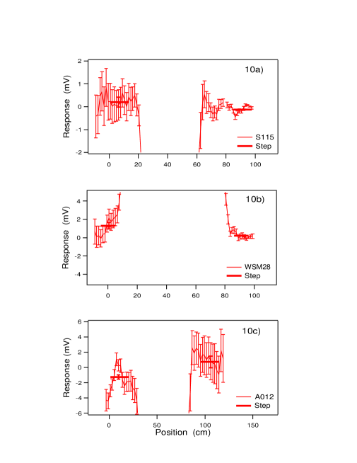
The data analysis proceeded generally as follows, with modifications as required for the different sets of samples. The time sequences of the SQUID’s outputs were examined interactively, and bad sections, primarily sections that contained a SQUID reset (see Sec. II), deleted pairwise (to keep induced signals canceling out pairwise) and the corresponding traces on the other SQUID also deleted (to keep them temporally consistent); typically 80–90% of the traversals remained. A pedestal value, the SQUID output near the top end of each traversal (bottom for sample set 3), was subtracted from every voltage value along that up (or down) traversal. The values for each of some 90 (75 for sample set 3) small ranges of vertical positions were averaged, removing most of the random drift of the SQUIDs. The two SQUIDs’ data were averaged, shifting one relative to the other by 10.1 cm in position in order to superimpose their dipole responses. The background samples were analyzed similarly and local groups of background runs were averaged. These background runs were subtracted from the samples’ spectra. A pair of horizontal lines was fit to two regions, one at the lower position and one at the upper. The difference in values of these two flat fits gives the step for that sample. Examples of processed data are shown, one for each sample set, in Fig. 10.

Figure 10: Typical step plots: a) set 1, D0 aluminum, sample “S115,” b) set 2, CDF lead, sample “WSM28,” and c) set 3, CDF aluminum, sample “A012.” The steps are $-0.4$, $-1.1$, and 2.0 mV, respectively.

The steps for each sample set are histogramed and analyzed for consistency with the null hypothesis, absence of monopoles. The background subtraction ensures that the distribution of steps centers on zero, since various background effects, such as the small effect of the magnetized string holding the sample in set 1, has been removed. These analyses were performed with a large set of macro procedures written for the program WaveMetrics’ IGOR-Pro igo running on Apple Macintosh computers.

For sample set 1 (D0 aluminum and beryllium) the background sequence was one background sample (always the same sample) between every two samples measured. For sample set 2 (CDF lead) it was one background between every three samples. And for sample set 3, the other samples were used as backgrounds for any given sample. The background averaging was done over time blocks of data. Each time the measurements were interrupted for unmanned time, a liquid helium fill, a thunderstorm, etc., some possible change in the environmental background was likely, so these were considered time blocks that required an independent background subtraction.

Sample set 2’s sample holder was a threaded metal rod with hexagonal nuts clamping the rolled lead sample cylinder. The overall magnetic dipole background was generally dominated by the sample holder, making the analysis of the CDF lead samples a bit harder than those of sample set 1.

Sample set 3 differed most in its procedures. A greater signal sensitivity should give a better overall signal-to-noise ratio for each SQUID’s data. As a major part of the noise was external to the SQUID electronics, the overall gain of the controllers was increased (see Section III above) by doubling feedback resistor values and halving capacitor values of the final operational amplifiers. This sensitivity gain apparently would have occurred. However, as the experiment was winding down, with time, funding and manpower coming to an end, the failure of one of the two SQUIDs for set 3 was not repaired (in consideration of the time that would have been lost to warm-up, repair, cool-down, etc.). The remaining SQUID had a small 0.4 Hz oscillation which we then dealt with in the analysis software, by smoothing the spectrum over a number of the 10 Hz data input values before editing the traversals. In addition, we extended the range of the traversals to 1.2 meter, at a larger stepper motor interval, leading to fewer (the 75 bins mentioned above) vertical position bins. The IGOR macros were modified to allow the computer to delete pairs of traces based on a chi-squared test of the consistency of differing traces in a sample’s traversals from the average of those minimally edited (for bad traces, resets, etc.). Chi-squareds per degree of freedom greater than two were rejected, corresponding to a ten percent loss of traces on average.

VI Monopole Cross-Sections and Mass Limits

The analyses of Sec. V above yield a number of “step” histograms. Those for set 1, D0 aluminum and beryllium, are shown in Fig. 11,

Figure 11: Histogram of the steps from 222 aluminum and 6 beryllium samples from the D0 experiment. The total of 228 samples, with an rms spread of 0.73 mV, is compared to a Gaussian with that same standard deviation.

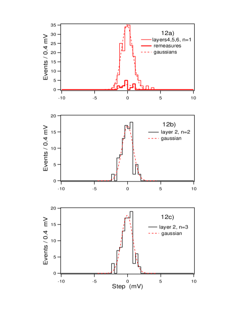
for set 2, CDF lead, in Fig. 12,

Figure 12: Histograms of the steps for the CDF lead samples, with an rms dispersion of 0.85 mV. a) 187 layer 4, 5, 6 samples along with the 14 remeasurements, having $sS<0.3$ mV and $dS<0.45$ mV, b) 90 layer 2 samples having $sS<0.4$ mV and $dS<0.6$ mV, and c) 95 layer 2 samples having $sS<0.6$ mV and $dS<0.8$ mV. Also shown are the four corresponding Gaussians for comparison. Note that the distributions in a), b), c) are used for limits on magnetic charges of $|n|=1,2,3$, respectively.

and for set 3, the CDF aluminum samples, in Fig. 13

Figure 13: Histogram of the steps from 240 aluminum samples ($sS<1.0$ mV) from the CDF experiment, with an rms dispersion of 2.7 mV (reflecting a higher gain setting of SQUID DC1R, see text) compared to the appropriate Gaussian. These data are used for limits for the three magnetic charge values $|n|=2,3$, and 6.

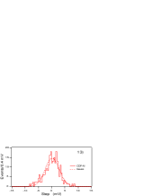
after taking account of the cuts on the errors discussed below.

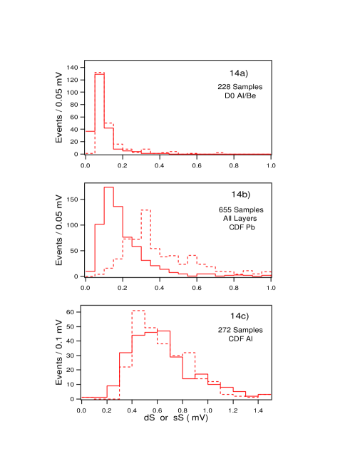
In these plots the variable $dS$ is the standard statistical error on the step $S$, whereas $sS$ is a systematic error which is the rms of the deviations of the actual step from the flat fitted steps shown, e.g., in Fig. 10. If the distribution is flat (with little slope) $sS$ is small, whereas if it is badly sloped it is large. Bad measurements, e.g., very large dipole tails, etc., cannot give a true measure of the step $S$, and so are removed by this cut. Note that Fig. 10b has a wide dipole response, but still an acceptable $sS$; its wide dipole response comes about because it is the superposition of two dipoles separated in position. Some cases cut by a large $sS$ are due to larger or more complicated superpositions of dipole responses. The histograms of $dS$ and $sS$ are shown in Fig. 14: cuts on $dS$ and $sS$ are made in order to control the dispersion of the step histograms, and losses of events are taken into account in the efficiency $\epsilon$ defined below.

Figure 14: The error histograms for $dS$ (dashed) and $sS$ (solid) for sample sets 1, 2 and 3 (remember the higher gain setting for set 3). Note that the the individual $(dS,sS)$ error values for the step plots a, b, c, shown in Figure 10, are (0.22, 0.08), (0.34, 0.32) and (0.82, 0.48) mV, respectively.

A number of parameters need to be taken from these plots and interpreted to yield the cross section and mass limits desired. Each plot determines an upper limit on the number ($N_{\rm ul}$) of monopoles of a given magnetic charge ($n=1,2,3,6$) for each sample set which in turn determines an upper limit to the corresponding cross-section

$$\sigma<\frac{N_{\rm ul}}{\varepsilon\epsilon A\mathcal{L}},$$ (13)

where $\varepsilon$ is the efficiency for the chosen signal (a monopole with charge $n$) to lie outside a cut excluding smaller values of $|n|$, $\epsilon$ is the efficiency of the sample set to cover the solid-angle region chosen and to correct for $dS$ and $sS$ cut losses, and to account for losses of sample material. $\mathcal{L}$ is the total luminosity for the $\overline{p}$-$p$ exposure delivered ($172\pm 8\mbox{pb}^{-1}$ for D0 Tartaglia and $180\mbox{pb}^{-1}$ $\pm 5$% for CDF lum (8 March 1996)).

The Drell-Yan modelling is that Kalbfleisch et al. (2000) $d\sigma/dM_{\rm pair}\sim(\beta/M_{\rm pair})^{3}$, where $\beta$ is the velocity of the monopole in the rest frame of the monopole-antimonopole pair. This basic cross section, involving the interaction suppression factor of $\beta^{2}$, is multiplied by the phase space $\beta$ and convolved with the CETQ5 Lai et al. (2000) quark-parton distributions (PDFs). In Ref. Kalbfleisch et al. (2000) we normalized the integral of this cross section to $(g/e)^{2}\sim 4700n^{2}$ times the experimental CDF and D0 $p\bar{p}\to\mu\bar{\mu}$ cross sections Abe et al. (1994); Abbott et al. (1999); Kalbfleisch et al. (2000) and obtained the $\sigma(M\bar{M})$ Drell-Yan cross section. For Luo’s thesis Luo (2002) an a priori theoretical normalization was made, by inserting the quark-antiquark to mu pairs cross section,

$$\sigma(q\bar{q})=\frac{4\pi\alpha^{2}e_{q}^{2}}{3Q^{2}},$$ (14)

where $e_{q}$ is the quark charge and $Q$ is the mass of the quark pair, in place of $d\sigma/dM$ above. The summing over quark charges and convolving with PDFs, etc., was also done. This procedure agrees with the first one within a factor of two, and is stable with respect to choice of PDF (e.g., MRST Martin et al. (1998)). Equation (14) has integrated out a $1+\cos^{2}\theta$ center-of-mass angular distribution appropriate to a $\mu\bar{\mu}$ virtual photon vertex. The Drell-Yan Monte Carlo puts this factor back into the equation and throws weighted events according to the mass and angular distributions of the model. The thrown monopole events are Lorentz transformed to the laboratory frame and tracked through the various structural materials into the appropriate sample(s). We also take into account the acceleration or deceleration due to any external magnetic fields present ($\sim 30n$ GeV/m for CDF). Those events entering and stopping in the sample layer(s) are summed into the “accepted” cross section $\sigma_{A}$. The acceptance is then $A=\sigma_{A}/\sigma$, where $\sigma$ is the total cross section without any path length or angle cuts.

In order to extract $N_{\rm ul}$, we must make cuts on the step histograms, as shown in Fig. 15.

Figure 15: A schematic of the upper limit number analysis parameters needed to obtain the cross-section limits via Tables 5 and 6.

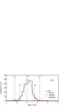
We define a region about zero using $C_{0}$ (i.e., $0\pm C_{0}$) such that most (zero) steps lie there, leaving most of the potential $n\neq 0$ charges lying outside of this region. The $C_{0}$ to $\infty$ and $-\infty$ to $-C_{0}$ region defines truncated Gaussians for magnetic charge $\pm n$, whose standard deviation is assumed (in the absence of further information) to be the same as that of the central (zero) peak, and shown as the small offset Gaussians in the figure. These are centered upon the expected positions of the charge $n$ monopoles, which is $n$ times the pseudopole calibration value from Table 2, Sec. III. Then $\varepsilon$ is the fractional area of these truncated Gaussians between $C_{0}$ and infinity. Also, the expected number ($N_{\rm exp}$) of null events outside $\pm C_{0}$ is the fraction of the central Gaussian lying outside times the total number of events in the histogram. This number is to be compared to the observed number ($N_{\rm obs}$) lying outside. We use the Feldman-Cousins tables of $N_{\rm exp}$ vs $N_{\rm obs}$ to find $N_{\rm ul}$ Feldman and Cousins (1998) at 90% confidence level. These parameters are compiled and displayed in Tables 5 and 6, from which $\sigma$ is calculated and tabulated (the lower limit on the monopole mass, $m_{\rm LL}$, is discussed below).

Table 5: Summary of parameters for the various sample sets and the various magnetic charge values ($n$) of the step histograms needed via Fig. 15. Here “response” refers to the mean value expected for a monopole of strength $n$. The table lists only those samples that have sufficient sensitivity for that value of $n$.

Set	$n$	Dispersion	$C_{0}$	Response	$N$	$N_{\rm exp}$	Nobs
		(mV)	(mV)	(mV)
1 Al	1	0.73	1.47	2.46	222	9.8	8
1 Al RM	1	0.73	1.47	2.46	8	0.4	0
2 Pb	1	0.85	1.6	2.46	187	11.2	14
2 Pb RM	1	0.85	1.6	2.36	14	0.8	0
1 Al	2	0.73	3.0	4.92	222	0	0
2 Pb	2	0.85	3.5	4.92	90	0	0
3 Al	2	2.7	8.8	10.64	240	0.3	0
1 Be	3	0.73	3.0	7.38	6	0	0
2 Pb	3	0.85	3.5	7.38	95	0	0
3 Al	3	2.7	8.8	16.0	240	0.3	0
1 Be	6	0.73	3.0	14.8	6	0	0
3 Al	6	2.7	8.8	31.9	240	0.3	0

Table 6: The remaining parameters and final limits (90% confidence level) from Drell-Yan modeling for cross-sections and monopole masses. The upper limit $N_{\rm ul}$ comes from a Feldman-Cousins analysis Feldman and Cousins (1998). Note: Set I Al RM and 2 Pb RM (lines 2 and 4) are corrected for losses of samples not remeasured by dividing by $\varepsilon$ again.

Set	$n$	$N_{\rm ul}$	$\varepsilon$	$\epsilon$	$A_{+1}$	$\mathcal{L}$	$\sigma^{\rm ul}_{+1}$	$m^{\rm LL}_{+1}$
		(90% CL)				(pb-1)	(pb)	(GeV/$c^{2}$)
1 Al	1	4.4	0.91	0.94	0.026	172	1.2	250
1 Al RM	1	2.0	0.91	0.94	0.026	172	0.6	275
2 Pb	1	10.3	0.84	0.53	0.013	180	9.9	180
2 Pb RM	1	1.7	0.82	0.53	0.011	180	2.4	225
1 Al	2	2.4	1.00	0.94	0.007	172	2.1	280
2 Pb	2	2.4	0.95	0.83	0.017	180	1.0	305
3 Al	2	2.1	0.75	0.88	0.10	180	0.2	365
1 Be	3	2.4	1.00	1.0	0.0036	172	3.9	285
2 Pb	3	2.4	1.00	0.87	0.028	180	0.5	350
3 Al	3	2.1	0.997	0.88	0.19	180	0.07	420
1 Be	6	2.4	1.00	1.0	0.013	172	1.1	330
3 Al	6	2.1	1.00	0.88	0.057	180	0.2	380

The only non-standard cases are the remeasurements of sets 1 and 2, in which the loss of possible monopole events not remeasured has to be taken into account, by another division by $\varepsilon$, as remarked in Table 6. We note that the cross-section limits range from 0.07 to 9.9 pb, a considerable improvement over earlier results from other experiments.

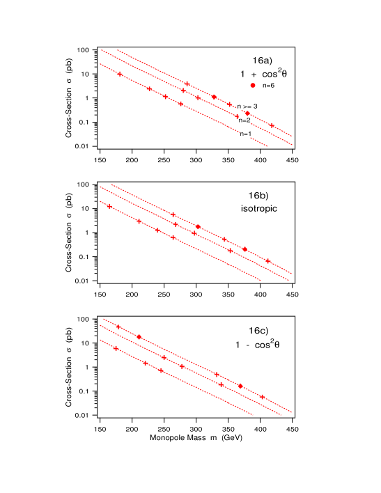
The above results are based on an model using a $1+\cos^{2}\theta$ angular distribution, appropriate for the coupling of spin-1/2 leptons to photons. As the angular distribution of magnetic monopoles is unknown, we try also two other distributions to give a flavor of the changes that would occur: isotropic (i.e., 1) and $\sin^{2}\theta=1-\cos^{2}\theta$. These alternative possibilities are given in Table 7. The total Drell-Yan cross-sections for these three angular distributions are in the ratio of 1 : 3/4 : 1/2 respectively when interpreting as mass limits.

Table 7: Alternative interpretations for different production angular distributions of the monopoles, comparing $1$ and $1-\cos^{2}\theta$ to the (repeated here) $1+\cos^{2}\theta$ limits. Here the acceptance $A_{a}$ corresponds to the distribution $1+a\cos^{2}\theta$, and similarly for the cross section and mass limits (all at 90% confidence level).

Set	$n$	$\sigma^{\rm ul}_{+1}$	$m^{\rm LL}_{+1}$	$A_{0}$	$\sigma^{\rm ul}_{0}$	$m^{\rm LL}_{0}$	$A_{-1}$	$\sigma^{\rm ul}_{-1}$	$m^{\rm LL}_{-1}$
		(pb)	(GeV/$c^{2}$)		(pb)	(GeV/$c^{2}$)		(pb)	(GeV/$c^{2}$)
1 Al	1	1.2	250	0.024	1.2	240	0.021	1.4	220
1 Al RM	1	0.6	275	0.024	0.6	265	0.021	0.7	245
2 Pb	1	9.9	180	0.011	12	165	0.0055	23	135
2 Pb RM	1	2.4	225	0.009	2.9	210	0.0045	5.9	175
1 Al	2	2.1	280	0.0068	2.2	270	0.0060	2.5	250
2 Pb	2	1.0	305	0.018	0.9	295	0.016	1.1	280
3 Al	2	0.2	365	0.10	0.2	355	0.096	0.2	340
1 Be	3	3.9	285	0.0025	5.6	265	0.0003	47	180
2 Pb	3	0.5	350	0.029	0.5	345	0.031	0.5	330
3 Al	3	0.07	420	0.20	0.07	410	0.24	0.06	405
1 Be	6	1.1	330	0.008	1.7	305	0.0008	18	210
3 Al	6	0.2	380	0.066	0.2	375	0.082	0.2	370

The cross-section limits above are model dependent, but only moderately so, since only the shape of the $d\sigma/dM_{\rm pair}$ distributions is relevant to the acceptance $A$, apart from the straightforward angular distribution, $dE/dx$, and magnetic field tracking considerations. The interpretation of these limits as monopole mass limits is directly model dependent. We have used the Drell-Yan model for lack of any field theoretic results. (For the status of the theory, see Ref. Gamberg and Milton (2000).) We modify the couplings from $e^{2}/\hbar c$ to $g^{2}/\hbar c$ (as appropriate in $dE/dx$ calculations) rather naively, but we have also included $\beta^{3}$ velocity suppression factors, a conservative choice. Moreover, we note that there is a unitarity limit that comes in at $n\approx 3$, and we use $n=3$ cross-sections as the unitarity limit for all $n\geq 3$ (i.e., we use three cross-sections, those for $n=1$ and $n=2$, and that for $n=3$ for higher $n$). Then, taking the intersection of the $\sigma$ limits with the Drell-Yan curves we obtain the lower limit for the mass (to the nearest 5 GeV) of each given monopole case, as entered in Tables 6 and 7, and shown in Fig. 16. These mass limits are an improvement of a factor of about two or more over previous direct experimental results.

Figure 16: The curves are Drell-Yan cross sections versus monopole mass with cross-section upper limits (90% CL) interpreted as mass limits (cross section upper limit intersects Drell-Yan curve at estimated lower limit of mass as shown by $+$ and $\bullet$ markers). Three possible center-of-mass angular distributions are considered, of form $1+a\cos^{2}\theta$, with $a=1$, 0 and $-1$, respectively.

VII Summary

We have improved the cross-section and mass limits on directly produced magnetic monopoles over the best previous other limits of Bertani et al. Bertani et al. (1990) and the lunar rock limits of Ross et al. Ross et al. (1973). We have improved and extended our own prior limits from D0 samples Kalbfleisch et al. (2000) to those from CDF, with a consistent overall analysis, presented in this paper.

Since limits are given, it is hard to assign errors. However, we can give a range or “spread” of the values from the quoted means to give a flavor of the variations to be expected. These spreads are in general a combination of statistical and systematic errors. Since we are modelling according to the Drell-Yan process, the systematic errors on the acceptances are unknown; it would take the evaluation of another reasonable proposed model, or a true quantum field theoretic prediction, to assess that. For example, a factor of two change in the cross section would lead to a change in the mass limits of about 20 GeV. The acceptances are estimates in any case, since the modeling of the detector elements, the $dE/dx$ losses, and the tracking of the particles through the various elements are not exact. The statistical error on the acceptances are 3% individually and 1% from smoothing over a mass interval (with a quadratic functional fit) of some 9–11 calculations spanning a 200–300 GeV mass region. The efficiencies ($\varepsilon$ and $\epsilon$) are good to about 2% and the luminosities to some 5%. Combining 3%, 2%, 2%, and 5% quadratically gives a spread of $\sim\pm 7$% on $\sigma_{\rm ul}$ in addition to the variations due to differing assumed angular distributions. Since the Dress-Yan cross sections are closely linear on a semilog plot against mass, this converts to a $\sim\pm 1$ GeV spread in mass. The unknown angular distributions give a greater uncertainty.

Since the true angular distributions are unknown, we take as a “base” an isotropic one (at 90% CL). In addition, we choose the largest mass limit for each value of the magnetic charge $n$. These come from D0 Al set 1 for $n=1$, and CDF Al set 3 for $n=2,3$ and 6. From Fig. 16 and Table 7, we see that these have cross section limits of 0.6, 0.2, 0.07, and 0.2 pb, respectively. The corresponding mass limits are 265, 355, 410, and 375 GeV, with spreads of ($+10,-20$), ($+10,-15$), ($+10,-5$), and $\pm 5$, respectively, due to replacing isotropic distributions by ones of the form $1\pm\cos^{2}\theta$.

These cross section limits are some 250 to 2500 times smaller and the mass limits are about 3 times larger than those of Bertani et al. Bertani et al. (1990), and a significant improvement over those of Ross et al. Ross et al. (1973), as well.

*

Appendix A Simplified Theory of Monopole Detector

This appendix describes the basis of the functioning of our magnetic monopole dectector. It works by detecting the magnetic flux intercepted by a superconducting loop contained within a superconducting cylinder. The detector is sketched in Fig. 17.

Figure 17: Diagram of monopole detector

In order to incorporate finite-size effects, we consider first a perfectly conducting right circular cylinder of radius $a$ of semi-infinite length, with axis along the $z$-axis, and with a perfectly conducting circular bottom cap at $z=0$. We use cylindrical coordinates $\rho$, $\theta$, and $z$.

Because the boundaries are superconductors, the normal component of $\bf B$ must vanish on the surfaces, that is,

$$B_{\rho}\bigg{|}_{{\rho=a}\atop{z>0}}=0,\quad B_{z}\bigg{|}_{z=0}=0.$$ (15)

Now suppose a magnetic pole of strength $g$ is placed on the $z$ axis at $z=z^{\prime}>0$. This could either be a magnetic monopole (magnetic charge) or one pole of a very long electromagnet (“pseudopole”). Imagine a circular conducting loop of radius $r<a$ centered on the axis of the cylinder and perpendicular to that axis, with center at $z=Z$. Inside the cylinder and outside of the loop $\bf B$ is derivable from a magnetic scalar potential,

$${\bf B}=-\mbox{\boldmath{$\nabla$}}\phi_{M},$$ (16)

since we may ignore the displacement current, because the time variation is negligible. $\phi_{M}$ satisfies Poisson’s equation, in cylindrical coordinates:

$$\mbox{\boldmath{$\nabla$}}\cdot\mathbf{B} = -\left(\frac{1}{\rho}\frac{\partial}{\partial\rho}\rho\frac{\partial}{\partial\rho}+\frac{1}{\rho^{2}}\frac{\partial^{2}}{\partial\theta^{2}}+\frac{\partial^{2}}{\partial z^{2}}\right)\phi_{M}$$ (17)

$$= 4\pi g\delta({\bf r-r^{\prime}}),$$

where $\mathbf{r}^{\prime}$ is the position of the monopole, $\mathbf{r^{\prime}}=(\rho^{\prime},\theta^{\prime},z^{\prime})$. This is the equation for a Green’s function, which we can express in separated variables form. That is, we write

$$\phi_{M} = \frac{2}{\pi}\int_{0}^{\infty}dk\cos kz\cos kz^{\prime}$$ (18)

$$\quad\times\sum_{m=-\infty}^{\infty}\frac{1}{2\pi}e^{im(\theta-\theta^{\prime})}g_{m}(\rho,\rho^{\prime};k),$$

where, in view of the first boundary condition in Eq. (15), we may express the reduced Green’s function in terms of modified Bessel functions:

$$g_{m}(\rho,\rho^{\prime};k) = -4\pi gI_{m}(k\rho_{<})$$

$$\quad\times\left[K_{m}(k\rho_{>})-I_{m}(k\rho_{>})\frac{K^{\prime}_{m}(ka)}{I^{\prime}_{m}(ka)}\right],$$

where $\rho_{<}$ ($\rho_{>}$) is the lesser (greater) of $\rho$, $\rho^{\prime}$. If the monopole is confined to the $z$ axis, only the $m=0$ term survives:

$$\phi_{M} = -\frac{4g}{\pi}\int_{0}^{\infty}dk\cos kz\cos kz^{\prime}$$ (20)

$$\quad\times\left[K_{0}(k\rho)+I_{0}(k\rho)\frac{K_{1}(ka)}{I_{1}(ka)}\right],$$

which uses

$$I_{0}^{\prime}(x)=I_{1}(x),\quad K_{0}^{\prime}(x)=-K_{1}(x).$$ (21)

By integrating over the cross section of the loop using

$$\int_{0}^{x}dt\,t\,K_{0}(t) = -x\,K_{1}(x)+1,$$ (22a)

$$\int_{0}^{x}dt\,t\,I_{0}(t) = x\,I_{1}(x),$$ (22b)

we obtain the following formula for the magnetic flux subtended by the loop,

$$\Phi=\int d{\bf S\cdot B}=4\pi g\left[\eta(Z-z^{\prime})-F(Z,z^{\prime})\right],$$ (23)

where the step function is

$$\eta(x)=\left\{\begin{array}[]{cc}1,&x>0,\\ 0,&x<0,\end{array}\right.$$ (24)

and the response function is

$$F(z,z^{\prime}) = \frac{2}{\pi}\frac{r}{a}\int_{0}^{\infty}dx\,\sin x\frac{z}{a}\cos x\frac{z^{\prime}}{a}$$

$$\times\left\{K_{1}(xr/a)-I_{1}(xr/a)\frac{K_{1}(x)}{I_{1}(x)}\right\},$$

Now suppose that the pole is slowly moved from a point far above the loop, $z^{\prime}=+\infty$, to a point below the loop, $z^{\prime}=z_{0}$, $Z>z_{0}$. Then from Maxwell’s equation

$$\mbox{\boldmath{$\nabla$}}\times{\bf E}=-\frac{1}{c}\frac{\partial}{\partial t}{\bf B}-\frac{4\pi}{c}{\bf J}_{m},$$ (26)

where $\mathbf{J}_{m}$ is the magnetic current density, the emf induced in the loop is

$${\cal E}=\oint{\bf E}\cdot d{\bf l},=-\frac{d\Phi}{cdt}+\frac{4\pi}{c}g\delta(t),$$ (27)

if $t=0$ is the time at which the pole passes through the plane of the loop. The net change in emf gives rise to a persistent current $I$ in the superconducting loop,

$$LI=\int_{-\infty}^{\infty}{\cal E}dt=-\frac{1}{c}\Delta\Phi+\frac{4\pi}{c}g=\frac{4\pi}{c}gF(Z,z_{0}),$$ (28)

where $L$ is the inductance of the loop, and the response function $F$ is given in Eq. (LABEL:a11a). This is just a statement of the Meissner effect, that the flux change caused by the moving monopole is cancelled by that due to the current set up in the loop.

Now suppose that the loop is very far from the bottom cap, $Z\gg a$. Then only small $x$ contributes to the integral in Eq. (LABEL:a11a), and it is easy to see that

$$\int_{-\infty}^{\infty}{\cal E}dt=\frac{4\pi g}{c}\left(1-\frac{r^{2}}{a^{2}}\right),$$ (29)

so the signal is maximized by making the loop as small as possible, relative to the radius of the cylinder. We get the full flux of the monopole only for a loop in empty space, $a/r\to\infty$. This perhaps counterintuitive effect is due to the fact that the superconducting walls confine the magnetic flux to the interior of the cylinder. Thus for the superconducting can, the induced current in the detection loop caused by the passage of a monopole from $z^{\prime}=\infty$ to $z^{\prime}=0$ is

$$LI=\frac{4\pi g}{c}-\frac{\Delta\Phi}{c}=\frac{4\pi g}{c}-\frac{\Phi(z^{\prime}=0)}{c},$$ (30)

which yields the result (29) if one assumes that the magnetic field is uniform across the can’s cross section at the position of the loop when the pole is at the bottom, because all the flux must pass up through the can. If we consider, instead, an infinite, open-ended, superconducting cylinder, with the monopole passing from $z=+\infty$ to $z=-\infty$, at either extreme half the flux must cross the plane of the loop, so with the uniformity assumption we get the same result:

$$LI=\frac{4\pi g}{c}-\frac{\Delta\Phi}{c}=\frac{4\pi g}{c}\left(1-\frac{r^{2}}{a^{2}}\right).$$ (31)

The simple assumption of a uniform magnetic field is apparently justified by the exact result (29).

We conclude this appendix by noting how the exact calculation is modified for an infinite superconducting cylinder. In the magnetic scalar potential, the integral over $k$ mode functions in Eq. (18) is replaced by

$$\int_{-\infty}^{\infty}\frac{dk}{2\pi}e^{ik(z-z^{\prime})},$$ (32)

which has the effect of replacing the flux expression (23) by

$$\Phi=2\pi g[\epsilon(z-z^{\prime})-F(Z-z^{\prime},0)],$$ (33)

where

$$\epsilon(x)=\left\{\begin{array}[]{cc}1,&x>0,\\ -1,&x<0.\end{array}\right.$$ (34)

Then the induced current in the detection loop when the monopole passes from a point above the loop $z^{\prime}=Z+\xi$ to a point, equidistant, below the loop, $z^{\prime}=Z-\xi$, is

$$LI=\frac{4\pi g}{c}F(\xi,0)\to\frac{4\pi g}{c}\left(1-\frac{r^{2}}{a^{2}}\right),$$ (35)

where the last limit applies if $\xi/a\gg 1$. This result coincides with that in Eq. (29). The function $R(\xi)=\frac{1}{2}F(\xi,0)/(1-r^{2}/a^{2})+\frac{1}{2}$, corresponding to a monopole starting from a point $z_{1}$ far above the loop, $z_{1}-Z\gg a$, and ending at a point $z_{0}=Z-\xi$, is plotted as a function of $\xi$ for our parameter values in Fig. 7c, where it is shown to agree well with experimental data. This response function coincides with the result obtained from Eq. (28), because

$$F(Z,Z-\xi) = \frac{1}{2}F(2Z-\xi,0)+\frac{1}{2}F(\xi,0)$$ (36)

$$\approx \frac{1}{2}\left(1-\frac{r^{2}}{a^{2}}\right)+\frac{1}{2}F(\xi,0),$$

if $Z/a\gg 1$. This shows that the effect of the endcap (which of course is not present in actual detector) is negligible, demonstrating that the fact that the superconducting shield is of finite length is of no significance.

References

- Dirac (1931) P. A. M. Dirac, Proc. Roy. Soc. Lond. A133, 60 (1931).
- Schwinger (1975a) J. S. Schwinger, Science 188, 1300 (1975a).
- Schwinger (1975b) J. S. Schwinger, Phys. Rev. D12, 3105 (1975b).
- Eberhard et al. (1975) P. H. Eberhard, R. R. Ross, J. D. Taylor, L. W. Alvarez, and H. Oberlack, Phys. Rev. D11, 3099 (1975).
- Burke et al. (1975) D. L. Burke, H. R. Gustafson, L. W. Jones, and M. J. Longo, Phys. Lett. B60, 113 (1975).
- Giacomelli et al. (1975) G. Giacomelli et al., Nuovo Cim. A28, 21 (1975).
- Carrigan et al. (1978) J. Carrigan, Richard A., B. P. Strauss, and G. Giacomelli, Phys. Rev. D17, 1754 (1978).
- Aubert et al. (1983) B. Aubert, P. Musset, M. Price, and J. P. Vialle, Phys. Lett. B120, 465 (1983).
- Fryberger et al. (1984) D. Fryberger, T. E. Coan, K. Kinoshita, and P. B. Price, Phys. Rev. D29, 1524 (1984).
- Kinoshita et al. (1988) K. Kinoshita, M. Fujii, K. Nakajima, P. B. Price, and S. Tasaka, Phys. Rev. Lett. 60, 1610 (1988).
- Kinoshita et al. (1989) K. Kinoshita, M. Fujii, K. Nakajima, P. B. Price, and S. Tasaka, Phys. Lett. B228, 543 (1989).
- Pinfold et al. (1993) J. L. Pinfold et al., Phys. Lett. B316, 407 (1993).
- Bertani et al. (1990) M. Bertani et al., Europhys. Lett. 12, 613 (1990).
- Price et al. (1987) P. B. Price, G.-X. Ren, and K. Kinoshita, Phys. Rev. Lett. 59, 2523 (1987).
- Price et al. (1990) P. B. Price, G.-R. Jing, and K. Kinoshita, Phys. Rev. Lett. 65, 149 (1990).
- Jeon and Longo (1995) H. Jeon and M. J. Longo, Phys. Rev. Lett. 75, 1443 (1995), eprint hep-ex/9508003.
- Ross et al. (1973) R. R. Ross, P. H. Eberhard, L. W. Alvarez, and R. D. Watt, Phys. Rev. D8, 698 (1973).
- Kalbfleisch et al. (2000) G. R. Kalbfleisch et al., Phys. Rev. Lett. 85, 5292 (2000), eprint hep-ex/0005005.
- Luo (2002) W. Luo, Ph.D. thesis, University of Oklahoma (2002), UMI-30-56946 (AAT 3056946).
- Giacomelli and Patrizii (2003) G. Giacomelli and L. Patrizii (2003), hep-ex/0302011.
- Preskill (1984) J. Preskill, Ann. Rev. Nucl. Part. Sci. 34, 461 (1984).
- Kirkman and Zachos (1981) T. W. Kirkman and C. K. Zachos, Phys. Rev. D24, 999 (1981).
- Eberhard et al. (1971) P. H. Eberhard, R. R. Ross, L. W. Alvarez, and R. D. Watt, Phys. Rev. D4, 3260 (1971).
- Alvarez (1963) L. W. Alvarez (1963), UCRL-AGM-470.
- (25) http://www.ni.com/labview/.
- C (1) Quantum Design, 11578 Sorrento Valley Road, San Diego, CA 92121.
- Schwinger et al. (1998) J. Schwinger, L. L. DeRaad, Jr., K. A. Milton, and W.-y. Tsai, Classical Electrodynamics (Perseus Books/Westview Press, 1998).
- Stratton (1941) J. A. Stratton, Electromagnetic Theory (McGraw-Hill, 1941).
- Barger and Ollson (1967) V. Barger and M. G. Ollson, Classical Electricity and Magnetism (Allyn and Bacon, Boston, 1967).
- D0 Collaboration (1994) D0 Collaboration, Nucl. Instrum. Methods A338, 185 (1994).
- Bedeachi et al. (1988) F. Bedeachi et al., Nucl. Instrum. Methods A268, 50 (1988).
- Kittel (1986) C. Kittel, Introduction to Solid State Physics (John Wiley and Sons, New York, 1986), 6th ed., Table 2, p. 429.
- Gamberg et al. (2000) L. Gamberg, G. R. Kalbfleisch, and K. A. Milton, Found. Phys. 30, 543 (2000), eprint hep-ph/9906526.
- Schwinger et al. (1976) J. Schwinger, K. A. Milton, W.-y. Tsai, L. L. DeRaad, Jr., and D. C. Clark, Ann. Phys. 101, 451 (1976).
- Gamberg and Milton (2000) L. P. Gamberg and K. A. Milton, Phys. Rev. D61, 075013 (2000), eprint hep-ph/9910526.
- Kazama et al. (1977) Y. Kazama, C. N. Yang, and A. S. Goldhaber, Phys. Rev. D15, 2287 (1977).
- Ahlen (1982) S. P. Ahlen, pp. 259–290 (1982), in Wingspread 1982, Proceedings, Magnetic Monopoles.
- Ahlen (1978) S. P. Ahlen, Phys. Rev. D17, 229 (1978).
- Hagiwara et al. (2002) K. Hagiwara et al. (Particle Data Group), Phys. Rev. D66, 010001 (2002), p. 195.
- Ahlen and Kinoshita (1982) S. P. Ahlen and K. Kinoshita, Phys. Rev. D26, 2347 (1982).
- (41) http://www.wavemetrics.com/.
- (42) M. Tartaglia, private communication.
- lum (8 March 1996) Fermi News 19 (8 March 1996).
- Lai et al. (2000) H. L. Lai et al. (CTEQ), Eur. Phys. J. C12, 375 (2000), eprint hep-ph/9903282.
- Abe et al. (1994) F. Abe et al. (CDF), Phys. Rev. D49, 1 (1994).
- Abbott et al. (1999) B. Abbott et al. (D0), Phys. Rev. Lett. 82, 4769 (1999), eprint hep-ex/9812010.
- Martin et al. (1998) A. D. Martin, R. G. Roberts, W. J. Stirling, and R. S. Thorne, Eur. Phys. J. C4, 463 (1998), eprint hep-ph/9803445.
- Feldman and Cousins (1998) G. J. Feldman and R. D. Cousins, Phys. Rev. D57, 3873 (1998).