EUROPEAN ORGANIZATION FOR NUCLEAR RESEARCH

CERN-EP/2003-021

30 April 2003

Search for pair-produced

leptoquarks in e⁺e^- interactions

at $\sqrt{s}~{}\simeq~{}$189 – 209 GeV

The OPAL Collaboration

Abstract

A search for pair-produced leptoquarks is performed using $\mbox{e}^{+}\mbox{e}^{-}$ collision events collected by the OPAL detector at LEP at centre-of-mass energies between 189 and 209 GeV. The data sample corresponds to a total integrated luminosity of 596 pb^-1. The leptoquarks are assumed to be produced via couplings to the photon and the Z⁰. For a given search channel only leptoquark decays involving a single lepton generation are considered. No evidence for leptoquark pair production is observed. Lower limits on masses for scalar and vector leptoquarks are calculated. The results improve most of the LEP limits derived from previous searches for the pair production process by 10–25 GeV, depending on the leptoquark quantum numbers.

(Submitted to European Physical Journal C)

G. Abbiendi², C. Ainsley⁵, P.F. Åkesson³, G. Alexander²², J. Allison¹⁶, P. Amaral⁹, G. Anagnostou¹, K.J. Anderson⁹, S. Arcelli², S. Asai²³, D. Axen²⁷, G. Azuelos^18,a, I. Bailey²⁶, E. Barberio^8,p, R.J. Barlow¹⁶, R.J. Batley⁵, P. Bechtle²⁵, T. Behnke²⁵, K.W. Bell²⁰, P.J. Bell¹, G. Bella²², A. Bellerive⁶, G. Benelli⁴, S. Bethke³², O. Biebel³¹, O. Boeriu¹⁰, P. Bock¹¹, M. Boutemeur³¹, S. Braibant⁸, L. Brigliadori², R.M. Brown²⁰, K. Buesser²⁵, H.J. Burckhart⁸, S. Campana⁴, R.K. Carnegie⁶, B. Caron²⁸, A.A. Carter¹³, J.R. Carter⁵, C.Y. Chang¹⁷, D.G. Charlton¹, A. Csilling²⁹, M. Cuffiani², S. Dado²¹, A. De Roeck⁸, E.A. De Wolf^8,s, K. Desch²⁵, B. Dienes³⁰, M. Donkers⁶, J. Dubbert³¹, E. Duchovni²⁴, G. Duckeck³¹, I.P. Duerdoth¹⁶, E. Etzion²², F. Fabbri², L. Feld¹⁰, P. Ferrari⁸, F. Fiedler³¹, I. Fleck¹⁰, M. Ford⁵, A. Frey⁸, A. Fürtjes⁸, P. Gagnon¹², J.W. Gary⁴, G. Gaycken²⁵, C. Geich-Gimbel³, G. Giacomelli², P. Giacomelli², M. Giunta⁴, J. Goldberg²¹, E. Gross²⁴, J. Grunhaus²², M. Gruwé⁸, P.O. Günther³, A. Gupta⁹, C. Hajdu²⁹, M. Hamann²⁵, G.G. Hanson⁴, K. Harder²⁵, A. Harel²¹, M. Harin-Dirac⁴, M. Hauschild⁸, C.M. Hawkes¹, R. Hawkings⁸, R.J. Hemingway⁶, C. Hensel²⁵, G. Herten¹⁰, R.D. Heuer²⁵, J.C. Hill⁵, K. Hoffman⁹, D. Horváth^29,c, P. Igo-Kemenes¹¹, K. Ishii²³, H. Jeremie¹⁸, P. Jovanovic¹, T.R. Junk⁶, N. Kanaya²⁶, J. Kanzaki^23,u, G. Karapetian¹⁸, D. Karlen²⁶, K. Kawagoe²³, T. Kawamoto²³, R.K. Keeler²⁶, R.G. Kellogg¹⁷, B.W. Kennedy²⁰, D.H. Kim¹⁹, K. Klein^11,t, A. Klier²⁴, S. Kluth³², T. Kobayashi²³, M. Kobel³, S. Komamiya²³, L. Kormos²⁶, T. Krämer²⁵, P. Krieger^6,l, J. von Krogh¹¹, K. Kruger⁸, T. Kuhl²⁵, M. Kupper²⁴, G.D. Lafferty¹⁶, H. Landsman²¹, D. Lanske¹⁴, J.G. Layter⁴, A. Leins³¹, D. Lellouch²⁴, J. Letts^o, L. Levinson²⁴, J. Lillich¹⁰, S.L. Lloyd¹³, F.K. Loebinger¹⁶, J. Lu^27,w, J. Ludwig¹⁰, A. Macpherson^28,i, W. Mader³, S. Marcellini², A.J. Martin¹³, G. Masetti², T. Mashimo²³, P. Mättig^m, W.J. McDonald²⁸, J. McKenna²⁷, T.J. McMahon¹, R.A. McPherson²⁶, F. Meijers⁸, W. Menges²⁵, F.S. Merritt⁹, H. Mes^6,a, A. Michelini², S. Mihara²³, G. Mikenberg²⁴, D.J. Miller¹⁵, S. Moed²¹, W. Mohr¹⁰, T. Mori²³, A. Mutter¹⁰, K. Nagai¹³, I. Nakamura^23,V, H. Nanjo²³, H.A. Neal³³, R. Nisius³², S.W. O’Neale¹, A. Oh⁸, A. Okpara¹¹, M.J. Oreglia⁹, S. Orito^23,∗, C. Pahl³², G. Pásztor^4,g, J.R. Pater¹⁶, G.N. Patrick²⁰, J.E. Pilcher⁹, J. Pinfold²⁸, D.E. Plane⁸, B. Poli², J. Polok⁸, O. Pooth¹⁴, M. Przybycień^8,n, A. Quadt³, K. Rabbertz^8,r, C. Rembser⁸, P. Renkel²⁴, J.M. Roney²⁶, S. Rosati³, Y. Rozen²¹, K. Runge¹⁰, K. Sachs⁶, T. Saeki²³, E.K.G. Sarkisyan^8,j, A.D. Schaile³¹, O. Schaile³¹, P. Scharff-Hansen⁸, J. Schieck³², T. Schörner-Sadenius⁸, M. Schröder⁸, M. Schumacher³, C. Schwick⁸, W.G. Scott²⁰, R. Seuster^14,f, T.G. Shears^8,h, B.C. Shen⁴, P. Sherwood¹⁵, G. Siroli², A. Skuja¹⁷, A.M. Smith⁸, R. Sobie²⁶, S. Söldner-Rembold^16,d, F. Spano⁹, A. Stahl³, K. Stephens¹⁶, D. Strom¹⁹, R. Ströhmer³¹, S. Tarem²¹, M. Tasevsky⁸, R.J. Taylor¹⁵, R. Teuscher⁹, M.A. Thomson⁵, E. Torrence¹⁹, D. Toya²³, P. Tran⁴, I. Trigger⁸, Z. Trócsányi^30,e, E. Tsur²², M.F. Turner-Watson¹, I. Ueda²³, B. Ujvári^30,e, C.F. Vollmer³¹, P. Vannerem¹⁰, R. Vértesi³⁰, M. Verzocchi¹⁷, H. Voss^8,q, J. Vossebeld^8,h, D. Waller⁶, C.P. Ward⁵, D.R. Ward⁵, P.M. Watkins¹, A.T. Watson¹, N.K. Watson¹, P.S. Wells⁸, T. Wengler⁸, N. Wermes³, D. Wetterling¹¹ G.W. Wilson^16,k, J.A. Wilson¹, G. Wolf²⁴, T.R. Wyatt¹⁶, S. Yamashita²³, D. Zer-Zion⁴, L. Zivkovic²⁴

¹School of Physics and Astronomy, University of Birmingham, Birmingham B15 2TT, UK
²Dipartimento di Fisica dell’ Università di Bologna and INFN, I-40126 Bologna, Italy
³Physikalisches Institut, Universität Bonn, D-53115 Bonn, Germany
⁴Department of Physics, University of California, Riverside CA 92521, USA
⁵Cavendish Laboratory, Cambridge CB3 0HE, UK
⁶Ottawa-Carleton Institute for Physics, Department of Physics, Carleton University, Ottawa, Ontario K1S 5B6, Canada
⁸CERN, European Organisation for Nuclear Research, CH-1211 Geneva 23, Switzerland
⁹Enrico Fermi Institute and Department of Physics, University of Chicago, Chicago IL 60637, USA
¹⁰Fakultät für Physik, Albert-Ludwigs-Universität Freiburg, D-79104 Freiburg, Germany
¹¹Physikalisches Institut, Universität Heidelberg, D-69120 Heidelberg, Germany
¹²Indiana University, Department of Physics, Bloomington IN 47405, USA
¹³Queen Mary and Westfield College, University of London, London E1 4NS, UK
¹⁴Technische Hochschule Aachen, III Physikalisches Institut, Sommerfeldstrasse 26-28, D-52056 Aachen, Germany
¹⁵University College London, London WC1E 6BT, UK
¹⁶Department of Physics, Schuster Laboratory, The University, Manchester M13 9PL, UK
¹⁷Department of Physics, University of Maryland, College Park, MD 20742, USA
¹⁸Laboratoire de Physique Nucléaire, Université de Montréal, Montréal, Québec H3C 3J7, Canada
¹⁹University of Oregon, Department of Physics, Eugene OR 97403, USA
²⁰CLRC Rutherford Appleton Laboratory, Chilton, Didcot, Oxfordshire OX11 0QX, UK
²¹Department of Physics, Technion-Israel Institute of Technology, Haifa 32000, Israel
²²Department of Physics and Astronomy, Tel Aviv University, Tel Aviv 69978, Israel
²³International Centre for Elementary Particle Physics and Department of Physics, University of Tokyo, Tokyo 113-0033, and Kobe University, Kobe 657-8501, Japan
²⁴Particle Physics Department, Weizmann Institute of Science, Rehovot 76100, Israel
²⁵Universität Hamburg/DESY, Institut für Experimentalphysik, Notkestrasse 85, D-22607 Hamburg, Germany
²⁶University of Victoria, Department of Physics, P O Box 3055, Victoria BC V8W 3P6, Canada
²⁷University of British Columbia, Department of Physics, Vancouver BC V6T 1Z1, Canada
²⁸University of Alberta, Department of Physics, Edmonton AB T6G 2J1, Canada
²⁹Research Institute for Particle and Nuclear Physics, H-1525 Budapest, P O Box 49, Hungary
³⁰Institute of Nuclear Research, H-4001 Debrecen, P O Box 51, Hungary
³¹Ludwig-Maximilians-Universität München, Sektion Physik, Am Coulombwall 1, D-85748 Garching, Germany
³²Max-Planck-Institute für Physik, Föhringer Ring 6, D-80805 München, Germany
³³Yale University, Department of Physics, New Haven, CT 06520, USA

^a and at TRIUMF, Vancouver, Canada V6T 2A3
^c and Institute of Nuclear Research, Debrecen, Hungary
^d and Heisenberg Fellow
^e and Department of Experimental Physics, Lajos Kossuth University, Debrecen, Hungary
^f and MPI München
^g and Research Institute for Particle and Nuclear Physics, Budapest, Hungary
^h now at University of Liverpool, Dept of Physics, Liverpool L69 3BX, U.K.
ⁱ and CERN, EP Div, 1211 Geneva 23
^j and Manchester University
^k now at University of Kansas, Dept of Physics and Astronomy, Lawrence, KS 66045, U.S.A.
^l now at University of Toronto, Dept of Physics, Toronto, Canada
^m current address Bergische Universität, Wuppertal, Germany
ⁿ now at University of Mining and Metallurgy, Cracow, Poland
^o now at University of California, San Diego, U.S.A.
^p now at Physics Dept Southern Methodist University, Dallas, TX 75275, U.S.A.
^q now at IPHE Université de Lausanne, CH-1015 Lausanne, Switzerland
^r now at IEKP Universität Karlsruhe, Germany
^s now at Universitaire Instelling Antwerpen, Physics Department, B-2610 Antwerpen, Belgium
^t now at RWTH Aachen, Germany
^u and High Energy Accelerator Research Organisation (KEK), Tsukuba, Ibaraki, Japan
^v now at University of Pennsylvania, Philadelphia, Pennsylvania, USA
^w now at TRIUMF, Vancouver, Canada
^∗ Deceased

1 Introduction

In the Standard Model (SM) quarks and leptons appear as formally independent components. However, they show an apparent symmetry in terms of the family and multiplet structure of the electroweak interactions. Some theories beyond the SM [1] therefore predict the existence of new bosonic fields, called leptoquarks (LQ), mediating interactions between quarks and leptons. The interactions of leptoquarks with the known particles are usually described by an effective Lagrangian that satisfies the requirement of baryon and lepton number conservation and respects the SU(3)${}_{\mathrm{C}}~{}\otimes$ SU(2)${}_{\mathrm{L}}~{}\otimes$ U(1)_Y symmetry of the SM [2, 3]. This results in nine scalar ($S$) and nine vector ($V$) leptoquarks which are colour triplets or antitriplets and are grouped into weak isospin triplets ($S_{1}$ and $V_{1}$), doublets ($S_{1/2}$, $\tilde{S}_{1/2}$, $V_{1/2}$ and $\tilde{V}_{1/2}$) and singlets ($S_{0}$, $\tilde{S}_{0}$, $V_{0}$ and $\tilde{V}_{0}$). Their properties are shown in Tables 1 and 2. A charge eigenstate within a multiplet will be referred to as a “state” and denoted by $S_{I}(Q_{{\rm em}})$ or $V_{I}(Q_{{\rm em}})$, where $Q_{{\rm em}}$ is the electric charge in units of $e$.

LQ

$F$

$I_{3}$

$Q_{{\rm em}}$

decay

coupling

$\beta$

$e^{-}_{L}u_{L}$

$\lambda_{LS_{0}}$

$S_{0}$

2

0

$-1/3$

$e^{-}_{R}u_{R}$

$\lambda_{RS_{0}}$

$\frac{\lambda_{LS_{0}}^{2}+\lambda_{RS_{0}}^{2}}{2\lambda_{LS_{0}}^{2}+\lambda_{RS_{0}}^{2}}$

$\nu_{e}d_{L}$

$-\lambda_{LS_{0}}$

$\tilde{S}_{0}$

2

0

$-4/3$

$e^{-}_{R}d_{R}$

$\lambda_{R\tilde{S}_{0}}$

1

1

2/3

$\nu_{e}u_{L}$

$\sqrt{2}\lambda_{LS_{1}}$

0

$S_{1}$

0

0

$-1/3$

$\left\{\begin{array}[]{r}\nu_{e}d_{L}\\ e^{-}_{L}u_{L}\end{array}\right.$

$\begin{array}[]{r}-\lambda_{LS_{1}}\\ -\lambda_{LS_{1}}\end{array}$

1/2

$-1$

$-4/3$

$e^{-}_{L}d_{L}$

$-\sqrt{2}\lambda_{LS_{1}}$

1

$1/2$

$-2/3$

$\left\{\begin{array}[]{r}\nu_{e}\overline{u}_{L}\\ e^{-}_{R}\overline{d}_{R}\end{array}\right.$

$\begin{array}[]{r}\lambda_{LS_{1/2}}\\ -\lambda_{RS_{1/2}}\end{array}$

$\frac{\lambda_{RS_{1/2}}^{2}}{\lambda_{LS_{1/2}}^{2}+\lambda_{RS_{1/2}}^{2}}$

$S_{1/2}$

0

$-1/2$

$-5/3$

$\left\{\begin{array}[]{r}e^{-}_{L}\overline{u}_{L}\\ e^{-}_{R}\overline{u}_{R}\end{array}\right.$

$\begin{array}[]{r}\lambda_{LS_{1/2}}\\ \lambda_{RS_{1/2}}\end{array}$

1

$1/2$

$1/3$

$\nu_{e}\overline{d}_{L}$

$\lambda_{L\tilde{S}_{1/2}}$

0

$\tilde{S}_{1/2}$

0

$-1/2$

$-2/3$

$e^{-}_{L}\overline{d}_{L}$

$\lambda_{L\tilde{S}_{1/2}}$

1

Table 1: Quantum numbers and couplings for scalar leptoquarks. $F=3B+L$ is the fermion number which is a function of the baryon and lepton numbers $B$ and $L$, $Q_{{\rm em}}$ is the electric charge in units of $e$, $I_{3}$ is the third component of the weak isospin and $\beta$ is the branching ratio of the decay to a charged lepton and a quark of any flavour. Under the assumption of non-zero couplings only within a single generation of leptons, $u$ and $d$ denote up- and down-type quarks respectively, and the same Table applies to second and third generation leptoquarks with the obvious substitutions $e\rightarrow\mu,\tau$. In the last column, $\lambda^{2}$ is a shorthand for $\sum_{j}(\lambda^{ij})^{2}$, where $i$ denotes the lepton generation and j the quark flavour.

LQ

$F$

$I_{3}$

$Q_{{\rm em}}$

decay

coupling

$\beta$

$e^{-}_{L}\overline{d}_{R}$

$\lambda_{LV_{0}}$

$V_{0}$

0

0

$-2/3$

$e^{-}_{R}\overline{d}_{L}$

$\lambda_{RV_{0}}$

$\frac{\lambda_{LV_{0}}^{2}+\lambda_{RV_{0}}^{2}}{2\lambda_{LV_{0}}^{2}+\lambda_{RV_{0}}^{2}}$

$\nu_{e}\overline{u}_{R}$

$\lambda_{LV_{0}}$

$\tilde{V}_{0}$

0

0

$-5/3$

$e^{-}_{R}\overline{u}_{L}$

$\lambda_{R\tilde{V}_{0}}$

1

1

1/3

$\nu_{e}\overline{d}_{R}$

$\sqrt{2}\lambda_{LV_{1}}$

0

$V_{1}$

0

0

$-2/3$

$\left\{\begin{array}[]{r}\nu_{e}\overline{u}_{R}\\ e^{-}_{L}\overline{d}_{R}\end{array}\right.$

$\begin{array}[]{r}\lambda_{LV_{1}}\\ -\lambda_{LV_{1}}\end{array}$

1/2

$-1$

$-5/3$

$e^{-}_{L}\overline{u}_{R}$

$\sqrt{2}\lambda_{LV_{1}}$

1

$1/2$

$-1/3$

$\left\{\begin{array}[]{r}\nu_{e}d_{R}\\ e^{-}_{R}u_{L}\end{array}\right.$

$\begin{array}[]{r}\lambda_{LV_{1/2}}\\ \lambda_{RV_{1/2}}\end{array}$

$\frac{\lambda_{RV_{1/2}}^{2}}{\lambda_{LV_{1/2}}^{2}+\lambda_{RV_{1/2}}^{2}}$

$V_{1/2}$

2

$-1/2$

$-4/3$

$\left\{\begin{array}[]{r}e^{-}_{L}d_{R}\\ e^{-}_{R}d_{L}\end{array}\right.$

$\begin{array}[]{r}\lambda_{LV_{1/2}}\\ \lambda_{RV_{1/2}}\end{array}$

1

$1/2$

$2/3$

$\nu_{e}u_{R}$

$\lambda_{L\tilde{V}_{1/2}}$

0

$\tilde{V}_{1/2}$

2

$-1/2$

$-1/3$

$e^{-}_{L}u_{R}$

$\lambda_{L\tilde{V}_{1/2}}$

1

Table 2: Same as Table 1, but for vector leptoquarks.

Under these assumptions, only the masses and the couplings to right-handed and left-handed leptons, denoted by $\lambda_{\mathrm{R}}$ and $\lambda_{\mathrm{L}}$, remain free parameters, since the couplings to the electroweak gauge bosons are completely determined by the electric charge and the third component of the weak isospin, while the interactions with gluons are given by the colour charge. Each coupling can carry generation indices for the two fermions [3], so that $\lambda^{ij}$ couples a leptoquark to an $i^{th}$ generation lepton and a $j^{th}$ generation quark. In this note only leptoquark decays involving a single family of leptons are searched for, while no distinction is made between quarks from different generations. This corresponds to the simplifying assumption that $\lambda^{ij}\cdot\lambda^{mn}=0$ if $i\neq m$. The states with couplings both to right-handed charged leptons and left-handed neutrinos have an unknown branching ratio into a charged lepton and a quark, $\beta$, depending on the relative values of the couplings, while for all the other states $\beta$ has a known fixed value. Some leptoquarks with couplings to left-handed leptons have the same properties as scalar quarks in supersymmetric models with R-parity violation [4]. This is the case for $S_{0}(-1/3)$, $\tilde{S}_{1/2}(1/3)$ and $\tilde{S}_{1/2}(-2/3)$. The results obtained in this analysis can therefore also be interpreted in terms of these models.

Several experimental results constrain theories that predict the existence of leptoquarks. Searches for events with leptoquark single production, where a first generation leptoquark could be formed as a resonance between an electron and a quark, were performed by the ZEUS and H1 experiments at the ep collider HERA [5] and by the DELPHI and OPAL experiments at LEP [6]. Leptoquark masses, M_LQ, of $\mathcal{O}(100$ GeV) are excluded for $\lambda$ values greater than ${\cal O}(10^{-2})$. All LEP and Tevatron experiments have searched for events with leptoquark pair production [7, 8, 9], setting limits on M_LQ as a function of the branching ratio for decay into a charged lepton and a quark. The values of these limits range from 99 GeV to 275 GeV depending on the decay channel and the spin of the leptoquarks.

In this paper a search is presented for pair-produced scalar and vector leptoquarks of all three generations performed with the OPAL detector. Compared to single production by electron-quark interactions, pair production has the advantage that all states can be produced, including leptoquarks that decay only into a neutrino and a quark. Searches for this channel at LEP are able to explore the region of large decay branching ratio into quark-neutrino final states, where the Fermilab experiments have reduced sensitivity. The study is based on data recorded during the LEP runs from 1998 to 2000 at centre-of-mass energies, $\sqrt{s}$, between 189 and 209 GeV. The different values of $\sqrt{s}$ and the corresponding integrated luminosities are listed in Table 3.

In principle, leptoquarks of all three generations can be pair-produced in e⁺e^- collisions at LEP, by s-channel $\gamma$ or Z⁰ exchange and, in the case of first generation leptoquarks, by the exchange of a quark in the t- or u-channel [10]. The current upper limits on the couplings $\lambda$ to fermions are $\mathcal{O}(10^{-2})$ in the mass range kinematically accessible; this makes the t- or u-channel contribution to the first generation production cross-section (including interference between this channel and the $s$-channel) less than 1$\%$ of the pure $s$-channel contribution. Therefore, in the present analysis, only $s$-channel leptoquark production is considered. Consequently, for a given state the cross-section depends on the mass, the electric charge and the third component of the weak isospin, but is independent of the $\lambda$ couplings. On the other hand, for couplings smaller than ${\cal O}(10^{-6})$ the lifetime of leptoquarks would be sufficiently long to have interactions with the material of detector and to produce a secondary decay vertex, clearly separated from the interaction region of the electron beams. This topology is not considered here as the tracks of charged particles are required to come from the primary interaction vertex so that, to summarize, the present analysis covers the region $10^{-6}<\lambda<10^{-2}$.

The decay of a heavy leptoquark into a charged lepton and a quark leads to final states characterized by an isolated energetic charged lepton and a hadronic jet, while for decays into a quark and a neutrino, the final state would have large missing energy and a jet. Given the assumptions about the $\lambda$ couplings, the following topologies are considered for events resulting from the decay of a leptoquark-antileptoquark pair:
Class A: Two hadronic jets and two neutrinos; it consists of the final states $\nu_{l}\overline{\nu_{l}}u^{j}\overline{u}$^k and $\nu_{l}\overline{\nu_{l}}d^{j}\overline{d}$^k, where $l={\rm e},\mu,\tau$ and $u^{j}$, $d^{j}$ are up- and down-type quarks of the $j^{th}$ generation.
Class B: Two hadronic jets, one neutrino and one charged lepton of the same generation ($\nu_{l}l^{\pm}u^{j}d^{k}$).
Class C: Two hadronic jets and one pair of oppositely charged leptons of the same generation (${l^{+}l^{-}}u^{j}\overline{u}$^k, ${l^{+}l^{-}}d^{j}\overline{d}$^k).

YEAR	$\langle~{}\sqrt{s}~{}\rangle$  (GeV)	${\displaystyle\int}{\cal L}~{}dt$   (pb-1)
1998	188.6	169.1
1999	191.6	28.9
	195.5	72.3
	199.5	74.7
	201.7	39.2
2000	203.8	8.5
	205.1	69.6
	206.3	63.1
	206.6	63.8
	208.0	6.7
TOTAL		595.9

Table 3: Average centre-of-mass energies and corresponding integrated luminosities for the data samples used in the analysis. The search for vector leptoquarks includes only the data with $\sqrt{s}>195$ GeV.

2 The OPAL Detector

The OPAL detector is described in detail in [11]. It was a multi-purpose apparatus having nearly complete solid angle coverage. The central detector consisted of a system of tracking chambers inside a 0.435 T solenoidal magnetic field as well as of two layers of silicon microstrip detectors [12] surrounding the beam-pipe. The tracking chambers included a high-precision drift chamber, a large-volume jet chamber and a set of z-chambers measuring the track coordinates along the beam direction. The resolution on the transverse momentum of a track was given by $\sigma_{p_{t}}/p_{t}\simeq\sqrt{(0.02)^{2}+(0.0015\cdot p_{t})^{2}/({\rm GeV})^{2}}$ and the average angular resolution was about 0.3 mrad in $\phi$ and 1 mrad in $\theta$. A lead-glass electromagnetic calorimeter was located outside the magnet coil and covered the full azimuthal range for polar angles in the range of $\mid\cos(\theta)\mid<0.984$. It was divided into two regions: the barrel ($\mid\cos(\theta)\mid<0.82$) and the endcaps ($|\cos(\theta)|>~{}0.81$). The energy resolution for high momentum electrons was around 3%. The magnet return yoke, divided into barrel and endcap sections along with pole tips, was instrumented for hadron calorimetry in the region $\mid\cos(\theta)\mid<0.99$. Four layers of muon chambers covered the outside of the hadron calorimeter. Close to the beam axis the forward calorimeter and gamma catcher, together with the silicon-tungsten luminometer [13] and the forward scintillating tile counter [14], completed the geometrical acceptance down to 33 mrad from the beam direction.

3 Monte Carlo simulations

At lowest order the $s$-channel contribution to the differential cross section for the production of a pair of scalar leptoquarks of mass M_LQ in $\rm{e^{+}e^{-}}$ collisions at a centre-of-mass energy $\sqrt{s}$ is given by [10]

$$\frac{d\sigma_{S}}{d\cos{\theta}}~{}=~{}\frac{3\pi\alpha^{2}}{8s}\left(1~{}-~{}4\mathrm{M}_{\mathrm{LQ}}^{2}/s\right)^{\frac{3}{2}}\sin^{2}\theta\sum_{a=L,R}|k_{a}(s)|^{2}~{},$$ (1)

while for vector leptoquarks one has

$$\frac{d\sigma_{V}}{d\cos{\theta}}~{}=~{}\frac{3\pi\alpha^{2}}{8s}\left(1~{}-~{}4\mathrm{M}_{\mathrm{LQ}}^{2}/s\right)^{\frac{3}{2}}\left\{\frac{4+\left[1~{}-~{}3\left(1-4\mathrm{M}_{\mathrm{LQ}}^{2}/s\right)\right]\sin^{2}\theta}{1-\left(1~{}-~{}4\mathrm{M}_{\mathrm{LQ}}^{2}/s\right)}\right\}\sum_{a=L,R}|k_{a}(s)|^{2}~{},$$ (2)

where $\alpha$ is the electromagnetic coupling and

$$k_{a}(s)~{}=~{}-Q_{{\rm em}}~{}+~{}Q_{a}^{{\rm Z}}({\mathrm{e}})\frac{s}{s~{}-~{}{\rm M}_{{\rm Z}}^{2}~{}+~{}i{\rm M}_{{\rm Z}}\Gamma_{{\rm Z}}}Q^{{\rm Z}}({\mathrm{LQ}}).$$ (3)

Here $Q_{{\rm em}}$ is the electric charge of the leptoquark, ${\mathrm{M}}_{{\rm Z}}$ and $\Gamma_{{\rm Z}}$ are the mass and the width of the ${\rm Z}^{0}$ boson, and the couplings are given by

$$Q^{{\rm Z}}(\mathrm{LQ}) = \frac{I_{3}~{}-~{}Q_{{\rm em}}\sin^{2}\theta_{W}}{\cos{\theta_{W}}\sin{\theta_{W}}}~{},$$

$$Q^{{\rm Z}}_{L}(\mathrm{e}) = \frac{-\frac{1}{2}~{}+~{}\sin^{2}\theta_{W}}{\cos{\theta_{W}}\sin{\theta_{W}}}~{},$$ (4)

$$Q^{{\rm Z}}_{R}(\mathrm{e}) = \tan{\theta_{W}}~{},$$

with $I_{3}$ being the third component of the leptoquark weak isospin and $\theta_{W}$ the Weinberg angle.

The Monte Carlo generator LQ2 [15] is used to simulate leptoquark pair events. Initial state QED radiation is included. In LQ2 scalar leptoquarks decay isotropically in their rest frame, while the angular distribution of decay products of vector leptoquarks depends on the helicity state. The hadronization of the final state quark pair is performed by JETSET [16]. For scalar leptoquarks, samples of at least 1000 signal events are generated for each value of the leptoquark mass from M${}_{\mathrm{LQ}}=50$ GeV to the kinematic limit in steps of 10 GeV or less for all the different decay topologies at the centre-of-mass energies with the highest integrated luminosities (189, 196, 200 and 206 GeV). The search for vector leptoquarks includes only data with $\sqrt{s}>195$ GeV and the signal was simulated for M${}_{\mathrm{LQ}}\geq 70$ GeV. Since leptoquarks carry colour, they may hadronize before decaying if their couplings to fermions are small. This effect is evaluated from Monte Carlo samples of pair-produced scalar quarks decaying via R-parity violating couplings. These events have features similar to events of class C and allow the impact of this effect on the detection efficiencies and on the leptoquark mass reconstruction to be estimated and taken into account as a systematic uncertainty.

All relevant SM background processes are studied using various samples of simulated Monte Carlo events for each centre-of-mass energy in the data. Two-fermion events (Z^0∗/$\gamma^{\ast}$ $\rightarrow$ ff̄($\gamma$), with f = q,$\tau$ and denoted by 2f), are simulated with KK2f [17]. The Monte Carlo programs HERWIG [18], PHOJET [19], and BDK [20] are used to generate two-photon ($\gamma\gamma$) events with hadronic and leptonic final states. Other processes with four fermions in the final state, 4$\rm{f}$, including W^± and Z⁰ pair production, are simulated with grc4f [21] and KORALW [22]. JETSET [16] is used as the principal model for the hadronization. Besides the main samples alternative generators or hadronization models such as KORALZ [23], Vermaseren [24] and HERWIG [18], are used to check the expectation from the SM background. Generally, at each centre-of-mass energy, the number of simulated events for the background processes corresponds to at least fifteen times the integrated luminosity of the data, except for the $\gamma\gamma$ process where, at some centre-of-mass energies, Monte Carlo events corresponding to only about three times the data integrated luminosity are available.

The full response of the OPAL detector [25] is simulated for all the Monte Carlo events.

4 Analysis

All the leptoquark event topologies (classes A to C as defined in Section 1) are characterized by large charged track multiplicities and large number of energy deposits (clusters) in the calorimeters due to the hadronization of the quark pair. Moreover, in events of classes B and C, energetic and well-isolated charged leptons are present.

The tracks of charged particles reconstructed in the tracking system and the clusters in the electromagnetic and hadronic calorimeters are required to satisfy the same quality criteria as in [8]. To avoid double counting, calculations of quantities such as visible energy and transverse momentum are performed from charged particle tracks and from clusters in the electromagnetic and hadron calorimeters following the method explained in [26]. Electron and muon identification is performed using standard OPAL algorithms [27]. The electron identification is based on the match between the momentum of a track and the energy of a cluster in the electromagnetic calorimeter associated to the track; moreover the value of the ionization energy loss, ${\rm d}E/{\rm d}x$, measured for the track in the OPAL jet chamber must be in agreement with what expected for an electron. The muon identification requires at least two hits corresponding to the direction of the track in the muon chambers and minimum energy deposition for clusters in the hadron calorimeter associated to the track. The energy of identified electrons is given by the energy of the electromagnetic calorimeter cluster, while for muons the momentum of the track is used to calculate the energy. Tau lepton identification is performed using an artificial neural network algorithm described in detail in [28]. The hadronic jets are reconstructed using the Durham algorithm [29]. The resolution on the direction of a jet is about 25 mrad, while the resolution on the jet energy is 10–20%, depending on the energy itself, the jet shape and the detector region.

4.1 Event preselection

Several preselection requirements are applied to all classes of events. To reduce the number of events due to interactions of the LEP beams with residual gas in the beam-pipe or with its material, at least $20\%$ of the reconstructed tracks are required to satisfy the track quality criteria. There must be at least four accepted tracks and at least four accepted electromagnetic clusters not associated to any track. Finally, the total visible energy, $E_{\mathrm{vis}}$, is required to be greater than 0.25$\sqrt{s}$ and smaller than 1.25$\sqrt{s}$ and its fraction deposited in the region $|\cos(\theta)|>~{}0.9$ must be less than 50$\%$.

After the preselection 51218 events are observed in the data and 49690 are expected from SM background, mostly from two fermion events. The efficiencies for signal events range from 86% to 99% for both scalar and vector leptoquarks at all centre-of-mass energies, depending on the leptoquark mass and the decay channel.

4.2 The $\nu\nu{\rm qq}$ channel (class A)

Signal events of class A are characterized by a pair of hadronic jets and large missing energy due to the neutrinos escaping detection. The following cuts were applied to the data:

• The total visible energy, $E_{\rm{vis}}$, has to be in the range $0.25<E_{\rm{vis}}/\sqrt{s}<0.75$.

• Neutrinos or particles escaping along the beam pipe are not detected resulting in a total reconstructed momentum vector of the event, $\vec{p}_{{\rm tot}}$, different from the expected value of $\vec{0}$. The missing momentum of the event is then defined as $\vec{p}_{{\rm miss}}\equiv-\vec{p}_{{\rm tot}}$. The component of the missing momentum in the direction transverse to the beam axis, $p_{\mathrm{t}}^{\mathrm{miss}}$, is required to be larger than 0.2$\sqrt{s}$.

• Events are required to contain no isolated electron or muon with an energy, $E_{{\rm e}}$ or $E_{\mu}$, larger than 0.15$\sqrt{s}$, where the isolation criterion requires that the angle between the lepton and the nearest charged track is larger than 10^∘. The events must also contain no tau lepton with an associated output from the neural net used for the identification, $\cal{O}_{\tau}$, larger than 0.75.

• The events are forced into two jets. The angle between the directions of the jets, $\theta_{\mathrm{jj}}$, is required to be such that $\cos(\theta_{\mathrm{jj}})>-0.1$.

• The invariant mass of the two jets, M_jj, has to be smaller than 70 GeV.

Table 4 shows the numbers of events after each cut, together with the numbers of background events predicted from SM Monte Carlo samples, and the efficiencies for signal events corresponding to M_LQ = 90 GeV at $\sqrt{s}=206$ GeV. Cut (A2) greatly reduces the $\gamma\gamma$ and 2f backgrounds. Cuts (A3)–(A5) reject almost completely $\gamma\gamma$ and 2f events, and are very efficient against 4f background. In the whole data sample, 28 events survive the selection, while $22.8^{+2.7}_{-1.3}$ (stat.) events are expected from Standard Model processes, with the largest contribution, about $40\%$, due to events with a single ${\rm W}$-boson (${\rm We}\nu$). At $\sqrt{s}=206$ GeV the selection efficiency for signal events for leptoquarks of mass M_LQ = 90 GeV is $(31.3\pm 0.7({\rm stat.}))\%$.

Figure 1 shows the distributions of the variables used in the selection for events of class A. The discrepancies between the observed data and the expected SM events in the distribution of the scaled visible energy $E_{\rm vis}/\sqrt{s}$, Figure 1(a), are related to the bad modelling of Monte Carlo $\gamma\gamma$ events and of the emission of photons in the initial state (initial state radiation).

$\nu\nu{\rm qq}$
Cut	Data	Background	4f	$\gamma\gamma$	2f	$\varepsilon~{}(\%)$
(A1)	28313	26596.0	4299.0	1175.0	21122.0	94.1
(A2)	1474	1404.0	1353.0	5.5	45.4	61.9
(A3)	371	340.1	313.7	2.3	24.1	52.9
(A4)	45	43.0	41.3	0.8	0.9	37.3
(A5)	28	22.8	21.6	0.8	0.4	31.3

Table 4: The remaining numbers of events after each cut of selection A ($\nu\nu{\rm qq}$ channel) for various background processes compared with the observed number of events in the whole data sample. The last column contains the signal efficiency for events with M_LQ = 90 GeV at $\sqrt{s}=206$ GeV. Within the statistical errors the efficiencies for scalar and vector leptoquarks are the same, so the mean value is quoted.

4.3 The $l^{\pm}\nu{\rm qq}$ channel (class B)

The selection of signal events of class B is different for final states with an electron or muon (class B1) and those with a tau lepton (class B2).

4.3.1 Electron and muon channels (class B1)

• The visible energy must lie in the range $0.5<E_{{\rm vis}}/\sqrt{s}<1.0$.

• The direction of the missing momentum must satisfy $|\cos(\theta_{{\rm miss}})|<0.9$.

• The event is required to contain at least one identified charged lepton (an electron for the first generation, a muon for the second).

• The most energetic charged lepton in the event is considered to be the one produced in the decays of the leptoquark pair. The energy and momentum of the escaping neutrino are calculated from the missing momentum of the event. The energy of the most energetic lepton (the charged lepton or the neutrino) has to be larger than $0.15\sqrt{s}$, while the energy of the second one has to be larger than $0.10\sqrt{s}$.

• The charged lepton and the neutrino are required to be isolated from other tracks in the event by requiring that the angle between each of them and the nearest charged track, $\theta_{{\rm e,ct}}$ or $\theta_{{\rm\mu,ct}}$ for the charged leptons of the first and second generation respectively, $\theta_{{\rm\nu,ct}}$ for the neutrino, must be at least 10^∘.

• The event is forced into two jets after removing the track corresponding to the charged lepton. The angle between the jets is required to satisfy $\cos(\theta_{\mathrm{jj}})>-0.1$.

• To reject ${\rm W}$-pair events, a five constraint kinematic fit is applied, where energy and momentum conservation is required and the two-jet system and the two-lepton system are constrained to have the same mass, M_jj,fit. As the momentum of the neutrino is not measured, the effective number of constraints in the fit is two. Events with a fit probability larger than 0.1 and, at the same time, a fitted mass M_jj,fit larger than 75 GeV are rejected.

• Finally, to reconstruct the leptoquark mass, a second kinematic fit is applied with the same constraints as in cut (B1-7), but this time pairing the leptons with the jets. Of the two possible combinations, the one with the higher fit probability is considered. The events are selected if the fitted mass M_LQ is larger than 50 GeV and the fit probability P_fit is larger than 10^-3.

In Table 5 the numbers of events after each cut are shown, together with the numbers of predicted background events and the efficiencies for signal events corresponding to ${\mathrm{M_{LQ}}}$ = 90 GeV at $\sqrt{s}=206$ GeV. The contribution of $\gamma\gamma$ events is negligible after cut (B1-4). Cuts (B1-4) and (B1-5) are particularly efficient in reducing 2f events. The numbers of events observed in the data, 13 for the first generation and 26 for the second, are in agreement with the expectation from Standard Model processes, $13.7^{+2.4}_{-1.0}$ (stat.) and $24.5^{+2.5}_{-1.3}$ (stat.), respectively. About $80\%$ of the expected background is due to ${\rm W}^{+}{\rm W}^{-}$ events. At $\sqrt{s}=206$ GeV the selection efficiencies for signal events for leptoquarks with M${}_{{\rm LQ}}=90$ GeV are $(28.0\pm 1.0({\rm stat.}))\%$ and $(35.8\pm 1.1({\rm stat.}))\%$ for the first and second generation respectively.

The distributions of some of the variables used in the selection for class B1 are presented in Figure 2 and show a good agreement between the data and the simulated background.

${\rm e}^{\pm}\nu{\rm qq}$
Cut	Data	Background	4f	$\gamma\gamma$	2f	$\varepsilon~{}(\%)$
(B1-1)	37400	36904.0	8767.0	149.0	27988.0	94.3
(B1-2)	15413	15192.0	6492.0	11.9	8688.0	86.3
(B1-3)	9832	10152.0	4270.0	6.2	5876.0	82.9
(B1-4)	2533	2529.0	1714.0	1.9	813.0	79.5
(B1-5)	1042	1121.0	1109.0	1.1	10.4	70.5
(B1-6)	32	36.4	35.9	0.3	0.2	30.0
(B1-7)	17	18.4	17.9	0.3	0.2	28.6
(B1-8)	13	13.7	13.4	0.1	0.2	28.0
$\mu^{\pm}\nu{\rm qq}$
Cut	Data	Background	4f	$\gamma\gamma$	2f	$\varepsilon~{}(\%)$
(B1-1)	37400	36904.0	8767.0	149.0	27988.0	92.6
(B1-2)	15413	15192.0	6492.0	11.9	8688.0	84.3
(B1-3)	5478	6064.0	2820.0	1.0	3243.0	80.0
(B1-4)	1311	1336.0	1223.0	$<0.1$	113.1	76.4
(B1-5)	997	1044.0	1040.0	$<0.1$	3.5	70.6
(B1-6)	53	56.2	55.4	0.0	0.8	37.4
(B1-7)	32	30.4	29.6	0.0	0.8	36.7
(B1-8)	26	24.5	23.9	0.0	0.6	35.8

Table 5: Same as Table 4, but for selection B1 (${\rm e}^{\pm}\nu{\rm qq}$ and $\mu^{\pm}\nu{\rm qq}$ channels). If the number of expected events is smaller than 0.1, but still different from 0, the notation “$<0.1$” is used.

4.3.2 Tau channel (class B2)

• To account for the additional neutrinos from the tau decay, the total visible energy required is smaller than in class B1: $0.35<E_{{\rm vis}}/\sqrt{s}<0.85$.

• The direction of the missing momentum is required to satisfy $|\cos(\theta_{{\rm miss}})|<0.9$.

• The events are required to contain at least one identified tau lepton.

• The tau with the highest value of the output from the neural network algorithm, $\mathcal{O}_{\tau}$, is chosen as the one coming from the decay of the leptoquark pair. Events are accepted if $\mathcal{O}_{\tau}>0.75$.

• The energy and momentum of the tau candidate are calculated using the tracks associated to the tau by the neural network algorithm and all the clusters in the calorimeters within a cone of 10^∘ around the track with the largest momentum. Due to the missing energy and momentum carried away by the neutrinos produced in the tau decay, the measured tau energy cannot be used as an input in kinematic fits. However it is rescaled using coefficents obtained by solving the following equation to require energy and momentum conservation:

  $c_{1}p_{{\rm j_{1}}}+c_{2}p_{{\rm j_{2}}}+c_{3}p_{\tau}+c_{4}{p}_{{\rm miss}}=(\vec{0},\sqrt{s})$

  where $p_{{\rm j_{i}}}\equiv(\vec{p}_{{\rm j_{i}}},E_{{\rm j_{i}}})$, $i=1,2$, are the measured momentum and energy of the jets obtained by forcing the event into two jets after having removed all the tracks and clusters belonging to the tau, $p_{\tau}\equiv(\vec{p}_{\tau},E_{\tau})$ are the same quantities for the tau, and $p_{{\rm miss}}\equiv(\vec{p}_{{\rm miss}},|\vec{p}_{{\rm miss}}|)$ is calculated from the missing momentum of the event. The $c$ coefficients are required to be positive. The energy of the tau is then taken to be $E_{\tau,{\rm fit}}=c_{3}E_{\tau}$ and events with $E_{\tau,{\rm fit}}<m_{\tau}$, where $m_{\tau}$ denotes the nominal mass of the tau lepton, are rejected. The momentum of the tau is recalculated using $|\vec{p}_{\tau,{\rm fit}}|=\sqrt{(E_{\tau,{\rm fit}})^{2}-m_{\tau}^{2}}$ and the original measured momentum direction.

  The unchanged jet momenta and the rescaled tau momentum are used as inputs to kinematic fits as described in cuts (B1-7) and (B1-8) and the events are accepted or rejected by the same criteria. Since the energy of the tau is rescaled using energy and momentum conservation, and since the momentum of the neutrino is unmeasured, the fit has only one effective constraint.

After cut (B2-5), cuts similar to (B1-4)-(B1-6) are applied by using the energies and momenta of the leptons and the jets as obtained from the kinematic fit:

• The energies of the leptons, $E_{\tau,{\rm fit}}$ and $E_{\nu,{\rm fit}}$ for the tau and the neutrino respectively, have to satisfy $0.1<E_{\tau,{\rm fit}}/\sqrt{s}<0.3$ and $0.2<E_{\nu,{\rm fit}}/\sqrt{s}<0.4$.

• The angle between the tau momentum and the nearest track not belonging to the tau candidate is required to be at least 20^∘. The corresponding angle for the neutrino has to be at least 10^∘.

• The angle between the jets is required to satisfy $\cos(\theta_{\mathrm{jj}})>-0.1$.

In Table 6 the numbers of events after each cut are shown, together with the numbers of predicted background events and the efficiencies for signal events corresponding to ${\mathrm{M_{LQ}}}$ = 90 GeV. Cuts (B2-2) and (B2-4) are particularly efficient in rejecting 2f events. 4f events are especially reduced by cuts (B2-5) and (B2-8). At the end of the selection 35 events are observed in the data, in agreement with the $36.0^{+2.7}_{-1.6}$ (stat.) events expected from Standard Model processes, about $90\%$ from ${\rm W}^{\pm}$ boson pair production events. At $\sqrt{s}=206$ GeV the selection efficiency for signal events for leptoquarks of mass M_LQ = 90 GeV is $(18.0\pm 0.9({\rm stat.}))\%$.

Figure 3 shows some of the variables used in this selection. The discrepancy between the observed data and the simulated SM background in the distribution of the output from the neural net, $\mathcal{O}_{\tau}$, Figure 3(a), is due to an excess of low energy tau candidates in the data. These candidates are not selected by cut (B2-6). The excess in the data between 0.3$\sqrt{s}$ and 0.36$\sqrt{s}$ for the scaled energy of the tau (Figure 3(c)), predominantly stems from events taken at the lowest centre-of-mass energies.

$\tau^{\pm}\nu{\rm qq}$
Cut	Data	Background	4f	$\gamma\gamma$	2f	$\varepsilon~{}(\%)$
(B2-1)	30206	29212.0	5884.0	362.2	22966.0	92.5
(B2-2)	7049	6580.0	4106.0	57.2	2417.0	84.8
(B2-3)	6731	6304.0	4043.0	52.5	2208.0	83.9
(B2-4)	3048	3038.0	2803.0	16.1	218.5	64.0
(B2-5)	699	620.4	561.6	3.2	55.6	40.4
(B2-6)	252	248.0	236.4	0.6	11.0	26.1
(B2-7)	216	211.1	206.7	0.5	3.9	24.6
(B2-8)	35	36.0	34.4	0.1	1.5	18.0

Table 6: Same as Table 4, but for selection B2 ($\tau^{\pm}\nu{\rm qq}$ channel).

4.4 The $l^{+}l^{-}{\rm qq}$ channel (class C)

Signal events of this type are characterized by the presence of a pair of isolated high energy charged leptons of the same generation and opposite charge. The missing energy of the events is small for the first and second generation while, in the case of third generation, a significant missing energy is expected because of neutrinos produced in the tau decays. Different sets of cuts were applied to select events with electrons or muons and to select events with taus.

4.4.1 Electron and muon channels (class C1)

• The visible energy is required to satisfy $E_{\rm{vis}}>0.75\sqrt{s}$.

• The presence of at least one pair of identified electrons or muons with opposite charge is required. The most energetic leptons of the same generation and of opposite charge are called the “pair” in the following.

• The energy of the most energetic lepton of the pair, $E_{{\rm e1}}$ or $E_{{\rm\mu 1}}$, has to exceed 0.15$\sqrt{s}$, while an energy $E_{{\rm e2}}$ or $E_{{\rm\mu 2}}$ of at least 0.1$\sqrt{s}$ is required for the other lepton.

• An isolation cut is applied by requiring that the angle between each lepton of the pair and the nearest charged track is at least 10^∘.

• After the exclusion of the tracks corresponding to the lepton pair, the event is forced into two jets. Events are rejected if $\cos(\theta_{{\rm jj}})$ and $\cos(\theta_{{\rm ll}})$ are both smaller than $-0.8$, where $\theta_{{\rm jj}}$ and $\theta_{{\rm ll}}$ are the angles between the two jets and the two leptons respectively.

• Finally, a kinematic fit with five effective constraints is applied to reconstruct the leptoquark mass by requiring energy and momentum conservation and constraining the two lepton-jet pairs to have the same mass. Of the two possible lepton-jet combinations the one with the higher fit probability is chosen. Events are accepted if this probability is larger than 10^-6, while the fitted mass has to be at least 50 GeV.

The numbers of events after each cut, together with the numbers of expected background events and the efficiencies for signal events corresponding to ${\mathrm{M_{LQ}}}$ = 90 GeV, are shown in Table 7. Cuts (C1-2) and (C1-3) greatly reduce all kinds of background. Cut (C1-4) totally suppresses 2f events. The requirements (C1-5) and (C1-6) are useful in further reducing four-fermion background. In the search for first generation leptoquarks, 20 events are observed in the data while $12.8^{+2.5}_{-1.3}$ (stat.) are expected from Standard Model background. For the second generation, 4 events are observed, the background expectation being $8.7^{+2.2}_{-0.7}$ (stat.). A contribution of about $60\%$ to the total background is expected from ${\rm Z}^{0}{\rm Z}^{0}$ events. The efficiency of the selection for signal events with leptoquarks of mass M_LQ = 90 GeV is $(50.3\pm 0.7({\rm stat.}))\%$ and $(62.8\pm 0.7({\rm stat.}))\%$ for the first and second generation, respectively, at $\sqrt{s}=206$ GeV.

Figure 4 shows some of the variables used to select events belonging to class C1.

${\rm e}^{+}{\rm e}^{-}{\rm qq}$
Cut	Data	Background	4f	$\gamma\gamma$	2f	$\varepsilon~{}(\%)$
(C1-1)	22905	23093.0	6998.0	33.0	16062.0	95.2
(C1-2)	4687	5269.0	1475.0	7.0	3787.0	83.6
(C1-3)	1729	1969.0	322.9	3.1	1643.0	79.9
(C1-4)	67	42.3	40.4	0.2	1.7	70.4
(C1-5)	50	32.5	31.0	0.1	1.4	65.3
(C1-6)	20	12.8	12.3	$<0.1$	0.5	50.3
$\mu^{+}\mu^{-}{\rm qq}$
Cut	Data	Background	4f	$\gamma\gamma$	2f	$\varepsilon~{}(\%)$
(C1-1)	22905	23093.0	6998.0	33.0	16062.0	91.7
(C1-2)	1821	2047.0	643.6	1.0	1402.0	80.4
(C1-3)	68	70.3	49.3	0.0	21.0	77.4
(C1-4)	29	28.0	28.0	0.0	0.0	72.1
(C1-5)	21	22.6	22.6	0.0	0.0	67.7
(C1-6)	4	8.7	8.7	0.0	0.0	62.8

Table 7: Same as Table 4, but for selection C1 (${\rm e}^{+}{\rm e}^{-}{\rm qq}$ and $\mu^{+}\mu^{-}{\rm qq}$ channels).

4.4.2 Tau channel (class C2)

• The visible energy must lie in the range $0.45<E_{\rm{vis}}/\sqrt{s}<0.95$.

• The presence of at least one pair of identified taus with opposite charge is required.

• For each electric charge the tau candidate with the largest output from the neural network algorithm is chosen, and the two outputs $\mathcal{O}_{\tau_{1}}$ and $\mathcal{O}_{\tau_{2}}$ are combined to form the two-tau probability :

  $\mathcal{P}_{\tau\tau}=\frac{\mathcal{O}_{\tau_{1}}\mathcal{O}_{\tau_{2}}}{\mathcal{O}_{\tau_{1}}\mathcal{O}_{\tau_{2}}+(1-\mathcal{O}_{\tau_{1}})(1-\mathcal{O}_{\tau_{2}})}$

  $\mathcal{P}_{\tau\tau}$ is required to be at least 0.9.

• As in selection B2, the energy and momentum of each tau of the pair are calculated from the tracks associated to the tau by the identification algorithm and all the clusters in the calorimeters within a cone of half angle of 10^∘ around the track with the largest momentum. The taus are then removed and the event is forced into a two-jet configuration. Then an equation similar to the one described in cut (B2-5), but containing the energies and momenta of the jets and taus, is solved.

  The unchanged jet momenta and the rescaled tau momenta are used as inputs to the kinematic fit described in cut (C1-6) to reconstruct the leptoquark mass. As the energies of the taus are rescaled using energy and momentum conservation, the effective number of constraints in the fit is three. The events are selected if the fitted mass is larger than 50 GeV and the fit probability is larger than 10^-6.

After cut (C2-4), the following selections similar to (C1-3)-(C1-5) are applied using the energies and momenta of the taus and the jets obtained from the kinematic fit.

• The energy of the most energetic tau of the pair has to exceed 0.15$\sqrt{s}$, while an energy of at least 0.1$\sqrt{s}$ is required for the other tau.

• The angle between a tau and the nearest charged track not belonging to the tau itself, $\theta_{{\rm\tau 1,ct}}$ and $\theta_{{\rm\tau 2,ct}}$, is required to be at least 20^∘ for each candidate.

• Events are rejected if both $\cos(\theta_{{\rm jj}})$ and $\cos(\theta_{\tau\tau})$ are smaller than $-0.8$.

The numbers of events after each cut are shown in Table 8, together with the numbers of expected background events and the efficiencies for signal events corresponding to ${\mathrm{M_{LQ}}}$ = 90 GeV. Cut (C2-3) reduces in particular the background from 2f events. Cut (C2-4) is efficient against each kind of background. In the whole data sample 37 events survive the selection, in good agreement with the number expected from Standard Model background, of $38.0^{+3.1}_{-2.0}$ (stat.), mostly due to ${\rm W}^{\pm}$ and ${\rm Z}^{0}$ pair production processes (about $50\%$ and $20\%$). At $\sqrt{s}=206$ GeV the efficiency for signal events for leptoquarks of mass M_LQ = 90 GeV is $(33.3\pm 0.7({\rm stat.}))\%$.

The distributions of some of the variables used in this selection are shown in Fig. 5.

$\tau^{+}\tau^{-}{\rm qq}$
Cut	Data	Background	4f	$\gamma\gamma$	2f	$\varepsilon~{}(\%)$
(C2-1)	35243	34573.0	7821.0	187.0	26565.0	90.3
(C2-2)	20067	19393.0	5690.0	101.3	13602.0	81.7
(C2-3)	1503	1506.0	1290.0	24.7	191.4	61.5
(C2-4)	114	108.1	94.1	1.0	13.0	39.9
(C2-5)	87	84.7	75.5	0.9	8.3	39.2
(C2-6)	41	41.1	37.6	0.4	3.1	34.7
(C2-7)	37	38.0	34.7	0.4	2.9	33.3

Table 8: Same as Table 4, but for selection C2 ($\tau^{+}\tau^{-}{\rm qq}$ channel).

5 Results

No evidence for leptoquark pair production is observed in the data. Table 9 shows the numbers of events selected in the data together with the expectations from Monte Carlo simulations of the background processes, including the errors, after all cuts for the different signal topologies. A separate comparison is made for the data with $\sqrt{s}>195$ GeV because the search for vector leptoquarks includes only data collected at these energies.

	$\sqrt{s}$	189-209			195-209
Channel		Data		Bkg	Data		Bkg
$\nu\nu{\rm qq}$		28		$22.8^{+2.7+3.5}_{-1.3-3.5}$	20		$15.2^{+1.8+2.3}_{-0.9-2.3}$
${\rm e}^{\pm}\nu{\rm qq}$		13		$13.7^{+2.4+5.8}_{-1.0-5.8}$	10		$10.7^{+1.7+4.5}_{-0.7-4.5}$
$\mu^{\pm}\nu{\rm qq}$		26		$24.5^{+2.5+4.8}_{-1.3-4.8}$	18		$19.6^{+1.8+3.9}_{-1.0-3.9}$
$\tau^{\pm}\nu{\rm qq}$		35		$36.0^{+2.7+8.1}_{-1.6-8.1}$	21		$27.7^{+1.9+6.3}_{-1.2-6.3}$
${\rm e^{+}e^{-}}{\rm qq}$		20		$12.8^{+2.5+4.6}_{-1.3-4.6}$	15		$9.3^{+1.7+3.4}_{-0.9-3.4}$
$\mu^{+}\mu^{-}{\rm qq}$		4		$8.7^{+2.2+2.7}_{-0.7-2.7}$	3		$7.0^{+1.6+2.2}_{-0.5-2.2}$
$\tau^{+}\tau^{-}{\rm qq}$		37		$38.0^{+3.1+6.7}_{-2.0-6.7}$	24		$24.6^{+2.1+4.4}_{-1.3-4.4}$

Table 9: The numbers of events observed in the data compared to the numbers of expected background events from Monte Carlo, in the different search channels considered. The errors are statistical and systematic, respectively.

A total error on the number of expected background events of 19–46$\%$ is estimated assuming the following sources:

• The statistical uncertainty due to the limited number of simulated Monte Carlo events (8–26$\%$).

• The uncertainty introduced by the Monte Carlo modelling of the variables used in the selections (12–29$\%$). This is evaluated by displacing the cut value on a given variable, $x$, from the original position $x_{0}$ to a new position $x_{0}^{\prime}$, to reproduce on the simulated events the effect of the cut on the real data. $x_{0}^{\prime}$ is defined by

  $x_{0}^{\prime}=\left(x_{0}-\langle x\rangle_{{\rm data}}\right)\frac{\sigma_{{\rm bkg}}}{\sigma_{{\rm data}}}+\langle x\rangle_{{\rm bkg}}$

  where $\langle x\rangle_{{\rm data}}$, $\langle x\rangle_{{\rm bkg}}$, $\sigma_{{\rm data}}$ and $\sigma_{{\rm bkg}}$ are the mean values and the standard deviations of the distributions of the variable $x$ for the data and the simulated background. These quantities are calculated by the distributions of $x$ given by the events surviving the cuts on all the other variables used in the selection. It was checked that using the distributions of $x$ at other stages of the selection leads to negligible changes in the values of this uncertainty. This procedure is repeated separately for each variable used in the event selections and the change in the number of the expected background events due to the displacement of the cut is taken as the systematic error from this source. The different contributions are added in quadrature. The main contributions are due to the fit probability and the reconstructed ${\rm W}$ boson mass in the selection of events of class B first generation (21%), and to the scaled muons’ energies in the search for events of class C second generation (15%).

• The error associated with the lepton identification method is evaluated by considering the difference between the number of expected events from Monte Carlo background and the number of events observed in the data when only the preselection cuts and the request for presence (or absence, for class A) of leptons are made in the different selections. Depending on the class of events, this error is found to range from 3$\%$ ($\tau^{\pm}\nu{\rm qq}$ channel) to 14$\%$ ($\mu^{\pm}\nu{\rm qq}$ channel).

• Alternative Monte Carlo generators and fragmentation models are used to check the number of expected background events. The differences between the numbers obtained using these samples and the main Monte Carlo samples are taken as systematic errors and are found to contribute a 5–30$\%$, depending on the different selections.

The error on the integrated luminosity of the data is less than 0.5$\%$ at each energy and is neglected.

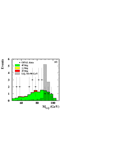
$\mu^{+}\mu^{-}{\rm qq}$

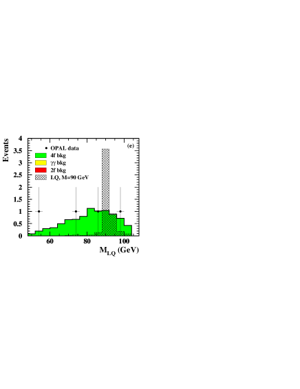
$\tau^{+}\tau^{-}{\rm qq}$

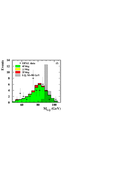
Figure 6: The leptoquark masses reconstructed by the kinematic fits used in the selections for events of classes B and C. The notation is the same as in Figure 1.

In Figure 6 the leptoquark mass reconstructed by the kinematic fits is shown for all the events surviving the selections for classes B and C, for both the background and a simulated signal. For a leptoquark mass ${\rm M_{LQ}}=90$ GeV at the centre-of-mass energy of 206 GeV the mass resolution, obtained by a Gaussian fit to the peak region, ranges from 1.3 GeV ($\mu^{+}\mu^{-}{\rm qq}$ channel) to 5.0 GeV ($\tau^{\pm}\nu{\rm qq}$ channel), while the mean value of the reconstructed mass is between 89.8 ($\tau^{\pm}\nu{\rm qq}$) and 91.6 GeV ($e^{+}e^{-}{\rm qq}$).

The detection efficiencies for the different topologies of signal events, as functions of the leptoquark mass M_LQ, are listed in Tables 10 and 11 for scalar and vector leptoquarks respectively, for the centre-of-mass energies where the signal was simulated.

MLQ (GeV)		50	60	70	75	80	85	90	95	99	102
Signal topology	Generation
		$\sqrt{s}$ = 189 GeV
Class A	1,2,3	11.4	17.7	23.9	26.9	30.2	34.4	37.4	–	–	–
Class B1	1	10.0	16.1	22.7	27.3	27.9	31.6	36.0	–	–	–
Class B1	2	13.5	22.8	29.6	33.2	35.5	39.9	41.9	–	–	–
Class B2	3	1.9	5.3	9.9	12.3	15.7	19.0	22.1	–	–	–
Class C1	1	30.2	37.4	44.5	48.2	48.3	51.6	53.7	–	–	–
Class C1	2	35.1	42.9	52.0	57.1	61.1	65.5	66.2	–	–	–
Class C2	3	20.0	26.2	31.0	30.7	34.0	33.7	35.3	–	–	–
		$\sqrt{s}$ = 196 GeV
Class A	1,2,3	10.3	16.3	22.4	26.4	28.1	30.5	33.8	37.7	–	–
Class B1	1	8.9	14.7	20.9	21.9	25.6	28.6	32.3	35.3	–	–
Class B1	2	11.7	21.2	28.6	31.3	34.2	36.7	41.3	43.5	–	–
Class B2	3	1.3	4.4	8.5	11.1	13.1	17.4	19.9	23.1	–	–
Class C1	1	28.9	36.1	41.8	45.1	49.7	51.2	53.3	54.3	–	–
Class C1	2	33.7	41.1	49.4	52.9	61.1	62.5	65.4	67.8	–	–
Class C2	3	18.7	25.7	27.8	29.1	32.2	32.8	33.1	34.4	–	–
		$\sqrt{s}$ = 200 GeV
Class A	1,2,3	9.7	15.1	21.0	23.7	26.6	29.5	32.1	34.9	38.2	–
Class B1	1	8.7	14.2	18.9	23.8	25.0	29.3	30.2	34.0	35.4	–
Class B1	2	11.4	20.7	27.7	31.2	32.8	37.0	37.8	42.5	43.1	–
Class B2	3	1.2	3.9	7.1	11.3	13.0	17.7	18.3	22.9	25.4	–
Class C1	1	27.8	35.1	39.8	44.7	46.8	48.8	51.7	54.4	55.6	–
Class C1	2	32.8	40.6	48.7	53.5	57.3	62.1	65.8	67.5	66.7	–
Class C2	3	18.0	25.0	26.9	29.4	31.7	32.0	33.3	33.6	33.6	–
		$\sqrt{s}$ = 206 GeV
Class A	1,2,3	9.1	13.5	18.9	21.1	24.8	27.4	30.2	33.4	34.2	38.1
Class B1	1	8.6	13.8	18.2	21.2	23.7	25.8	29.1	31.9	32.9	33.1
Class B1	2	10.8	20.8	25.1	28.7	32.4	34.5	36.9	38.5	39.6	41.7
Class B2	3	1.4	2.9	6.8	8.5	10.9	13.7	18.6	20.8	22.2	22.9
Class C1	1	26.0	33.8	39.5	42.6	46.8	48.0	50.0	52.9	54.1	54.4
Class C1	2	31.3	40.2	45.4	51.8	57.6	59.3	63.0	66.3	65.7	66.6
Class C2	3	16.9	25.0	25.9	29.4	31.3	32.5	32.7	35.2	34.0	34.7

Table 10: The percentage detection efficiencies for scalar leptoquarks for the various selections as functions of the leptoquark mass, M_LQ, and the centre-of-mass energy.

MLQ (GeV)		70	75	80	85	90	95	99	102
Signal topology	Generation
		$\sqrt{s}$ = 196 GeV
Class A	1,2,3	22.3	25.5	28.9	31.9	35.9	40.8	–	–
Class B1	1	17.9	21.3	27.0	29.5	31.2	33.4	–	–
Class B1	2	25.3	28.3	32.5	35.5	38.1	41.4	–	–
Class B2	3	7.9	10.3	13.8	18.3	21.6	23.7	–	–
Class C1	1	40.5	45.5	49.2	50.1	51.4	54.5	–	–
Class C1	2	49.4	55.1	59.5	62.7	64.1	66.8	–	–
Class C2	3	28.5	30.8	32.4	33.8	34.9	33.9	–	–
		$\sqrt{s}$ = 200 GeV
Class A	1,2,3	21.4	24.4	28.0	30.8	34.0	39.1	42.7	–
Class B1	1	17.4	19.2	25.8	29.2	30.0	33.3	33.5	–
Class B1	2	24.5	26.9	31.4	34.8	36.7	40.6	42.3	–
Class B2	3	7.3	9.4	12.1	17.1	20.4	23.4	23.9	–
Class C1	1	39.1	44.1	48.8	49.9	50.5	52.9	56.3	–
Class C1	2	47.7	53.8	58.1	62.4	63.3	65.6	68.0	–
Class C2	3	27.8	30.2	32.0	33.2	35.0	34.7	33.0	–
		$\sqrt{s}$ = 206 GeV
Class A	1,2,3	19.8	22.0	25.3	28.5	32.4	34.4	37.6	41.1
Class B1	1	16.1	17.9	22.3	24.7	26.9	30.9	32.4	31.9
Class B1	2	21.5	26.5	29.6	31.3	34.7	38.9	40.4	40.7
Class B2	3	6.3	8.9	11.7	14.2	17.4	21.1	22.4	24.4
Class C1	1	40.5	43.4	47.1	48.6	50.7	51.3	54.1	54.6
Class C1	2	46.2	51.0	55.6	60.0	62.6	66.6	66.4	67.2
Class C2	3	27.0	28.1	31.0	34.0	33.9	34.0	35.1	34.2

Table 11: Same as Table 10, but for vector leptoquarks.

The systematic uncertainty on the signal efficiency is evaluated to be 8–31$\%$ depending on the signal topology and the leptoquark mass. This is estimated by taking into account the following sources (the quoted errors are relative):

• The statistical uncertainty due to the limited number of simulated signal events lies in the range of 1–28$\%$.

• In the region between two simulated leptoquark masses, the value of the efficiency is calculated by a linear interpolation. The error associated with this procedure is estimated to be 2–8$\%$.

• The uncertainty introduced by the Monte Carlo modelling of the variables used in the selections contributes a systematic error between 3 and 29%. The largest relative effects are due to the scaled energies of the muons, $E_{\mu 1}/\sqrt{s}$ and $E_{\mu 2}/\sqrt{s}$, for events of class C, second generation, (up to 28%), to the scaled lepton energies, $E_{\tau,{\rm fit}}/\sqrt{s}$ and $E_{\nu,{\rm fit}}/\sqrt{s}$, for events of class B, third generation, (up to 25%) and to the fit probability and the reconstructed leptoquark mass (up to 19%), for events of the same class. Most of the other selection variables contribute uncertainties of less than 10%.

• The error associated with the lepton identification method (3–14$\%$).

• The uncertainty due to the flavour of the final state quarks contributes an error of 2–8%. This is evaluated by comparing the efficiencies corresponding to all the final states with different quark flavours simulated for a given decay channel, characterized by the lepton flavour (for example ${\rm e^{+}e^{-}u\overline{u}}$, ${\rm e^{+}e^{-}d\overline{d}}$, ${\rm e^{+}e^{-}c\overline{c}}$, ${\rm e^{+}e^{-}s\overline{s}}$ and ${\rm e^{+}e^{-}b\overline{b}}$ for class C, first generation). The value of the efficiency is taken to be the mean value, and the largest difference between the mean and the single contributions is taken as a systematic error.

• In the range of values of the $\lambda$ couplings covered by this analysis the produced leptoquarks may hadronize before decaying. This process is not simulated by the standard signal Monte Carlo. The systematic error on the detection efficiencies associated with the fragmentation model is estimated to be 2–4$\%$, evaluated by using MC samples with pair produced scalar quarks (squarks) with R-parity violating decays. These events have features similar to events of class C but in these samples the hadronization step is simulated before the squark decay. The efficiencies obtained by applying the selection for class C to these events are compared to those obtained using the corresponding standard leptoquark samples and the differences are taken as the systematic errors. Moreover, for the classes of events where the leptoquark mass is reconstructed, the mass distributions obtained by using the different samples are also compared and the mean of the absolute value of the difference between the contents of corresponding bins in the two distributions is taken as a systematic error. This contribution is estimated to be 3–8%.

• The data sample is divided into 10 energy bins, as shown in Table 3. However the signal is not simulated at each energy. At centre-of-mass energies, $\sqrt{s}$, where no simulation exists, the efficiency for a given leptoquark mass is inferred from the sample at the nearest simulated energy, $\sqrt{s^{\prime}}$. The efficiency is assumed to be the same as the efficiency for the mass point at $\sqrt{s^{\prime}}$ with the same Lorentz boost, that is $\varepsilon(\sqrt{s},~{}\mathrm{M_{{\rm LQ}}})$= $\varepsilon(\sqrt{s^{\prime}},~{}\sqrt{s^{\prime}/s}~{}\mathrm{M_{{\rm LQ}}})$. The error associated with this assumption is calculated by comparing the efficiencies obtained for corresponding masses at the energies at which the signal is simulated. The difference is taken as the error and it is found to be 2–7%.

The polarization of tau leptons from leptoquark decay is not considered in the simulation of tau decay in the signal events belonging to $\tau^{+}\tau^{-}{\rm qq}$ and $\tau^{\pm}\nu{\rm qq}$ channels. However it has been checked that the effect on the detection efficiencies for vector leptoquarks is negligible. All the above errors are considered to be independent and added in quadrature.

For the purpose of setting limits, the events are divided into different search channels by considering their centre-of-mass energy, the decay channel and, for events of classes B and C, the reconstructed leptoquark mass divided into 1 GeV bins. The confidence level for the existence of a signal is calculated following the method described in [31]. A test statistic is defined which expresses how signal-like the data are. The confidence levels are computed from the value of the test statistic of the observed data and its expected distributions in a large number of simulated experiments under two hypotheses: the background-only ($b$) hypothesis and the signal+background ($s+b$) hypothesis.

The test statistic chosen is the likelihood ratio, $Q$, the ratio of the probability of observing the data given the $s+b$ hypothesis to the probability of observing the data given the $b$ hypothesis. As all the search channels are considered to be statistically independent and to obey Poisson statistics, the likelihood ratio can be computed as

$\displaystyle Q={\rm e}^{-s_{{\rm tot}}}\prod_{i}(1+s_{i}/b_{i})^{n_{i}}$

where $n_{i}$, $b_{i}$ and $s_{i}$ are the number of observed candidates, the expected background and the expected signal in channel $i$ respectively and $s_{{\rm tot}}=\sum_{i}s_{i}$.

The confidence level for the $b$ hypothesis is $1-{\rm CL}_{b}$, representing the fraction of background-only experiments which would produce a value of $Q$ more signal-like than the observed data:

$1-{\rm CL}_{b}=P(Q>Q_{obs}|b)$.

If the data agreed perfectly with the expectation from the background-only hypothesis, a value of $1-{\rm CL}_{b}=0.5$ would be obtained. A lower value indicates an excess of events in the data; a higher value indicates a deficit. Similarly, the agreement of the data with the $s+b$ hypothesis is tested by the confidence level CL_s+b, defined as

CL${}_{s+b}=P(Q\leq Q_{obs}|s+b)$

which can be used to exclude the $s+b$ hypothesis when it has a small value. However, in the case of a large downward fluctuation of the observed background, this procedure may exclude a signal for which there is no sensitivity.

To reduce this possibility the ratio

${\rm CL}_{s}={\rm CL}_{s+b}/{\rm CL}_{b}$

is used to set limits instead. A signal is therefore considered excluded at the 95$\%$ confidence level if ${\rm CL}_{s}<0.05$.

The expected signal $s_{i}$ depends on the electroweak quantum numbers of each leptoquark and on the unknown leptoquark mass. The assumption is made that for each scenario only one state contributes to the cross-section. Therefore, for each state in the model, ${\rm CL}_{s}$ and $1-{\rm CL}_{b}$ must be calculated as a function of M_LQ. In the cases of $S_{0}(-1/3)$, $S_{1/2}(-2/3)$, $V_{0}(-2/3)$ and $V_{1/2}(-1/3)$ the value of the branching ratio into a charged lepton and a quark, $\beta$, is not predicted in the model either and exclusion limits are therefore functions of both M_LQ and $\beta$.

The statistical and systematic uncertainties on the expected number of events both for signal and background are incorporated in the calculations of the confidence levels as suggested in [32]. The probability of observing $n_{i}$ events in channel $i$, and the corresponding value of the test-statistic $Q$, are integrated over possible values of $s_{i}$ and $b_{i}$ given by their uncertainties, assuming Gaussian distributions, with a lower tail cut-off at zero, so that negative $s_{i}$ or $b_{i}$ are not allowed. In this approach the errors on $s_{i}$ and $b_{i}$ within a channel and between channels are considered to be uncorrelated.

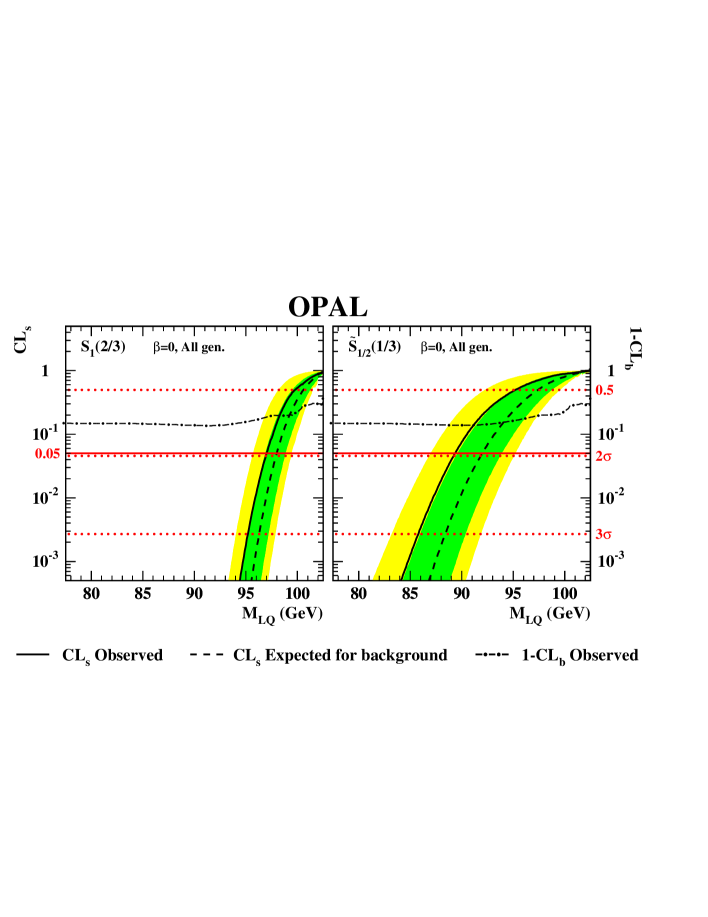
Figure 7: The value of CL_s as a function of the mass, for scalar leptoquarks $S_{1}(2/3)$ and $\tilde{S}_{1/2}(1/3)$ with $\beta=0$. The observations for the data are shown with solid lines. The shaded bands indicate the 68% and 95% probability intervals with respect to the median expectation in the absence of a signal (dashed lines). The mass values corresponding to the intersection of the observed CL_s with the horizontal solid line at CL${}_{s}=0.05$ represent the exclusion limits at 95$\%$ CL. The dash-dotted line shows the observed values for the Confidence Level $1-{\rm CL}_{b}$; its median expectation in the background hypothesis (0.5) and the levels for $2\sigma$ and $3\sigma$ deviations from this value correspond to the horizontal dotted lines.

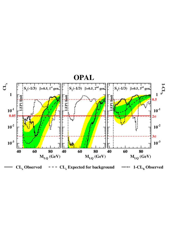
Figure 8: Same as Figure 7, but for $S_{1}(-1/3)$ with $\beta=0.5$.

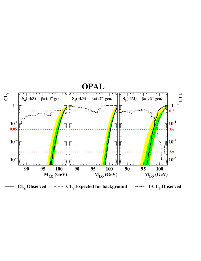
Figure 9: Same as Figure 7, but for $\tilde{S}_{0}(-4/3)$ with $\beta=1$.

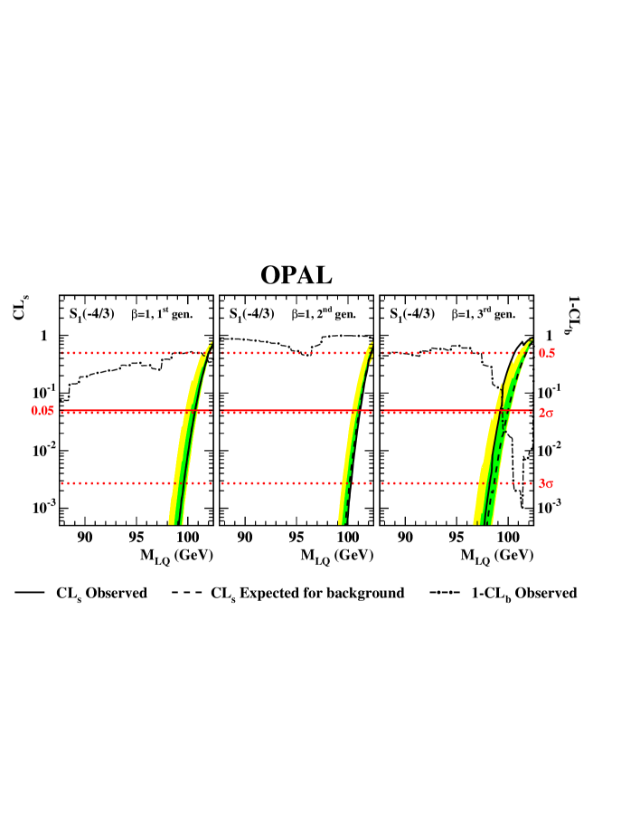
Figure 10: Same as Figure 7, but for $S_{1}(-4/3)$ with $\beta=1$.

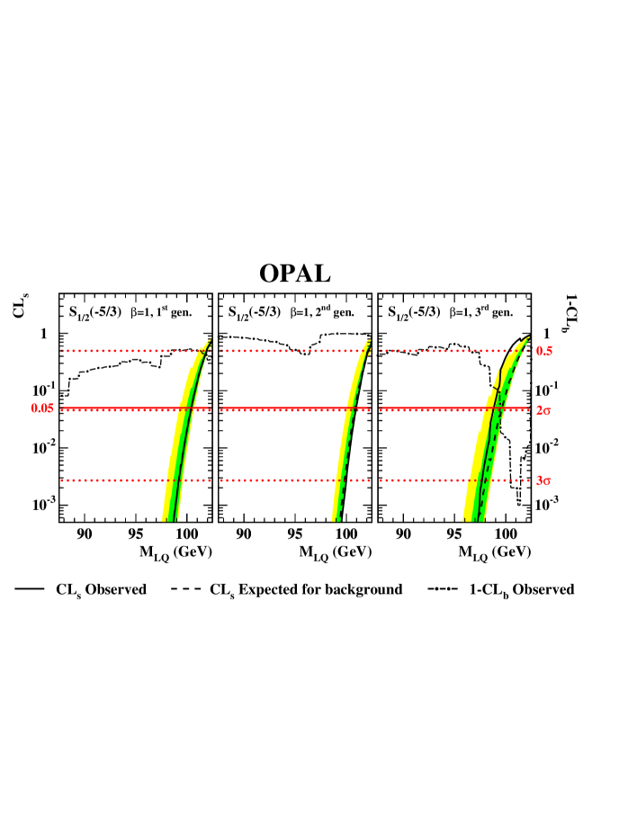
Figure 11: Same as Figure 7, but for $S_{1/2}(-5/3)$ with $\beta=1$.

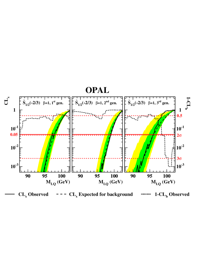
Figure 12: Same as Figure 7, but for $\tilde{S}_{1/2}(-2/3)$ with $\beta=1$.

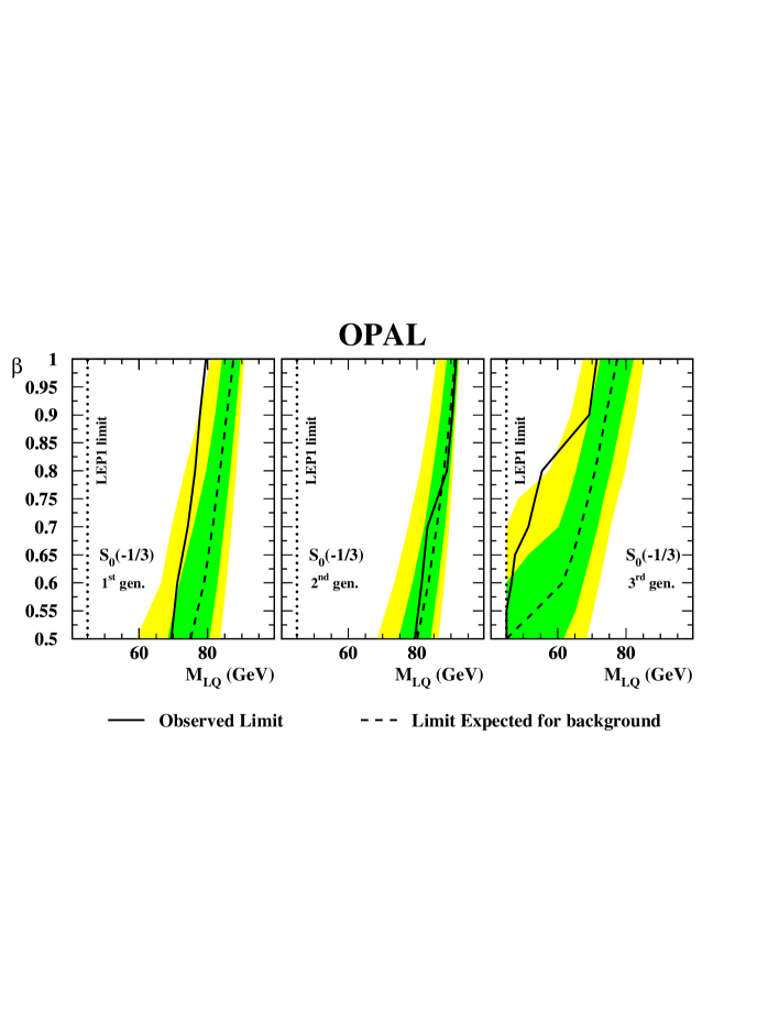
Figure 13: The 95$\%$ CL exclusion curves in the plane $\beta$ vs M_LQ for $S_{0}(-1/3)$ with possible values of $\beta$ in the range $\left[0.5,1\right]$. The observations for the data are shown with solid lines. The shaded bands indicate the 68% and 95% probability intervals with respect to the median expectation in the absence of a signal (dashed lines). The excluded region is to the left of the solid curve.

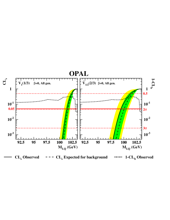
Figure 15: Same as Figure 7, but for vector leptoquarks $V_{1}(1/3)$ and $\tilde{V}_{1/2}(2/3)$ with $\beta=0$.

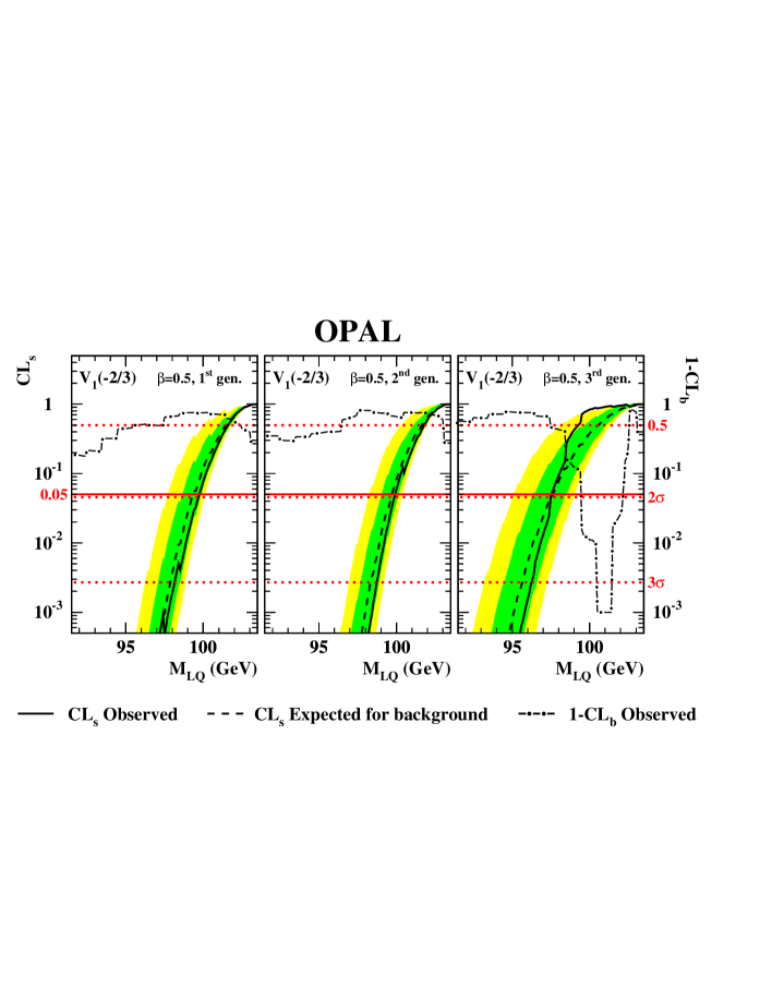
Figure 16: Same as Figure 15, but for $V_{1}(-2/3)$ with $\beta=0.5$.

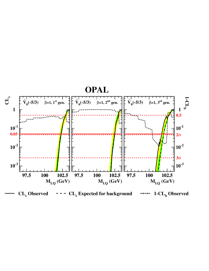
Figure 17: Same as Figure 15, but for $\tilde{V}_{0}(-5/3)$ with $\beta=1$.

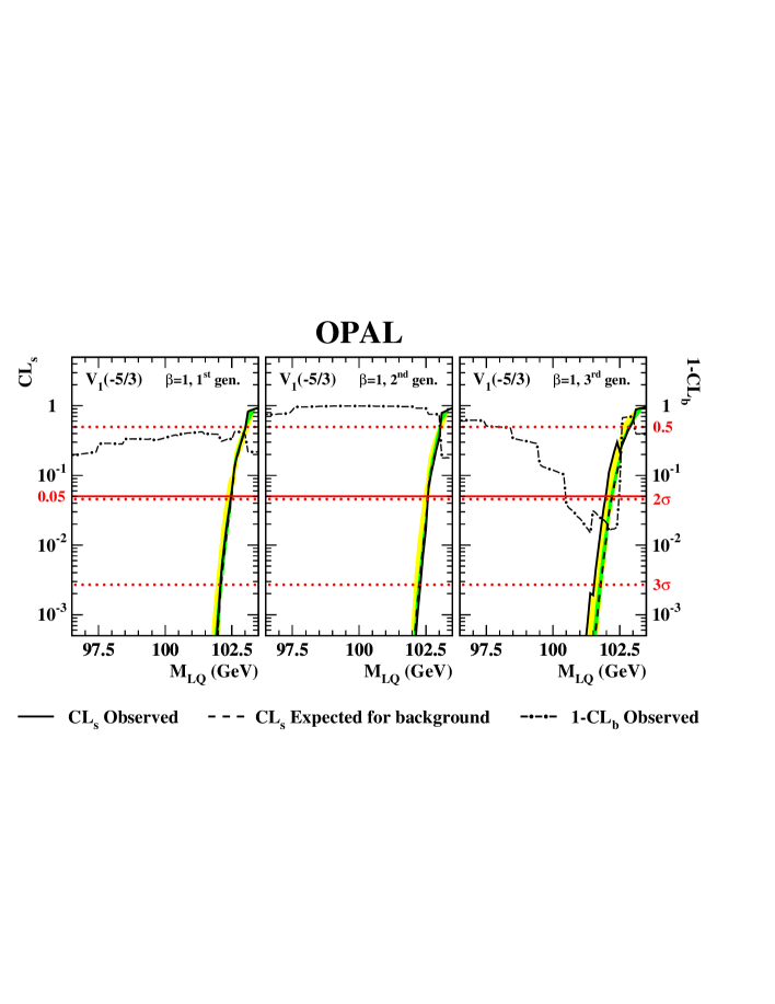
Figure 18: Same as Figure 15, but for $V_{1}(-5/3)$ with $\beta=1$.

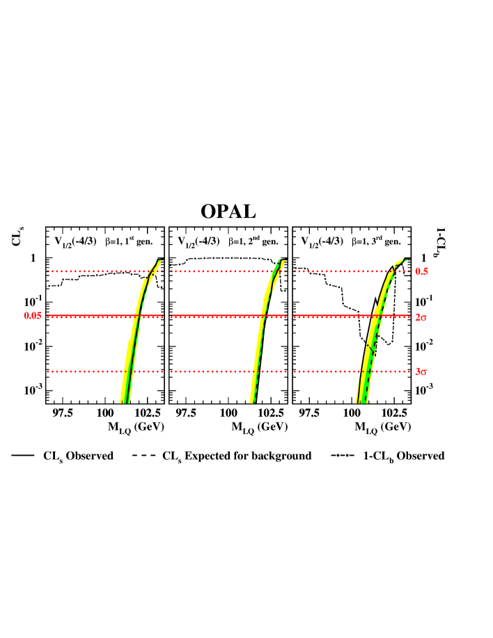
Figure 19: Same as Figure 15, but for $V_{1/2}(-4/3)$ with $\beta=1$.

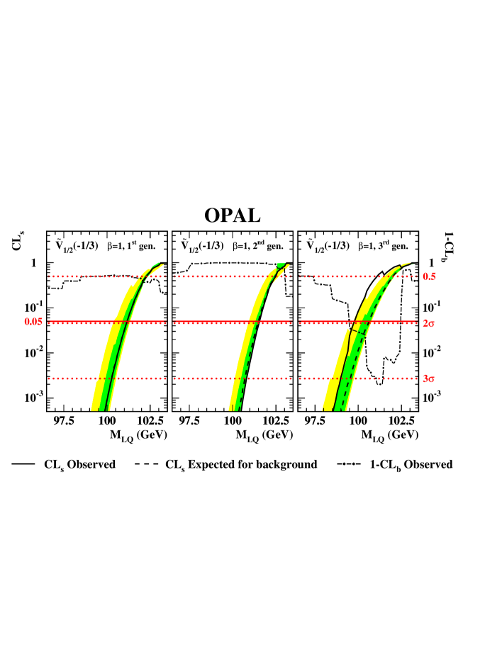
Figure 20: Same as Figure 15, but for $\tilde{V}_{1/2}(-1/3)$ with $\beta=1$.

Figures 7–12 and 15–20 show the values of CL_s as a function of the leptoquark mass, M_LQ, for scalar and vector leptoquarks with the branching ratio $\beta$ predicted in the model. The lower limit at the 95$\%$ CL on M_LQ corresponds to the intersection with the line at CL${}_{s}=0.05$. In the same figures the curves representing the values of $1-{\rm CL}_{b}$ are also shown. In a Gaussian approximation a value $1-{\rm CL}_{b}=4.55\times 10^{-2}$ would indicate a $2\sigma$ excess beyond the background median expectation and $1-{\rm CL}_{b}=2.7\times 10^{-3}$ would indicate a $3\sigma$ excess. The vertical scales on the right-hand side of Figures 7–12 and 15–20 correspond to this approximation. The regions excluded in the $\beta-{\rm M}_{\mathrm{LQ}}$ plane of the states $S_{0}$, $S_{1/2}(-2/3)$, $V_{0}$ and $V_{1/2}(-1/3)$, whose $\beta$ depend on the relative weights of the unknown left and right $\lambda$ couplings, are shown in Figures 13, 14, 21 and 22. The mass limits obtained are summarized in Table 12. Because of the very small cross-section and the lower efficiency of the selection for the $\tau^{\pm}\nu{\rm qq}$ channel, this search can only improve previous lower limits on the mass of the third generation state $S_{0}(-1/3)$ over a part of the $\beta$ range, while for the third generation state $S_{1}(-1/3)$ with $\beta=0.5$ no improvement is possible.

$\mathrm{LQ}$		$Q_{{\rm em}}$		$\beta$	Generation
					1		2		3
$S_{0}$		-1/3		[0.5,1]	69		79		45$(\ast)$
$\tilde{S}_{0}$		-4/3		1	99		100		98
		2/3		0	$\longleftarrow---$		97	$---\longrightarrow$
$S_{1}$		-1/3		0.5	69		79		45$(\ast)$
		-4/3		1	100		101		99
		-2/3		[0,1]	94		94		93
$S_{1/2}$
		-5/3		1	100		100		98
		1/3		0	$\longleftarrow---$		89	$---\longrightarrow$
$\tilde{S}_{1/2}$
		-2/3		1	97		99		96
$V_{0}$		-2/3		[0.5,1]	99		99		97
$\tilde{V}_{0}$		-5/3		1	102		102		101
		1/3		0	$\longleftarrow---$		101	$---\longrightarrow$
$V_{1}$		-2/3		0.5	99		99		97
		-5/3		1	102		102		101
		-1/3		[0,1]	99		99		98
$V_{1/2}$
		-4/3		1	102		102		101
		2/3		0	$\longleftarrow---$		99	$---\longrightarrow$
$\tilde{V}_{1/2}$
		-1/3		1	101		101		99

Table 12: The $95\%$ CL lower limits on scalar and vector leptoquarks masses, in GeV, as obtained from the present analysis. $\beta$ is the branching ratio into a charged lepton and a quark. Limits obtained by OPAL using LEP1 data are marked with ($\ast$).

6 Conclusions

The data collected with the OPAL detector at $\sqrt{s}$ between 189 and 209 GeV, corresponding to a total integrated luminosity of 596 pb^-1, are analysed to search for events with pair produced leptoquarks of all three generations. The present analysis covers the region of small values of the couplings $\lambda$ to fermions (from 10^-6 to 10^-2). No significant signal-like excess with respect to Standard Model predictions is found in the data. Lower mass limits are set for scalar and vector leptoquarks under the assumption that, for each scenario, only one leptoquark state contributes to the cross-section. The present results improve most of the previous LEP lower limits on leptoquark masses derived from searches for events due to the pair production process [7, 8] by 10–25 GeV, depending on the leptoquark quantum numbers.

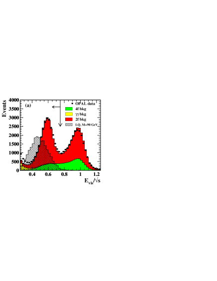
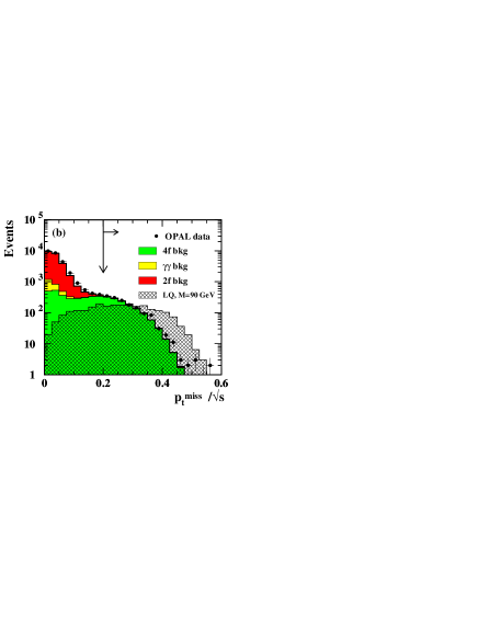
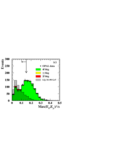
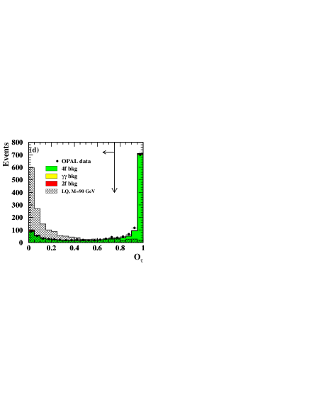
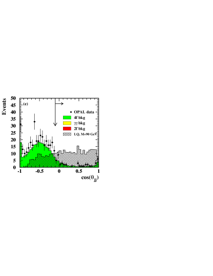
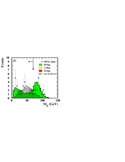
Figure 1: Class A, the $\nu\nu{\rm qq}$ channel: distributions of the selection variables for the data (points with bars denoting the statistical error), the estimated Standard Model background (filled histogram) and a simulated signal (hatched histogram), with arbitrary normalization, corresponding to scalar leptoquarks of mass M${}_{\mathrm{LQ}}=90$ GeV at $\sqrt{s}=206$ GeV. All the distributions are shown for the events surviving all the cuts applied before the cut on the plotted variable, following the description of the selection in the text. The arrows indicate the positions of the cuts and the accepted regions.
(a) The scaled visible energy. (b) The scaled transverse missing momentum. (c) The scaled energy of the most energetic lepton (electron or muon), if a lepton is found. (d) The output from the neural net, $\cal{O}_{\tau}$, for the tau with the highest value in the event, after cut (A-2). (e) The cosine of the angle between the two reconstructed jets, $\theta_{{\rm jj}}$. (f) The invariant mass of the two reconstructed jets, ${\rm M_{jj}}$.

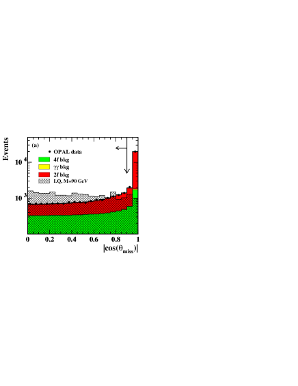
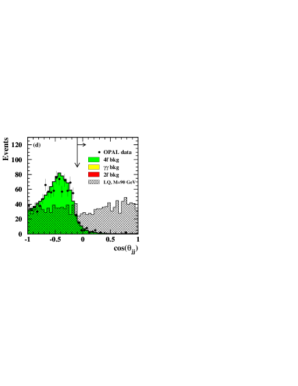
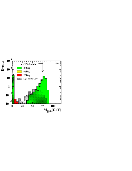
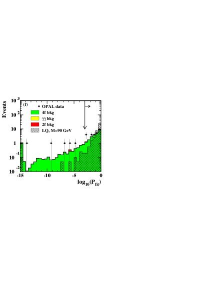
Figure 2: Class B1, the $l^{\pm}\nu{\rm qq}$ channel: same as Figure 1, but for class B1. All the distributions refer to the selection for second generation leptoquarks.
(a) The absolute value of the cosine of  $\theta_{{\rm miss}}$, the angle between the direction of the missing momentum and the $z$-axis. (b) The scaled energy of the most energetic lepton (${\mu}$ or $\nu$). (c) The angle between the direction of the most energetic muon in the event and the nearest charged track. (d) The cosine of the angle between the directions of the two reconstructed jets, $\theta_{jj}$. (e) The invariant mass, ${\rm M_{jj,fit}}$, of the jet-jet system reconstructed by the kinematic fit described in cut (B1-7). The first bin also contains the events failing the fit or with a probability smaller than 0.1. (f) The logarithm of the fit probability, P_fit, used to reconstruct the leptoquark mass. The first bin also contains the events failing the fit or with a probability smaller than $10^{-15}$.

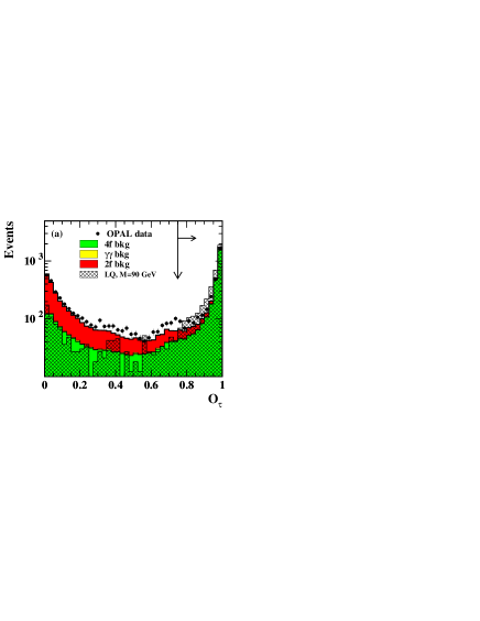
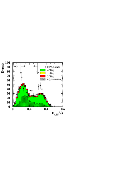
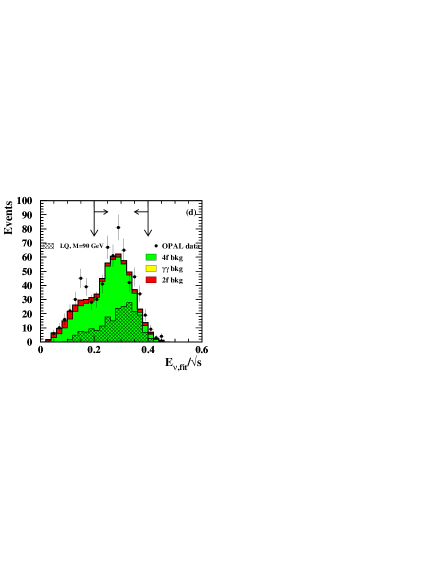
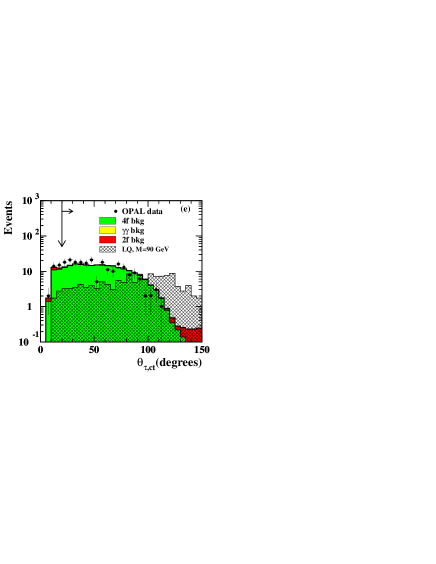
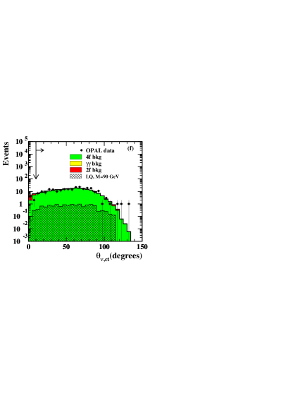
Figure 3: Class B2, the $\tau^{\pm}\nu{\rm qq}$ channel: same as Figure 1, but for class B2.
(a) The output $\mathcal{O}_{\tau}$ from the neural network algorithm, for the tau with the highest output in the event. (b) The invariant mass, ${\rm M_{jj,fit}}$ of the jet-jet system reconstructed by the first kinematic fit described in cut (B2-5). The first bin contains also the events failing the fit or with a probability smaller than 0.1. (c)–(d) The scaled energies of the tau lepton and the neutrino, $E_{\tau,{\rm fit}}/\sqrt{s}$ and $E_{\nu,{\rm fit}}/\sqrt{s}$, as calculated by the kinematic fit used to reconstruct the leptoquark mass, after cut (B2-5). (e)–(f) The angles between the leptons and the nearest charged track for the tau, $\theta_{\tau,{\rm ct}}$, and the neutrino, $\theta_{\nu,{\rm ct}}$, respectively, after cut (B2-6).

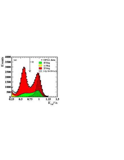
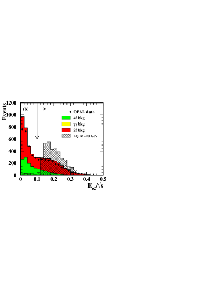
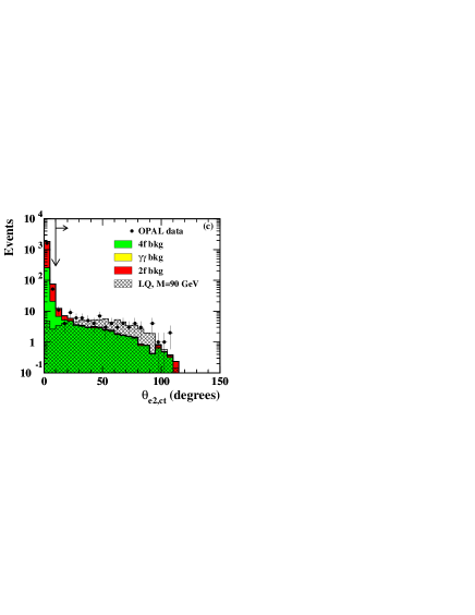
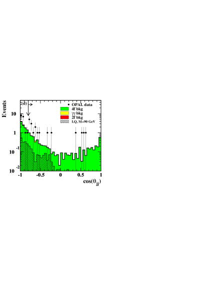
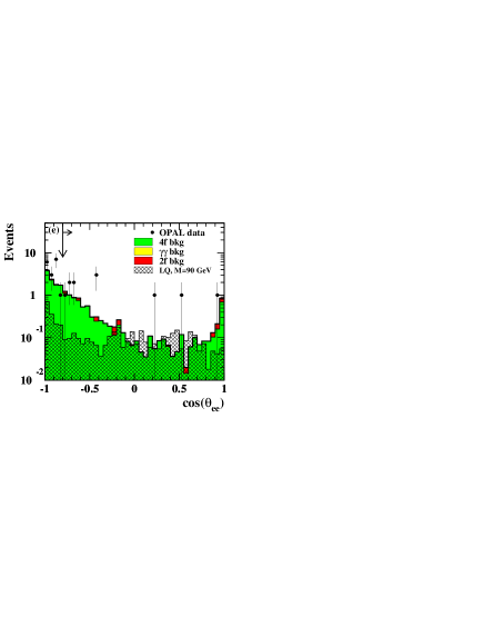
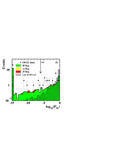
Figure 4: Class C1, the $l^{+}l^{-}{\rm qq}$ channel: same as Figure 1, but for class C1. All the distributions refer to the selection for first generation leptoquarks.
(a) The scaled visible energy. (b) The scaled energy of the second most energetic electron in the event, after cut (C1-2). (c) The angle between the second most energetic electron and the nearest charged track, after (C1-3). (d) The cosine of $\theta_{{\rm jj}}$, the angle between the two reconstructed jets, after cut (C1-4). The distribution does not contain the events with $\cos(\theta_{{\rm ee}})>-0.8$, which are always selected by cut (C1-5), independently of the value of $\cos(\theta_{{\rm jj}})$. (e) The cosine of $\theta_{{\rm ee}}$, the angle between the two most energetic electrons, after cut (C1-4). The distribution does not contain the events with $\cos(\theta_{{\rm jj}})>-0.8$, which are always selected by cut (C1-5), independently of the value of $\cos(\theta_{{\rm ee}})$. (f) The logarithm of the probability of the fit used to reconstruct the leptoquark mass. The first bin contains also the events failing the fit or with a probability smaller than $10^{-15}$.

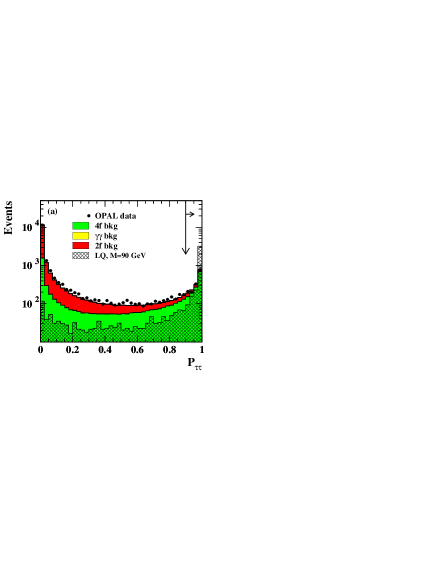
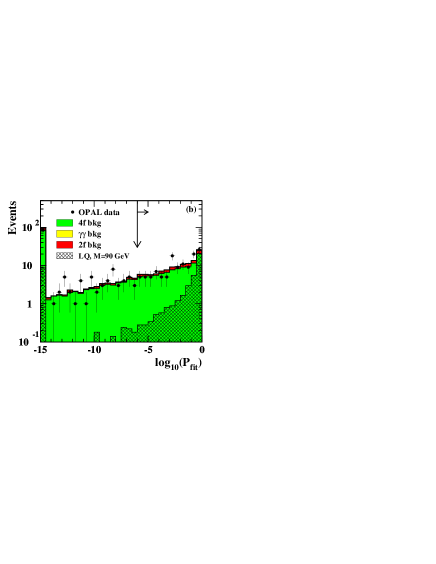
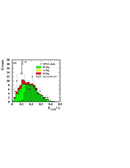
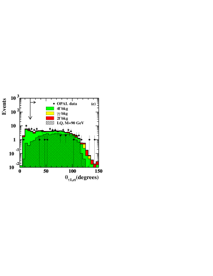
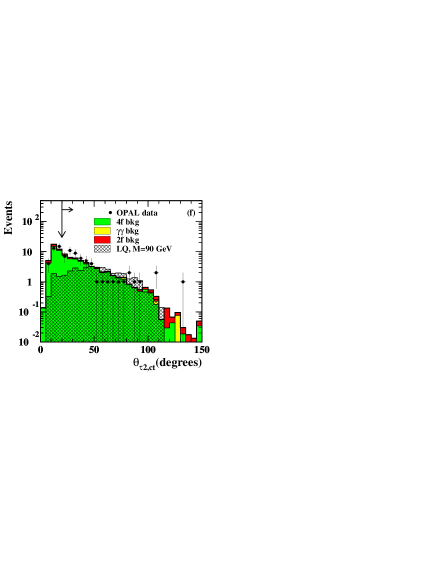
Figure 5: Class C2, the $\tau^{+}\tau^{-}{\rm qq}$ channel: same as Figure 1, but for class C2.
(a) The two-tau probability, $\cal{P}_{\tau\tau}$, defined in cut (C2-3). (b) The logarithm of the probability of the kinematic fit used to reconstruct the leptoquark mass. The first bin contains also the events failing the fit or with a probability lower than 10^-15. (c)-(d) The scaled energies of the most energetic and of the second most energetic tau in the event respectively, after cut (C2-4). (e)-(f) The angles between the direction of the momenta of the most energetic and the second most energetic tau leptons and the nearest charged track, respectively, after cut (C2-5).

${\rm e}^{\pm}\nu{\rm qq}$

$\mu^{\pm}\nu{\rm qq}$

$\tau^{\pm}\nu{\rm qq}$

${\rm e}^{+}{\rm e}^{-}{\rm qq}$

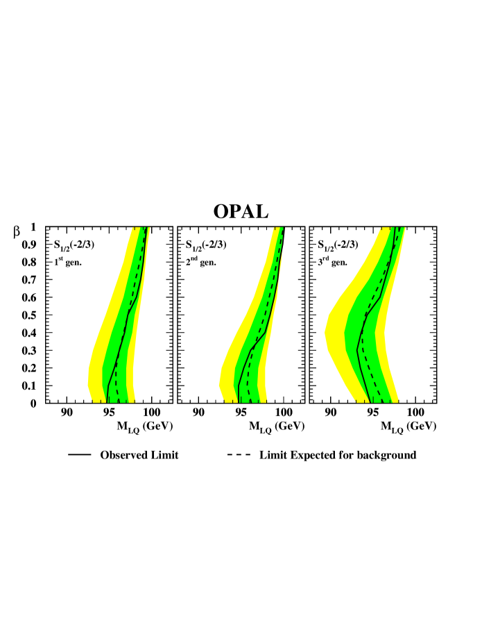
Figure 14: Same as Figure 13, but for ${S}_{1/2}(-2/3)$ with possible values of $\beta$ in the range $\left[0,1\right]$.

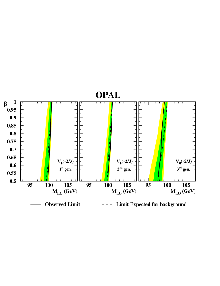
Figure 21: Same as Figure 13, but for vector leptoquark $V_{0}(-2/3)$ with possible values of $\beta$ in the range $\left[0.5,1\right]$.

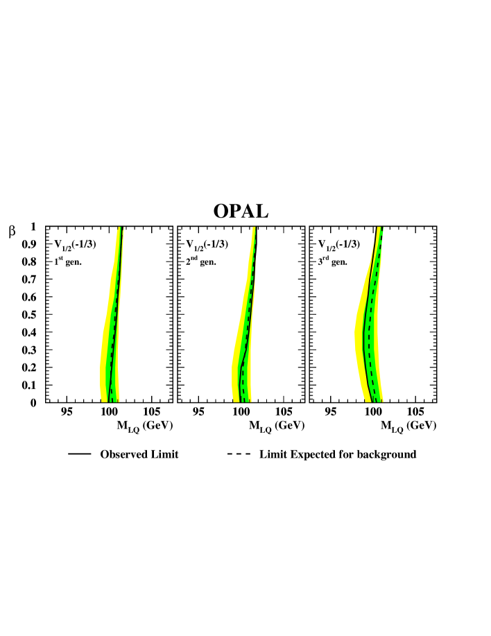
Figure 22: Same as Figure 21, but for ${V}_{1/2}(-1/3)$ with possible values of $\beta$ in the range $\left[0,1\right]$.

References

-
[1]
J.C. Pati and A. Salam, Phys. Rev. D10 (1974) 275;
E. Farhi and L. Susskind, Phys. Rep. 74 (1981) 277;
B. Schrempp and F. Schrempp, Phys. Lett. B153 (1985) 101;
J.L. Hewett and T.G. Rizzo, Phys. Rep. 183 (1989) 193;
P.H. Frampton, Mod. Phys. Lett. A7 (1992) 559;
J.L. Hewett and T.G. Rizzo, Phys. Rev. D58 (1998). - [2] W. Buchmüller, R. Rückl and D. Wyler, Phys. Lett. B191 (1987) 442.
- [3] S. Davidson, D. Bailey and B.A. Campbell, Z. Phys. C61 (1994) 613.
-
[4]
H. Dreiner,
“An Introduction to Explicit R-parity Violation”,
in “Perspectives on Supersymmetry”, ed. G.L. Kane (1997) 462. -
[5]
ZEUS Collab., M. Derrick et al., Phys. Lett. B306 (1993) 173;
H1 Collab., I. Abt et al., Nucl. Phys. B396 (1993) 3;
H1 Collab., C. Adloff et al., Eur. Phys. J. C11 (1999) 447;
H1 Collab., C. Adloff et al., Phys. Lett. B479 (2000) 358;
H1 Collab., C. Adloff et al., Phys. Lett. B523 (2001) 234. -
[6]
DELPHI Collab., P. Abreu et al., Phys. Lett. B446 (1999) 62;
OPAL Collab., G. Abbiendi et al., Eur. Phys. J. C23 (2002) 1;
OPAL Collab., G. Abbiendi et al., Phys. Lett. B526 (2002) 233. -
[7]
OPAL Collab., G. Alexander et al., Phys. Lett. B263 (1991) 123;
L3 Collab., B. Adeva et al., Phys. Lett. B261 (1991) 169;
DELPHI Collab., P. Abreu et al., Phys. Lett. B275 (1992) 222;
ALEPH Collab., D. Decamp et al., Phys. Rep. 216 (1992) 253. - [8] OPAL Collab., G. Abbiendi et al., Eur. Phys. J. C13 (2000) 15.
-
[9]
CDF Collab., F. Abe et al., Phys. Rev. Lett. 79 (1997) 4327;
CDF Collab., F. Abe et al., Phys. Rev. Lett. 81 (1998) 4806;
CDF Collab., B. Abbott et al., Phys. Rev. Lett. 83 (1999) 2896;
CDF Collab., B. Abbott et al., Phys. Rev. Lett. 84 (2000) 2088;
CDF Collab., T. Affolder et al., Phys. Rev. Lett. 85 (2000) 2056;
D0 Collab., S. Abachi et al., Phys. Rev. Lett. 80 (1998) 2051;
D0 Collab., S. Abachi et al., Phys. Rev. Lett. 81 (1998) 38;
D0 Collab., V.M. Abazov et al., Phys. Rev. D64 (2001) 092004;
D0 Collab., V.M. Abazov et al., Phys. Rev. Lett. 88 (2002) 191801. -
[10]
J. Blümlein and R. Rückl, Phys. Lett. B304 (1993) 337;
J. Blümlein and E. Boos, Nucl. Phys. (Proc. Suppl.) B37 (1994) 181. - [11] OPAL Collab., K. Ahmet et al., Nucl. Instr. and Meth. A305 (1991) 275.
- [12] S. Anderson et al., Nucl. Instr. and Meth. A403 (1998) 326.
- [13] B.E. Anderson et al., IEEE Transactions on Nuclear Science 41 (1994) 845.
- [14] G. Aguillon et al., Nucl. Instr. and Meth. A417 (1998) 266.
-
[15]
D.M. Gingrich, in “Physics at LEP2”, CERN 96-01,
eds. G. Altarelli, T. Sjöstrand and F. Zwirner, Vol. 2, 345. -
[16]
T. Sjöstrand, Comput. Phys. Commun. 39 (1986) 347;
T. Sjöstrand, PYTHIA 5.7 and JETSET7.4 Manual, CERN-TH 7112/93. - [17] S. Jadach et al, Comput. Phys. Commun. 130 (2000) 260.
- [18] G. Marchesini et al., Comput. Phys. Commun. 67 (1992) 465.
-
[19]
R. Engel and J. Ranft, Phys. Rev. D54 (1996) 4244;
R. Engel, Z. Phys. C66 (1995) 203. -
[20]
F.A. Berends, P.H. Daverveldt and R. Kleiss,
Nucl. Phys. B253 (1985), 421;
Comput. Phys. Commun. 40 (1986), 271, 285, 309. - [21] J. Fujimoto et al., Comput. Phys. Commun. 100 (1997) 128.
- [22] S. Jadach et al, Comput. Phys. Commun. 119 (1999) 272.
- [23] S. Jadach, B.F.L. Ward and Z. Wa̧s, Comput. Phys. Commun. 79 (1994) 503.
- [24] J.A.M. Vermaseren, Nucl. Phys. B229 (1983) 347.
- [25] J. Allison et al., Nucl. Instr. and Meth. A317 (1992) 47.
- [26] OPAL Collab., K. Ackerstaff et al., Eur. Phys. J. C2 (1998) 213.
- [27] OPAL Collab., K. Ackerstaff et al., Phys. Lett. B389 (1996) 416.
- [28] OPAL Collab., G. Abbiendi et al., Eur. Phys. J. C7 (1999) 407.
- [29] S. Catani et al., Phys. Lett. B269 (1991) 432.
- [30] G.J. Feldman and R.D. Cousins, Phys. Rev. D57 (1998) 3873.
- [31] OPAL Collab., G. Abbiendi et al., Phys. Lett. B499 (2001) 38.
- [32] T. Junk, Nucl. Instr. and Meth. A434 (1999) 435.