Measurements of $\Xi_{c}^{+}$ Branching Ratios

Abstract

Using data collected by the fixed target Fermilab experiment FOCUS, we measure the branching ratios of the Cabibbo favored decays $\Xi_{c}^{+}\rightarrow\Sigma^{+}K^{-}\pi^{+}$, $\Xi_{c}^{+}\rightarrow\Sigma^{+}\bar{K}^{*}(892)^{0}$, and $\Xi_{c}^{+}\rightarrow\Lambda^{0}K^{-}\pi^{+}\pi^{+}$ relative to $\Xi_{c}^{+}\rightarrow\Xi^{-}\pi^{+}\pi^{+}$ to be $0.91\pm 0.11\pm 0.04$, $0.78\pm 0.16\pm 0.06$, and $0.28\pm 0.06\pm 0.06$, respectively. We report the first observation of the Cabibbo suppressed decay $\Xi_{c}^{+}\rightarrow\Sigma^{+}K^{+}K^{-}$ and we measure the branching ratio relative to $\Xi_{c}^{+}\rightarrow\Sigma^{+}K^{-}\pi^{+}$ to be $0.16\pm 0.06\pm 0.01$. We also set 90% confidence level upper limits for $\Xi_{c}^{+}\rightarrow\Sigma^{+}\phi$ and $\Xi_{c}^{+}\rightarrow\Xi^{*}(1690)^{0}(\Sigma^{+}K^{-})K^{+}$ relative to $\Xi_{c}^{+}\rightarrow\Sigma^{+}K^{-}\pi^{+}$ to be 0.12 and 0.05, respectively. We find an indication of the decays $\Xi_{c}^{+}\rightarrow\Omega^{-}K^{+}\pi^{+}$ and $\Xi_{c}^{+}\rightarrow\Sigma^{*}(1385)^{+}\bar{K}^{0}$ and set 90% confidence level upper limits for the branching ratios with respect to $\Xi_{c}^{+}\rightarrow\Xi^{-}\pi^{+}\pi^{+}$ to be 0.12 and 1.72, respectively. Finally, we determine the 90% C.L. upper limit for the resonant contribution $\Xi_{c}^{+}\rightarrow\Xi^{*}(1530)^{0}\pi^{+}$ relative to $\Xi_{c}^{+}\rightarrow\Xi^{-}\pi^{+}\pi^{+}$ to be 0.10.

The FOCUS Collaboration

1 Introduction

In addition to several improved measurements of $\Xi_{c}^{+}$ branching ratios, we report an indication of new $\Xi_{c}^{+}$ decay modes and the first observation of the Cabibbo suppressed decay $\Xi_{c}^{+}\rightarrow\Sigma^{+}K^{+}K^{-}$. These analyses may provide useful information about the various charm baryon weak decay mechanisms. In particular we find a suggestion of the decay $\Xi_{c}^{+}\rightarrow\Sigma^{*}(1385)^{+}\bar{K}^{0}$ for which flavor symmetry arguments predict a zero amplitude [1]. A non-vanishing amplitude could be related to spin-spin interactions between the light quarks in the baryon $\Xi_{c}^{+}$ [2]. As regards the $\Xi_{c}^{+}\rightarrow\Sigma^{+}K^{+}K^{-}$, we measure the branching ratio relative to the Cabibbo favored mode $\Xi_{c}^{+}\rightarrow\Sigma^{+}K^{-}\pi^{+}$. While tree diagrams (internal and external spectator) contribute to both Cabibbo favored and Cabibbo suppressed modes, the W-exchange diagram contributes only to the Cabibbo suppressed decay (Fig. 1). Assuming a similar contribution from strong interactions for the two modes, and neglecting possible resonant structure, one might naively extract information on the role of the W-exchange diagram. This result may also aid in understanding the discrepancy between the predicted and measured $\Xi_{c}^{+}$ lifetime [3, 4].

Figure 1: Possible weak diagrams for a) and b): Cabibbo favored decay $\Xi_{c}^{+}\rightarrow\Sigma^{+}K^{-}\pi^{+}$; c), d), e): Cabibbo suppressed decay $\Xi_{c}^{+}\rightarrow\Sigma^{+}K^{+}K^{-}$. The W-exchange diagram contributes only to the Cabibbo suppressed decay.

2 Event Reconstruction

FOCUS is a photoproduction experiment which collected data during the 1996–1997 fixed-target run at Fermilab. The apparatus is equipped with precise vertex and comprehensive particle identification detectors. For about 2/3 of the data taking a $25~{}\mu\textrm{m}$ pitch silicon strip detector (TS) [5] was interleaved with the BeO target segments. The spectrometer is divided into an inner region for high momentum track reconstruction and an outer region for low momentum tracks.

All decay modes reported have a hyperon in the final state. The $\Sigma^{+}$ particles are reconstructed in both $p$$\pi^{0}$ and $n$$\pi^{+}$ decay modes. As the direction of the neutral particle is not reconstructed, kinematic constraints are used to compute the $\Sigma^{+}$ momentum. If the decay occurs upstream of the magnetic field, there is a two-fold ambiguity in the $\Sigma^{+}$ momentum. The $\Xi^{-}$ and $\Omega^{-}$ are reconstructed in the modes $\Lambda^{0}$$\pi^{-}$ and $\Lambda^{0}$$K^{-}$, respectively, while $\Lambda^{0}$ decays are reconstructed in the charged mode $p$$\pi^{-}$. A detailed description of the hyperon reconstruction techniques in FOCUS is reported in Reference [6].

Candidates are reconstructed by first forming a vertex with tracks consistent with a specific charm decay hypothesis. A cut on the confidence level (CLD) that these tracks form a good vertex is applied. The production vertex is found using a candidate driven vertex algorithm which uses the final state momentum to define the line of flight of the charm particle [7]. The seed track for the charm particle is used to form a production vertex with at least two other tracks in the target region. We require a value of at least $1\%$ for the confidence level of the production vertex. Most of the background is rejected by applying a separation cut between the production and decay vertices (we require the significance of separation, $L/\sigma_{L}$, between the two vertices to be greater than some number). Čerenkov identification [8] is required on each charged final state particle in the decay. For each hypothesis ($\alpha=$ electron, pion, kaon or proton) we construct a $\chi^{2}$-like variable $W_{\alpha}=-2\log$ (likelihood). We use either a requirement that one hypothesis, $\beta$, is favored with respect to another hypothesis, $\alpha$, ($W_{\alpha}-W_{\beta}>n)$ or a requirement that one hypothesis is favored with respect to all the other hypotheses ($\min\{W_{\alpha}\}-W_{\beta}>n$).

In order to minimize systematic biases, the normalization mode is selected using the same cuts as the specific decay when possible. Differences between each mode and its reference mode will be discussed below. The evaluation of efficiencies accounts for the decay fractions of the observed daughters.

3 $\Xi_{c}^{+}$ decays containing a $\Sigma^{+}$ particle

We measure the branching ratio of $\Xi_{c}^{+}\rightarrow\Sigma^{+}K^{-}\pi^{+}$ and $\Xi_{c}^{+}\rightarrow\Sigma^{+}\bar{K}^{*}(892)^{0}$ relative to $\Xi_{c}^{+}\rightarrow\Xi^{-}\pi^{+}\pi^{+}$. The decay mode $\Xi_{c}^{+}\rightarrow\Sigma^{+}K^{-}\pi^{+}$ is selected by requiring $\mathrm{CLD}>1\%$ while for $\Xi_{c}^{+}\rightarrow\Xi^{-}\pi^{+}\pi^{+}$ we require $\mathrm{CLD}>2\%$. A minimum cut of $40~{}\textrm{GeV}/c$ is applied on the $\Xi_{c}^{+}$ momentum. Due to different levels of background, we require $L/\sigma_{L}>9.5$ for $\Xi_{c}^{+}\rightarrow\Sigma^{+}K^{-}\pi^{+}$ and $L/\sigma_{L}>4.5$ for $\Xi_{c}^{+}\rightarrow\Xi^{-}\pi^{+}\pi^{+}$. Each pion from the charm decay vertex must satisfy $\min\{W_{\alpha}\}-W_{\pi}>-6$. In the $\Xi_{c}^{+}\rightarrow\Sigma^{+}K^{-}\pi^{+}$ mode the kaon hypothesis must be favored over the pion hypothesis ($W_{\pi}-W_{K}>1$). To eliminate possible contamination from the $\Lambda_{c}^{+}\rightarrow\Sigma^{+}\pi^{+}\pi^{-}$ decays, where the $\pi^{-}$ is misidentified as a $K^{-}$, we increase the $K-\pi$ separation cut from 1 to 5 for those events which, reconstructed as $\Sigma^{+}\pi^{+}\pi^{-}$, fall within $30~{}\textrm{MeV}/c^{2}$ of the nominal $\Lambda_{c}^{+}$ mass. A loose requirement, $W_{p}-W_{\pi}>-3$, is applied on proton-pion separation. In addition, we reject candidates with a decay proper time resolution ($\sigma_{t}$) less than $110$ fs ($140$ fs) for TS (not TS) run period events. Further, a muon incompatibility cut is imposed on the kaon and pion for $\Xi_{c}^{+}\rightarrow\Sigma^{+}K^{-}\pi^{+}$ candidates.

Figure 2: Invariant mass distribution of: a) $\Xi_{c}^{+}\rightarrow\Sigma^{+}K^{-}\pi^{+}$. b) $\Xi_{c}^{+}\rightarrow\Xi^{-}\pi^{+}\pi^{+}$. For both modes the fit has been performed using two Gaussians for the signal and a first order polynomial for the background.

In Fig. 2 the invariant mass distributions for $\Sigma^{+}K^{-}\pi^{+}$ and $\Xi^{-}\pi^{+}\pi^{+}$ are presented. A good fit function to our data is two Gaussian distributions for the signal and a first order polynomial for the background, especially for decays with a two-fold ambiguity. For the $\Sigma^{+}K^{-}\pi^{+}$ mode the fit returns a yield of $251\pm 23$ events. For this mode, the sigmas and the ratio of the yields of the two Gaussians, and the mean of the wide Gaussian are fixed to the Monte Carlo values. The $\Xi^{-}\pi^{+}\pi^{+}$ distribution is also fit using two Gaussians for the signal and a first order polynomial for the background. The resultant yield is $265\pm 21$ events. A Monte Carlo simulation is used to determine the relative efficiency. We find no significant change in the $\Xi_{c}^{+}\rightarrow\Sigma^{+}K^{-}\pi^{+}$ efficiency due to the $\Xi_{c}^{+}\rightarrow\Sigma^{+}K^{*}(892)^{0}$ contribution. We determine the branching ratio to be

$$\frac{\Gamma(\Xi_{c}^{+}\rightarrow\Sigma^{+}K^{-}\pi^{+})}{\Gamma(\Xi_{c}^{+}\rightarrow\Xi^{-}\pi^{+}\pi^{+})}=0.91\pm 0.11~{}\textrm{(stat)}.$$ (1)

For the $\Xi_{c}^{+}\rightarrow\Sigma^{+}\bar{K}^{*}(892)^{0}$ mode we fit the $K^{-}\pi^{+}$ invariant mass distribution. We select events in the $\Sigma^{+}K^{-}\pi^{+}$ signal region (mass window within $30~{}\textrm{MeV}/c^{2}$ of the fit mass), and subtract events in the sidebands (two symmetric regions $70~{}\textrm{MeV}/c^{2}$ to $100~{}\textrm{MeV}/c^{2}$ away from the fit mass). The $\Xi_{c}^{+}\rightarrow\Sigma^{+}\bar{K}^{*}(892)^{0}$ events are selected with the same selection cuts as those used in the $\Xi_{c}^{+}\rightarrow\Sigma^{+}K^{-}\pi^{+}$ branching ratio measurement. The $K^{-}\pi^{+}$ invariant mass distribution is fit using a Breit-Wigner (with width fixed to the Monte Carlo value) for the signal and the non-resonant $\Xi_{c}^{+}\rightarrow\Sigma^{+}K^{-}\pi^{+}$ shape determined with the Monte Carlo simulation.

Figure 3: $K^{-}\pi^{+}$ invariant mass distribution (sideband subtracted). The fit is performed using a Breit-Wigner distribution for the signal and a shape for the $\Xi_{c}^{+}\rightarrow\Sigma^{+}K^{-}\pi^{+}$ non-resonant component taken from a high statistics Monte Carlo simulation. The width of the Breit-Wigner is fixed to the Monte Carlo value.

In Fig. 3 we present the $K^{-}\pi^{+}$ invariant mass distribution after sideband subtraction. The yield is $119\pm 23$ events. The resulting branching ratio relative to $\Xi_{c}^{+}\rightarrow\Xi^{-}\pi^{+}\pi^{+}$ is

$$\frac{\Gamma(\Xi_{c}^{+}\rightarrow\Sigma^{+}\bar{K}^{*}(892)^{0})}{\Gamma(\Xi_{c}^{+}\rightarrow\Xi^{-}\pi^{+}\pi^{+})}=0.78\pm 0.16~{}\textrm{(stat)}.$$ (2)

We report the first observation of the Cabibbo suppressed decay $\Xi_{c}^{+}\rightarrow\Sigma^{+}K^{-}K^{+}$ and measure the branching ratio with respect to the similar mode $\Xi_{c}^{+}\rightarrow\Sigma^{+}K^{-}\pi^{+}$. Due to the larger level of background and lower efficiency for the $\Xi_{c}^{+}\rightarrow\Sigma^{+}(n\pi^{+})K^{-}K^{+}$ mode, we only use the signal from $\Xi_{c}^{+}\rightarrow\Sigma^{+}(p\pi^{0})K^{-}K^{+}$ decays. To minimize possible systematic biases, we restrict the normalizing mode to events in which the $\Sigma^{+}$ decays via $p$$\pi^{0}$. The selection cuts used to select this sample are similar to the cuts used in the inclusive $\Sigma^{+}K^{-}\pi^{+}$ mode. The main differences are the $\Xi_{c}^{+}$ minimum momentum cut, which is reduced to $30~{}\textrm{GeV}/c$, and the $L/\sigma_{L}$ cut, which is reduced to 8.5. To eliminate contamination from $\Xi_{c}^{+}\rightarrow\Sigma^{+}K^{-}\pi^{+}$ events, $\Sigma^{+}K^{+}K^{-}$ candidates which, when reconstructed as $\Sigma^{+}K^{-}\pi^{+}$, fall near the $\Xi_{c}^{+}$ mass, are eliminated.

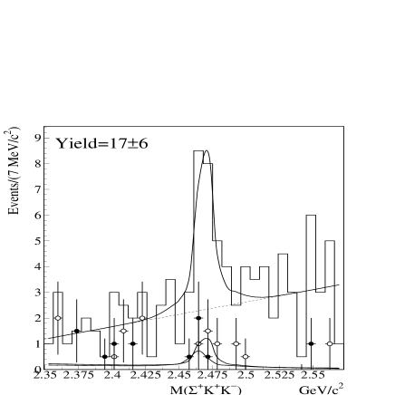
Figure 4: The histogram shows the inclusive $\Sigma^{+}(p\pi^{0})K^{+}K^{-}$ invariant mass distribution, the data is fit to two Gaussians for the signal and a first order polynomial for the background. The points with error bars show the possible contribution from $\Sigma^{+}\phi$ (empty circles) and $\Xi^{*}(1690)^{0}K^{+}$ (filled circles).

The $\Sigma^{+}K^{+}K^{-}$ invariant mass distribution is shown in Fig. 4. The fit is performed using a double Gaussian for the signal and a first order polynomial for the background. Again, the ratio of yields, the resolutions of the two Gaussians and the mean of the wide Gaussian are fixed to the Monte Carlo values. The fit returns $17\pm 6$ events. The branching ratio relative to $\Xi_{c}^{+}\rightarrow\Sigma^{+}K^{-}\pi^{+}$ is

$$\frac{\Gamma(\Xi_{c}^{+}\rightarrow\Sigma^{+}K^{+}K^{-})}{\Gamma(\Xi_{c}^{+}\rightarrow\Sigma^{+}K^{-}\pi^{+})}=0.16\pm 0.06~{}\textrm{(stat).}$$ (3)

As significant resonant structure is observed in the decay $\Lambda_{c}^{+}\rightarrow\Sigma^{+}K^{+}K^{-}$ [9, 10], we search for possible contribution from $\Xi_{c}^{+}\rightarrow\Sigma^{+}\phi$ and $\Xi_{c}^{+}\rightarrow\Xi^{*}(1690)^{0}K^{+}$. For both decays we fit the $\Sigma^{+}K^{+}K^{-}$ invariant mass distribution. For $\Xi_{c}^{+}\rightarrow\Sigma^{+}\phi$ decay we make a sideband subtraction on the $K^{+}K^{-}$ invariant mass (using $20~{}\textrm{MeV}/c^{2}$ wide signal region and sideband). For $\Xi_{c}^{+}\rightarrow\Xi^{*}(1690)^{0}K^{+}$ we require the $\Sigma^{+}K^{-}$ invariant mass to be within $20~{}\textrm{MeV}/c^{2}$ of the nominal $\Xi^{*}$ mass (where we assume no contribution from the non-resonant mode), and we exclude events in the $\phi$ signal region. No significant contribution is found. In Fig. 4 we show the fits of the two resonant modes superimposed to the inclusive sample. The fit reports $3\pm 2$ events for $\Sigma^{+}\phi$ and $2\pm 2$ for $\Xi^{*}(1690)^{0}K^{+}$. We set the upper limit at 90% confidence level for the branching fractions relative to $\Xi_{c}^{+}\rightarrow\Sigma^{+}K^{-}\pi^{+}$ to be

$$\frac{\Gamma(\Xi_{c}^{+}\rightarrow\Sigma^{+}\phi)}{\Gamma(\Xi_{c}^{+}\rightarrow\Sigma^{+}K^{-}\pi^{+})}<0.12$$ (4)

and

$$\frac{\Gamma(\Xi_{c}^{+}\rightarrow\Xi(1690)^{0}K^{+})}{\Gamma(\Xi_{c}^{+}\rightarrow\Sigma^{+}K^{-}\pi^{+})}<0.05,$$ (5)

where no correction is made for the branching ratio of $\Xi^{*}(1690)^{0}\rightarrow\Sigma^{+}K^{-}$. For both modes we find a negligible systematic uncertainty.

4 $\Xi_{c}^{+}\rightarrow\Lambda^{0}K^{-}\pi^{+}\pi^{+}$, $\Xi_{c}^{+}\rightarrow\Omega^{-}K^{+}\pi^{+}$ and $\Xi_{c}^{+}\rightarrow\Sigma^{*}(1385)^{+}\bar{K}^{0}$ decays

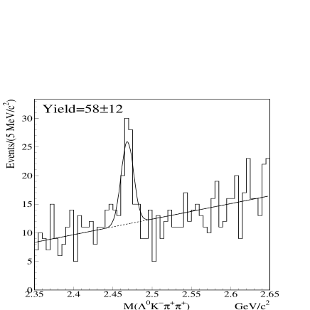
Figure 5: Invariant mass distribution for $\Lambda^{0}K^{-}\pi^{+}\pi^{+}$. The fit function is a sum of a Gaussian for the signal and a linear background.

We measure the branching ratio of the decay $\Xi_{c}^{+}\rightarrow\Lambda^{0}K^{-}\pi^{+}\pi^{+}$ relative to $\Xi_{c}^{+}\rightarrow\Xi^{-}\pi^{+}\pi^{+}$. The sample is selected requiring a significance of separation ($L/\sigma_{L}$) greater than $5$, $\mathrm{CLD}>2\%$, and $\sigma_{t}<100$ fs. Furthermore, the kaon hypothesis must be favored over the pion hypothesis ($W(\pi)-W(K)>2$), while the pion must satisfy $\min\{W_{\alpha}\}-W_{\pi}>-6$. The invariant mass distribution for $\Lambda^{0}K^{-}\pi^{+}\pi^{+}$ is shown in Fig. 5. The fit is performed using a Gaussian for the signal plus a linear polynomial for the background. The signal yield is $58\pm 12$ events. The same selection cuts are applied to the normalization mode $\Xi_{c}^{+}\rightarrow\Xi^{-}\pi^{+}\pi^{+}$ to minimize possible systematic biases. We find the branching ratio of $\Xi_{c}^{+}\rightarrow\Lambda^{0}K^{-}\pi^{+}\pi^{+}$ relative to $\Xi_{c}^{+}\rightarrow\Xi^{-}\pi^{+}\pi^{+}$ to be

$$\frac{\Gamma(\Xi_{c}^{+}\rightarrow\Lambda^{0}K^{-}\pi^{+}\pi^{+})}{\Gamma(\Xi_{c}^{+}\rightarrow\Xi^{-}\pi^{+}\pi^{+})}=0.28\pm 0.06~{}\textrm{(stat)}.$$ (6)

We find an indication of the decay $\Xi_{c}^{+}\rightarrow\Omega^{-}K^{+}\pi^{+}$. The sample is selected by reconstructing the $\Omega^{-}$ when it decays to $\Lambda^{0}K^{-}$. The $\Lambda^{0}K^{-}$ invariant mass must be within $20~{}\textrm{MeV}/c^{2}$ of the nominal $\Omega^{-}$ mass and the decay vertex must satisfy a minimum confidence level cut of $1\%$. The significance of separation, $L/\sigma_{L}$, must be greater than 0.5. The kaon from the decay vertex must be favored with respect to the pion hypothesis ($W(\pi)-W(K)>2$), while the pion must satisfy $\min\{W_{\alpha}\}-W_{\pi}>-6$.

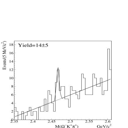
Figure 6: Invariant mass distribution for the combination $\Omega^{-}K^{+}\pi^{+}$. The fit is performed using a single Gaussian for the signal plus a first order polynomial for the background.

The $\Omega^{-}K^{+}\pi^{+}$ invariant mass distribution is shown in Fig. 6. The data is fit with a single Gaussian for the signal and a linear polynomial for the background. We used similar cuts for the normalization mode. We report the value, for the branching ratio of $\Xi_{c}^{+}\rightarrow\Omega^{-}K^{+}\pi^{+}$ relative to $\Xi_{c}^{+}\rightarrow\Xi^{-}\pi^{+}\pi^{+}$, to be

$$\frac{\Gamma(\Xi_{c}^{+}\rightarrow\Omega^{-}K^{+}\pi^{+})}{\Gamma(\Xi_{c}^{+}\rightarrow\Xi^{-}\pi^{+}\pi^{+})}=0.07\pm 0.03~{}\textrm{(stat)}.$$ (7)

After evaluation of the systematic uncertainty as described in the last section, we measure the upper limit at 90% confidence level to be

$$\frac{\Gamma(\Xi_{c}^{+}\rightarrow\Omega^{-}K^{+}\pi^{+})}{\Gamma(\Xi_{c}^{+}\rightarrow\Xi^{-}\pi^{+}\pi^{+})}<0.12.$$ (8)

We also see an indication of the decay $\Xi_{c}^{+}\rightarrow\Sigma^{*}(1385)^{+}\bar{K}^{0}$ where the $\Sigma^{*}$ is reconstructed in the decay mode $\Lambda^{0}$$\pi^{+}$. The invariant mass of this combination is required to be in the interval $1.349$–$1.421~{}\textrm{GeV}/c^{2}$ which corresponds to a $\pm 1.0~{}\Gamma$ window around the $\Sigma^{*}$ nominal mass. The $\bar{K}^{0}$ is reconstructed as a $K_{S}^{0}$ in the $\pi^{+}$$\pi^{-}$ decay mode. We require that the reconstructed invariant mass of the $\pi^{+}\pi^{-}$ lie within 3 standard deviations of the nominal $K^{0}_{S}$ mass. We select the events by requiring $\mathrm{CLD}>3\%$ and the significance of detachment $L/\sigma_{L}$ greater than 4.5. We also reject events where the $\pi^{+}$ track from the decay vertex has a confidence level greater than 0.1% of coming from the production vertex. Further, the $\Xi_{c}^{+}$ candidates must have a momentum greater than $45~{}\textrm{GeV}/c$. We identify the pion from the $\Sigma^{*}$ by requiring $\min\{W_{\alpha}\}-W_{\pi}>-6$.

Figure 7: Invariant mass of the $\Lambda^{0}\pi^{+}K_{S}^{0}$ combination for the $\Xi_{c}^{+}\rightarrow\Sigma^{*}(1385)^{+}\bar{K}^{0}$ decay mode. The fit is to a Gaussian for the signal events and a first order polynomial for the background.

In Fig.7 the $\Lambda^{0}\pi^{+}K_{S}^{0}$ invariant mass is shown. We measure the branching ratio relative to $\Xi_{c}^{+}\rightarrow\Xi^{-}\pi^{+}\pi^{+}$ to be

$$\frac{\Gamma(\Xi_{c}^{+}\rightarrow\Sigma^{*}(1385)^{+}\bar{K}^{0})}{\Gamma(\Xi_{c}^{+}\rightarrow\Xi^{-}\pi^{+}\pi^{+})}=1.00\pm 0.49~{}\textrm{(stat)}.$$ (9)

We find the upper limit for the branching ratio at 90% confidence level to be

$$\frac{\Gamma(\Xi_{c}^{+}\rightarrow\Sigma^{*}(1385)^{+}\bar{K}^{0})}{\Gamma(\Xi_{c}^{+}\rightarrow\Xi^{-}\pi^{+}\pi^{+})}<1.72;$$ (10)

this measurement includes the systematic uncertainty.

5 Search for the resonant decay $\Xi_{c}^{+}\rightarrow\Xi^{*}(1530)^{0}\pi^{+}$

As most of the branching ratios are computed relative to $\Xi_{c}^{+}\rightarrow\Xi^{-}\pi^{+}\pi^{+}$, we investigate possible systematic errors due to a contribution from $\Xi_{c}^{+}\rightarrow\Xi^{*}(1530)^{0}\pi^{+}$. The decay width of this mode is expected to be zero [1]. In Fig. 8 we plot the sideband subtracted invariant mass distribution for the two possible combinations of $\Xi^{-}\pi^{+}$ in the $\Xi^{-}\pi^{+}\pi^{+}$ sample. We fit the signal events using a Breit-Wigner. The background is given by two contributions, the non-resonant $\Xi_{c}^{+}\rightarrow\Xi^{-}\pi^{+}\pi^{+}$ events and the wrong $\Xi^{-}\pi^{+}$ combination. Both shapes for these distributions are obtained from a Monte Carlo simulation. The width and mean of the Breit-Wigner and the ratio between the Breit-Wigner amplitude and the amplitude of the wrong sign combination, are fixed to the Monte Carlo values. No significant contribution from this resonant structure is found. After evaluation of the systematic uncertainty, we find the upper limit at $90\%$ confidence level for the branching ratio relative to $\Xi_{c}^{+}\rightarrow\Xi^{-}\pi^{+}\pi^{+}$ to be

$$\frac{\Gamma(\Xi_{c}^{+}\rightarrow\Xi^{*}(1530)^{0}\pi^{+})}{\Gamma(\Xi_{c}^{+}\rightarrow\Xi^{-}\pi^{+}\pi^{+})}<0.10.$$ (11)

Figure 8: A fit to the $\Xi^{-}\pi^{+}$ sideband-subtracted invariant mass distribution performed using a Breit-Wigner for the signal region plus a shape for the non-resonant $\Xi_{c}^{+}\rightarrow\Xi^{-}\pi^{+}\pi^{+}$ and the wrong ($\Xi^{-}$$\pi^{+}$) combinations taken by Monte Carlo simulation. The Breit-Wigner width and mean are fixed to the Monte Carlo values.

We calculate that in the case of a contamination from the resonant substructure up to a level of 10%, the efficiency of $\Xi^{-}\pi^{+}\pi^{+}$ inclusive would change by less than 1%. For this reason the $\Xi^{-}\pi^{+}\pi^{+}$ efficiencies for the branching ratio measurements have been evaluated with a non-resonant Monte Carlo.

6 Systematic studies

The systematic uncertainties are evaluated after investigation of two possible sources: the choice of fitting conditions and the Monte Carlo simulation. The total systematic error is computed by adding in quadrature these two independent contributions. We measure the systematic uncertainty due to fitting conditions using a fit variation technique, which includes variations in bin size, fitting range, background shapes, sidebands size and position. To assess possible systematic uncertainties related to the Monte Carlo simulation we used the standard FOCUS split sample technique, described in [11], and based on the S-factor method used by the Particle Data Group [12]. We investigate possible biases due to poor simulation of variables such as run period, particle and antiparticle, $\Sigma^{+}$ decay mode and momentum, $\Xi_{c}^{+}$ momentum and significance of separation between production and decay vertices. Furthermore, as noted above, we find that the efficiency of the $\Xi^{-}\pi^{+}\pi^{+}$ mode is not affected by possible resonant structure. Due to the low statistics, no split sample studies are made for $\Xi_{c}^{+}\rightarrow\Sigma^{+}K^{+}K^{-}$, $\Xi_{c}^{+}\rightarrow\Sigma^{+}\phi$, $\Xi_{c}^{+}\rightarrow\Xi^{*}(1690)^{0}K^{+}$, $\Xi_{c}^{+}\rightarrow\Xi^{*}(1530)^{-}\pi^{+}$ and $\Xi_{c}^{+}\rightarrow\Sigma^{*}(1385)^{+}\bar{K}^{0}$. Because of the particular spin properties of the particles involved in the latter decay mode, we evaluated a possible systematic uncertainty of our simulation by varying the Monte Carlo angular distribution to match the shape obtained in the data. In Table 1 we summarize the systematic uncertainty for each mode. In Table 2 we present the FOCUS results with a comparison to previous measurements from CLEO [13] and SELEX [14].

Table 1: The systematic uncertainties from the Monte Carlo simulation, the fitting condition, and total for each mode are shown.

Systematic Error

Mode	Simulation	Fit	Total
$\frac{\Gamma(\Xi_{c}^{+}\!~{}\rightarrow~{}\!\Sigma^{+}K^{-}\pi^{+})}{\Gamma(\Xi_{c}^{+}\!~{}\rightarrow~{}\!\Xi^{-}\pi^{+}\pi^{+})}$	0.00	0.04	0.04
$\frac{\Gamma(\Xi_{c}^{+}\!~{}\rightarrow~{}\!\Sigma^{+}\bar{K}^{*}(892)^{0})}{\Gamma(\Xi_{c}^{+}\!~{}\rightarrow~{}\!\Xi^{-}\pi^{+}\pi^{+})}$	0.00	0.06	0.06
$\frac{\Gamma(\Xi_{c}^{+}\!~{}\rightarrow~{}\!\Sigma^{+}K^{+}K^{-})}{\Gamma(\Xi_{c}^{+}\!~{}\rightarrow~{}\!\Sigma^{+}K^{-}\pi^{+})}$	—	0.01	0.01
$\frac{\Gamma(\Xi_{c}^{+}\!~{}\rightarrow~{}\!\Lambda^{0}K^{-}\pi^{+}\pi^{+})}{\Gamma(\Xi_{c}^{+}\!~{}\rightarrow~{}\!\Xi^{-}\pi^{+}\pi^{+})}$	0.05	0.04	0.06
$\frac{\Gamma(\Xi_{c}^{+}\!~{}\rightarrow~{}\!\Omega^{-}K^{+}\pi^{+})}{\Gamma(\Xi_{c}^{+}\!~{}\rightarrow~{}\!\Xi^{-}\pi^{+}\pi^{+})}$	0.03	0.01	0.03
$\frac{\Gamma(\Xi_{c}^{+}\!~{}\rightarrow~{}\!\Sigma^{*}(1385)^{+}\bar{K}^{0})}{\Gamma(\Xi_{c}^{+}\!~{}\rightarrow~{}\!\Xi^{-}\pi^{+}\pi^{+})}$	0.19	0.14	0.24

Table 2: FOCUS results compared to previous measurements. The relative efficiencies are computed with respect to the normalization mode (for $\Xi_{c}^{+}\rightarrow\Xi^{*}(1690)^{0}K^{+}$ we do not correct for the branching fraction of $\Xi^{*}(1690)^{0}\rightarrow\Sigma^{+}K^{-}$ as it is not known).

Relative Branching Ratio

Decay Mode	Efficiency Ratio	FOCUS	CLEO	SELEX
$\frac{\Gamma(\Xi_{c}^{+}\!~{}\rightarrow~{}\!\Sigma^{+}K^{-}\pi^{+})}{\Gamma(\Xi_{c}^{+}\!~{}\rightarrow~{}\!\Xi^{-}\pi^{+}\pi^{+})}$	1.04	$0.91\pm 0.11\pm 0.04$	$1.18\pm 0.26\pm 0.17$	$0.92\pm 0.20\pm 0.07$
$\frac{\Gamma(\Xi_{c}^{+}\!~{}\rightarrow~{}\!\Sigma^{+}\bar{K}^{*}(892)^{0})}{\Gamma(\Xi_{c}^{+}\!~{}\rightarrow~{}\!\Xi^{-}\pi^{+}\pi^{+})}$	0.57	$0.78\pm 0.16\pm 0.06$	$0.92\pm 0.27\pm 0.17$	—
$\frac{\Gamma(\Xi_{c}^{+}\!~{}\rightarrow~{}\!\Sigma^{+}K^{+}K^{-})}{\Gamma(\Xi_{c}^{+}\!~{}\rightarrow~{}\!\Sigma^{+}K^{-}\pi^{+})}$	0.77	$0.16\pm 0.06\pm 0.01$	—	—
$\frac{\Gamma(\Xi_{c}^{+}\!~{}\rightarrow~{}\!\Sigma^{+}\phi)}{\Gamma(\Xi_{c}^{+}\!~{}\rightarrow~{}\!\Sigma^{+}K^{-}\pi^{+})}$	0.33	$<0.12$ at 90$\%$ C.L.	—	—
$\frac{\Gamma(\Xi_{c}^{+}\!~{}\rightarrow~{}\!\Xi^{*}(1690)^{0}K^{+})}{\Gamma(\Xi_{c}^{+}\!~{}\rightarrow~{}\!\Sigma^{+}K^{-}\pi^{+})}$	0.57	$<0.05$ at 90$\%$ C.L.	—	—
$\frac{\Gamma(\Xi_{c}^{+}\!~{}\rightarrow~{}\!\Lambda^{0}K^{-}\pi^{+}\pi^{+})}{\Gamma(\Xi_{c}^{+}\!~{}\rightarrow~{}\!\Xi^{-}\pi^{+}\pi^{+})}$	1.09	$0.28\pm 0.06\pm 0.06$	$0.58\pm 0.16\pm 0.07$	—
$\frac{\Gamma(\Xi_{c}^{+}\!~{}\rightarrow~{}\!\Omega^{-}K^{+}\pi^{+})}{\Gamma(\Xi_{c}^{+}\!~{}\rightarrow~{}\!\Xi^{-}\pi^{+}\pi^{+})}$	1.40	$0.07\pm 0.03\pm 0.03$	—	—
		$<0.12$ at 90$\%$ C.L.
$\frac{\Gamma(\Xi_{c}^{+}\!~{}\rightarrow~{}\!\Sigma^{*}(1385)^{+}\bar{K}^{0})}{\Gamma(\Xi_{c}^{+}\!~{}\rightarrow~{}\!\Xi^{-}\pi^{+}\pi^{+})}$	0.21	$1.00\pm 0.49\pm 0.24$	—	—
		$<1.72$ at 90$\%$ C.L.
$\frac{\Gamma(\Xi_{c}^{+}\!~{}\rightarrow~{}\!\Xi^{*}(1530)^{0}\pi^{+})}{\Gamma(\Xi_{c}^{+}\!~{}\rightarrow~{}\!\Xi^{-}\pi^{+}\pi^{+})}$	0.62	$<0.10$ at 90$\%$ C.L.	$<0.2$ at 90$\%$ C.L	—

7 Conclusions

We investigate and measure the relative branching ratios of several decay modes of the charm baryon $\Xi_{c}^{+}$. We report the first evidence for the Cabibbo suppressed decay $\Xi_{c}^{+}\rightarrow\Sigma^{+}K^{+}K^{-}$ and we investigate the contribution from the resonant modes $\Xi_{c}^{+}\rightarrow\Sigma^{+}\phi$ and $\Xi_{c}^{+}\rightarrow\Xi^{*}(1690)^{0}K^{+}$. We report an indication of the decays $\Xi_{c}^{+}\rightarrow\Omega^{-}K^{+}\pi^{+}$ and $\Xi_{c}^{+}\rightarrow\Sigma^{*}(1385)\bar{K}^{0}$. We also report improved measurements of $\Xi_{c}^{+}$ decays in the final state $\Sigma^{+}K^{-}\pi^{+}$, $\Sigma^{+}\bar{K}^{*}(892)^{0}$ and $\Lambda^{0}K^{-}\pi^{+}\pi^{+}$. These last three results agree with previous measurements from the the CLEO and SELEX collaborations. Finally, we report an improved measurement of the limit for the resonant decay $\Xi_{c}^{+}\rightarrow\Xi^{*}(1530)^{0}\pi^{+}$.

8 Acknowledgements

We wish to acknowledge the assistance of the staffs of Fermi National Accelerator Laboratory, the INFN of Italy, and the physics departments of the collaborating institutions. This research was supported in part by the U. S. National Science Foundation, the U. S. Department of Energy, the Italian Istituto Nazionale di Fisica Nucleare and Ministero dell’Università e della Ricerca Scientifica e Tecnologica, the Brazilian Conselho Nacional de Desenvolvimento Científico e Tecnológico, CONACyT-México, the Korean Ministry of Education, and the Korean Science and Engineering Foundation.

References

[1]
J. G. Körner and
M. Krämer,
Z. Phys.
C 55 (1992) 659.
[2]
F. Hussain,
J. G. Körner,
M. Krämer, and
G. Thompson,
Z. Phys.
C 51 (1991) 321.
[3]
B. Guberina and
H. Stefancic,
Phys. Rev.
D 65 (2002) 114004.
[4]
J. M. Link et al.
(FOCUS), Phys. Lett.
B 523 (2001) 53.
[5]
J. M. Link et al.
(FOCUS) (2002),
submitted to Nucl. Instrum. Methods A, hep-ex/0204023.
[6]
J. M. Link et al.
(FOCUS), Nucl. Instrum. Methods
A 484 (2002) 174.
[7]
P. L. Frabetti et al.
(E687), Nucl. Instrum. Methods
A 320 (1992) 519.
[8]
J. M. Link et al.
(FOCUS), Nucl. Instrum. Methods
A 484 (2002) 270.
[9]
J. M. Link et al.
(FOCUS), Phys. Lett.
B 540 (2002) 25.
[10]
K. Abe et al.
(BELLE), Phys. Lett.
B 524 (2002) 33.
[11]
J. M. Link et al.
(FOCUS), Phys. Lett.
B 555 (2003) 167.
[12]
D. E. Groom et al.,
Particle Data Group, Eur. Phys. J. C.
15 (2000) 1.
[13]
T. Bergfeld et al.
(CLEO), Phys. Lett.
B 365 (1996) 431.
[14]
S. Y. Jun et al.
(SELEX), Phys. Rev. Lett.
84 (2000) 1857.