Study of the $q^{2}$–dependence of $B\to\pi\ell\nu$ and $B\to\rho(\omega)\ell\nu$ Decay and Extraction of $|V_{ub}|$

Abstract

We report on determinations of $|V_{ub}|$ resulting from studies of the branching fraction and $q^{2}$ distributions in exclusive semileptonic $B$ decays that proceed via the $b\to u$ transition. Our data set consists of the $9.7\times 10^{6}$ $B\overline{B}$ meson pairs collected at the $\Upsilon(4S)$ resonance with the CLEO II detector. We measure ${\cal B}(B^{0}\to\pi^{-}\ell^{+}\nu)=(1.33\pm 0.18\pm 0.11\pm 0.01\pm 0.07)\times 10^{-4}$ and ${\cal B}(B^{0}\to\rho^{-}\ell^{+}\nu)=(2.17\pm 0.34\;^{+0.47}_{-0.54}\pm 0.41\pm 0.01)\times 10^{-4}$, where the errors are statistical, experimental systematic, systematic due to residual form–factor uncertainties in the signal, and systematic due to residual form–factor uncertainties in the cross–feed modes, respectively. We also find ${\cal B}(B^{+}\to\eta\ell^{+}\nu)=(0.84\pm 0.31\pm 0.16\pm 0.09)\times 10^{-4}$, consistent with what is expected from the $B\to\pi\ell\nu$ mode and quark model symmetries. We extract $|V_{ub}|$ using Light-Cone Sum Rules (LCSR) for $0\leq q^{2}<16$ GeV² and Lattice QCD (LQCD) for 16 GeV² $\leq q^{2}<q^{2}_{\rm max}$. Combining both intervals yields $|V_{ub}|=(3.24\pm 0.22\pm 0.13\;^{+0.55}_{-0.39}\pm 0.09)\times 10^{-3}$ for $\pi\ell\nu$, and $|V_{ub}|=(3.00\pm 0.21\;^{+0.29}_{-0.35}\;{}^{+0.49}_{-0.38}\pm 0.28)\times 10^{-3}$ for $\rho\ell\nu$, where the errors are statistical, experimental systematic, theoretical, and signal form-factor shape, respectively. Our combined value from both decay modes is $|V_{ub}|=(3.17\pm 0.17\;^{+0.16}_{-0.17}\;{}^{+0.53}_{-0.39}\pm 0.03)\times 10^{-3}$.

I Introduction

The element $V_{ub}$ remains one of the most poorly constrained parameters of the Cabbibo-Kobayashi-Maskawa (CKM) matrix bb:CKM . Its magnitude, $|V_{ub}|$, plays a central role in constraints based on the unitarity of the CKM matrix and inputs from both $CP$–conserving processes in the $B$ meson decay and $CP$–violating processes in the neutral kaon and $B$ systems. The value of $|V_{ub}|$ and, in particular, the accuracy to which we have measured this important parameter, have been the subjects of considerable debate over the past decade bb:PDG_vub_minireview . An accurate determination of $|V_{ub}|$ with well-understood uncertainties remains one of the fundamental priorities for heavy flavor physics.

A number of $|V_{ub}|$ measurement approaches have been attempted, and are reviewed in reference bb:PDG_vub_minireview . Inclusive techniques are hampered by a mismatch in kinematic regions where the large experimental backgrounds from $b\to c\ell\nu$ can be suppressed versus regions in which the theoretical uncertainties can be reliably determined. For exclusive reconstruction of particular final states, the primary challenge is calculation of the form factors for those channels. The first measurements of exclusive charmless semileptonic branching fractions bb:lkg_cleo_exclusive , including evaluation of $|V_{ub}|$, were performed by the CLEO experiment at the Cornell Electron Storage Ring (CESR) using the modes $B^{0}\to\pi^{-}\ell^{+}\nu$, $B^{+}\to\pi^{0}\ell^{+}\nu$, $B^{0}\to\rho^{-}\ell^{+}\nu$, $B^{+}\to\rho^{0}\ell^{+}\nu$, $B^{+}\to\omega\ell^{+}\nu$, and charge-conjugate decays, where $\ell=e\text{ or }\mu$. A second measurement of the $\rho\ell\nu$ modes by CLEO bb:lange_cleo_exclusive , using similar techniques but a much different signal to background optimization, provided consistent, essentially independent, results with a similar total uncertainty. The combined analyses yielded $|V_{ub}|=(3.25\pm 0.14^{+0.21}_{-0.29}\pm 0.55)\times 10^{-3}$, where the errors are statistical, experimental systematic and estimated theoretical uncertainties, respectively. The $\pi$ and $\rho$ modes contribute about equally to this result.

This paper presents an update of the original exclusive $B\to X_{u}\ell\nu$ analysis bb:lkg_cleo_exclusive , and is based on a total data sample of $9.7\times 10^{6}$ $B\bar{B}$ pairs collected on the $\Upsilon(4S)$ resonance. The results presented here supersede those of reference bb:lkg_cleo_exclusive . In addition to using a larger data set, the analysis has been modified to minimize uncertainties arising from the momentum-transfer ($q^{2}$) dependence of the form factors. Most notably, the lower bounds on the charged-lepton momentum for both the pseudoscalar and the vector modes have been lowered, and the branching fractions are determined independently in three $q^{2}$ regions. For the $\rho$ modes, the branching fractions as a function of $q^{2}$ were first determined by the second CLEO $\rho\ell\nu$ analysis bb:lange_cleo_exclusive . The present analysis has a significantly broader accepted range for the charged lepton momentum, which allows for better discrimination among models. A detailed description of this analysis can be found in reference bb:vb_thesis .

II Exclusive charmless semileptonic decays

The semileptonic transition of a $B$ meson (a pseudoscalar) to a final state with a single pseudoscalar meson $P$ can, in the limit of a massless charged lepton, be described by a single form factor $f_{1}(q^{2})$:

$$\frac{d\Gamma(B^{0}\to P^{-}\ell^{+}\nu)}{dy\,d\cos\theta_{W\ell}}=|V_{ub}|^{2}\frac{G_{F}^{2}k_{P}^{3}M_{B}^{2}}{32\pi^{3}}\sin^{2}\theta_{W\ell}|f_{1}(q^{2})|^{2},$$ (1)

where $y=q^{2}/M_{B}^{2}$, $M_{B}$ is the mass of the $B$ meson, $G_{F}$ is the Fermi constant, $k_{P}$ is the meson momentum, and $\theta_{W\ell}$ is the angle between the charged lepton direction in the virtual $W$ ($\ell+\nu$) rest frame and the direction of the virtual $W$ in the $B$ rest frame. For a transition to a final state with a single vector meson $V$, three form factors ($A_{1}$, $A_{2}$, and $V$) are necessary:

$$\frac{d\Gamma(B^{0}\to V^{-}\ell^{+}\nu)}{dy\,d\cos\theta_{W\ell}} = |V_{ub}|^{2}\frac{G_{F}^{2}k_{V}M_{B}^{2}y}{128\pi^{3}}\times$$

$$\left[(1-\cos\theta_{W\ell})^{2}\frac{|H_{+}|^{2}}{2}+(1+\cos\theta_{W\ell})^{2}\frac{|H_{-}|^{2}}{2}+\sin^{2}\theta_{W\ell}|H_{0}|^{2}\right],$$

where $k_{V}$ is the meson momentum and the three helicity amplitudes are given by

$$H_{\pm} = \frac{1}{M_{B}+m_{V}}\left[A_{1}(q^{2})\mp 2M_{B}k_{V}V(q^{2})\right]\ ,\ \ {\rm and}$$ (3)

$$H_{0} = \frac{1}{\sqrt{y}}\frac{M_{B}}{2m_{V}(M_{B}+m_{V})}\left[\left(1-\frac{m_{V}^{2}}{M_{B}^{2}}-y\right)A_{1}(q^{2})-4k_{V}^{2}A_{2}(q^{2})\right].$$ (4)

The structure of these differential decay rates immediately allows us to draw some general conclusions regarding the properties of the semileptonic decays that we reconstruct in this analysis. For the $\rho(\omega)\ell\nu$ transitions, the left-handed, $V-A$, nature of the charged current at the quark level manifests itself at the hadronic level as $|H_{-}|>|H_{+}|$. The $H_{-}$ contribution is also expected to dominate the $H_{0}$ contribution, leading to a forward-peaked distribution for $\cos\theta_{W\ell}$. For $\pi(\eta)\ell\nu$, there is a $\sin^{2}\theta_{W\ell}$ dependence, independent of the form factor. The pseudoscalar modes also contain an extra factor of the meson momentum squared, which suppresses the rate near $q^{2}_{\text{max}}$ ($k_{P}=0$). Taken together, these two effects give the pseudoscalar modes a softer charged lepton momentum spectrum than the vector modes.

Calculation of the form factors has become a considerable theoretical industry, with a variety of techniques now being employed. Form factors based on lattice QCD (LQCD) calculations Abada:1993dh ; Allton:1994ui ; DelDebbio:1997kr ; Hashimoto:1997sr ; Ryan:1998tj ; Ryan:1999kx ; Lellouch:1999dz ; Bowler:1999xn ; Becirevic:1999kt ; Aoki:2000by ; El-Khadra:2001rv ; Aoki:2001rd ; Abada:2000ty and on light-cone sum rules (LCSR) Ball:1997rj ; Ball:1998kk ; Khodjamirian:1997ub ; Khodjamirian:2000ds ; Bakulev:2000fb ; Huang:2000hs ; Wang:2001mi ; Wang:2001bh ; Ball:2001fp currently have uncertainties in the $15\%$ to $20\%$ range. A variety of quark-model calculations exist Wirbel:1985ji ; Korner:1987kd ; Isgur:gb ; Scora:1995ty ; Melikhov:1995xz ; Beyer:1998ka ; Faustov:1995bf ; Demchuk:1997uz ; Grach:1996nz ; :2000ae ; Melikhov:2000yu ; Feldmann:1999sm ; Flynn:2000gd ; Beneke:2000wa ; Choi:1999nu . Finally, a number of other approaches Kurimoto:2001zj ; Ligeti:1995yz ; Aitala:1997cm ; Burdman:1996kr ; Lellouch:1995yv ; Mannel:1998kp , such as dispersive bounds and experimentally–constrained models based on heavy quark symmetry, all seek to improve the range of $q^{2}$ over which the form factors can be estimated without introduction of significant model dependence. Figure 1 illustrates the broad variation in shape that arises in the literature. Unfortunately, all the form-factor calculations currently have contributions to the uncertainty that are uncontrolled. The light-cone sum rules calculations assume quark–hadron duality, offering a “canonical” contribution to the uncertainty of $10\%$, but with no known means of rigorously estimating that uncertainty. The LQCD calculations to date remain in the “quenched” approximation (no light quark loops in the propagators), which limits the ultimate precision to the 15% to 20% range. With the quark-model calculations it is difficult to quantify the uncertainty of a particular calculation by their very nature. These uncertainties in the form factors translate directly into the same fractional uncertainty on $|V_{ub}|$.

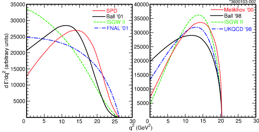
Figure 1: Predictions for $d\Gamma(B\to\pi\ell\nu)/dq^{2}$ (left) and for $d\Gamma(B\to\rho\ell\nu)/dq^{2}$ (right) for a variety of calculations, illustrating the range of variation of the predicted $q^{2}$–dependence. See Section VI for further discussion of the calculations.

In the $\pi\ell\nu$ modes, with only a single form factor in the massless lepton approximation, we expect that the rates extracted in the $q^{2}$ intervals that we have chosen will be largely independent of the form-factor shapes. In the vector modes, however, the three form factors interfere and differences in this interference among models, particularly at lower $q^{2}$ values, can lead to a residual model dependence. To investigate this effect, we will analyze the vector modes with three separate charged lepton momentum requirements.

III Event reconstruction and selection

The CLEO detector bb:CLEO-nim ; bb:silicon-nim contains three concentric tracking devices within a 1.5 T superconducting solenoid that detect charged particles over 95% (93%) of the solid angle for the first third (last two thirds) of the data. For the last two thirds of the data, a silicon vertex detector replaced a straw-tube wire chamber. The momentum resolution at 2 GeV/$c$ is 0.6%. A CsI(Tl) electromagnetic calorimeter, also inside the solenoid, covers 98% of $4\pi$. A typical $\pi^{0}$ mass resolution is 6 MeV. Charged tracks are assigned the most probable mass based on specific ionization, time of flight, and the relative rates as a function of momentum for proton, $K^{+}$, and $\pi^{+}$ production in $B$ decay.

The undetected neutrino complicates analysis of semileptonic decays. Because of the good hermeticity of the CLEO detector, we can reconstruct the neutrino via the missing energy ($E_{\text{miss}}\equiv 2E_{\text{beam}}-\sum E_{i}$) and missing momentum ($\vec{P}_{\text{miss}}\equiv-\sum\vec{p}_{i}$) in each event. In the process $e^{+}e^{-}\to\Upsilon(4S)\to B\bar{B}$, the total energy of the beams is imparted to the $B\bar{B}$ system; at CESR, that system is at, or nearly at, rest. (A small crossing angle has been in use at CESR for most of the running.) The missing mass, $M^{2}_{\text{miss}}\equiv E^{2}_{\text{miss}}-|\vec{P}_{\text{miss}}|^{2}$, must be consistent, within resolution, with a massless neutrino. Specifically, we require $-0.5<M^{2}_{\text{miss}}/2E_{\text{miss}}<0.3\ \text{GeV}$ for events with a total charge $\Delta Q=0$, and $|M^{2}_{\text{miss}}|/2E_{\text{miss}}<0.3\ \text{GeV}$ for events with $|\Delta Q|=1$.

Signal Monte Carlo (MC) events show a $|\vec{P}_{\text{miss}}|$ resolution of 85 MeV/$c$. The resolution on $E_{\text{miss}}$ is about three times larger than the momentum resolution bb:emissres . Significant effort has been devoted to minimizing multiple counting of charged particles in the track reconstruction (e.g., particles that curl multiple times within the tracking volume), and to suppressing clusters in the calorimeter from charged hadrons that have interacted.

With an estimate of the neutrino four–momentum in hand, we can employ full reconstruction of our signal modes. Because the resolution on $E_{\text{miss}}$ is so much larger than that for $|\vec{P}_{\text{miss}}|$, we use $(E_{\nu},\vec{p}_{\nu})=(|\vec{P}_{\text{miss}}|,\vec{P}_{\text{miss}})$ for full reconstruction. The neutrino combined with the signal charged lepton ($\ell$) and meson ($m$) should satisfy, within resolution, the constraints on energy, $\Delta E\equiv(E_{\nu}+E_{\ell}+E_{m})-E_{\text{beam}}\approx 0$, and on momentum, $M_{m\ell\nu}\equiv[E_{\text{beam}}^{2}-|\alpha\vec{p}_{\nu}+\vec{p}_{\ell}+\vec{p}_{m}|^{2}]^{\frac{1}{2}}\approx M_{B}$, where $\alpha$ is chosen to force $\Delta E=0$. The neutrino momentum resolution dominates the $\Delta E$ resolution, so the momentum scaling corrects for the mismeasurement of the magnitude of the neutrino momentum in the $M_{m\ell\nu}$ calculation. Uncertainty in the neutrino direction then remains as the dominant source of smearing in this mass calculation.

We reconstruct $q^{2}=M_{W^{*}}^{2}=(p_{\nu}+p_{\ell})^{2}$ for each decay from the reconstructed charged lepton four–momentum and the missing momentum. In addition to using the scaled reconstructed momentum $\alpha\vec{p}$ described above, the direction of the missing momentum is changed through the smallest angle consistent with forcing $M_{m\ell\nu}=M_{B}$. This procedure results in a $q^{2}$ resolution of 0.3 GeV², independent of $q^{2}$. The $\pi\ell\nu$ and the $\rho\ell\nu$ modes are analyzed separately in the intervals $q^{2}<8$ GeV², $8\leq q^{2}<16$ GeV², and $q^{2}\geq 16$ GeV². For the $\omega\ell\nu$ and $\eta\ell\nu$ modes, for which we have low statistics, we sum over all $q^{2}$.

Information from specific ionization is combined with calorimetric and tracking measurements to identify electrons with $p_{\ell}>600\text{ MeV}/c$ over 90% of the solid angle. Particles registering hits in counters deeper than 5 interaction lengths over the polar angle range $|\cos\theta|<0.85$ are considered muons. Those with hits beyond 3 interaction lengths over $|\cos\theta|<0.71$ are used in a multiple-lepton veto, described below. Candidate leptons must have $p_{\ell}>1.0\text{ GeV}/c$ for the $\pi$ and $\eta$ (pseudoscalar) modes, and $p_{\ell}>1.5\text{ GeV}/c$ for the $\rho$ and $\omega$ (vector) modes, which can couple to the $W$ helicities $\pm 1$ and hence have a harder spectrum. This momentum requirement for the vector modes defines the nominal analysis. We also analyze the vector modes with the lepton momentum requirements $p_{\ell}>1.75\text{ GeV}/c$ and $p_{\ell}>2.0\text{ GeV}/c$. The identification efficiency above $1.5\text{ GeV}/c$ averages over 90%; the probability that a hadron is misidentified as an electron (muon), a fake lepton, is about 0.1% (1%).

The 5-interaction-length requirement for muons causes the muon acceptance to fall rapidly below 1.4 GeV/$c$. As a result, only electrons contribute at the low end of the momentum range we accept for $\pi\ell\nu$, and electrons dominate the measurement in the lowest $q^{2}$ interval.

A $\pi^{0}$ candidate must have a $\gamma\gamma$ mass within 2 standard deviations of the $\pi^{0}$ mass. We reconstruct the $\omega$ via its $\pi^{+}\pi^{-}\pi^{0}$ decay, reducing combinatoric background by rejecting combinations away from the center of the $\omega$ Dalitz plot. We reconstruct $\eta$ in both the $\gamma\gamma$ and the $\pi^{+}\pi^{-}\pi^{0}$ decay modes. For the $\gamma\gamma$, we require the reconstructed mass to be within 2 standard deviations of the $\eta$ mass (within about 26 MeV). For the $\pi^{+}\pi^{-}\pi^{0}$, we require $|m_{\pi^{+}\pi^{-}\pi^{0}}-m_{\eta}|<$ 10 MeV (about 1.7 times the resolution). We impose a kinematic mass constraint on the momentum of all $\pi^{0}$ or $\eta$ candidates in the $\gamma\gamma$ final state.

Backgrounds arise from the $e^{+}e^{-}\to q\bar{q}$ and $e^{+}e^{-}\to\tau^{+}\tau^{-}$ continuum, fake leptons, $b\to c\ell\nu$, and $B\to X_{u}\ell\nu$ modes other than the signal modes. Backgrounds from continuum processes are suppressed by use of two event-shape variables. The selection criteria were optimized using background and signal Monte Carlo samples, rather than data, to avoid potential bias. The first variable is the angle ($\cos\theta_{\mathrm{thrust}}$) between the thrust axis evaluated for the candidate signal–mode particles (not including the neutrino) and that for the rest of the event. (The thrust axes are signed by picking the hemisphere containing the most energy.) For $B\bar{B}$ events at CESR, the distribution in this variable is flat because the $B$’s are nearly at rest and thus their decay orientations are independent. For continuum events the distribution is strongly forward and backward peaked. The ratio $R_{2}$ of the second to the zeroth Fox-Wolfram moment bb:fox_wolfram , which distinguishes spherical from jetty topologies, is also utilized. The continuum background tends to have a small reconstructed $q^{2}$. We therefore tune the continuum cut employed in the $R_{2}$–$\cos\theta_{\mathrm{thrust}}$ plane separately in each $q^{2}$ interval, and separately for the $\pi$ and $\rho$ modes. Signal events with low $q^{2}$ appear rather jetty, so a cut using $R_{2}$, when data is binned over a broad $q^{2}$ range, would introduce an efficiency bias. So for the $\omega$ and $\eta$ modes, for which all $q^{2}$ regions are combined, only a $\cos\theta_{\mathrm{thrust}}$ cut is applied, reducing uncertainties from the $q^{2}$–dependence of the form factors. Our criteria suppress the continuum background by over a factor of 10 and are about 80% efficient.

The $|p_{\ell}|$ cuts greatly reduce background from $b\to c\to s\ell\nu$ and bias mildly against $b\to c\ell\nu$. For the vector modes, we further require $\cos\theta_{W\ell}>0$, since the signal rate is largely suppressed by $V-A$ outside this region, while the background is roughly flat in the region excluded, and falls off in the region accepted.

Backgrounds, particularly $b\to c\ell\nu$, can smear into the signal region in $\Delta E$ and $M_{m\ell\nu}$ when $\vec{P}_{\text{miss}}$ misrepresents $\vec{p}_{\nu}$. Such backgrounds are highly suppressed by rejecting events with multiple charged leptons or a total event charge $|\Delta Q|>1$, both of which indicate missing particles. Requiring $M^{2}_{\text{miss}}$ to be consistent with zero also provides powerful background suppression. Still, Monte Carlo studies show that the dominant remaining $b\to c\ell\nu$ events contain either a $K_{L}$ meson or a second neutrino (from $c\to s\ell\nu$, with the lepton not identified) that is roughly collinear with the primary neutrino.

Our selection criteria studies, based on statistical considerations, indicated that keeping the $|\Delta Q|=1$ sample as well as the $\Delta Q=0$ was favorable in spite of the poorer signal-to-background ratio. Further systematic considerations indicated that the use of the $|\Delta Q|=1$ sample remained advantageous for the pseudoscalar modes. For the vector, in particular the $\rho$ modes, however, the overall poorer signal-to-background ratio made the $|\Delta Q|=1$ sample overly sensitive to systematic effects in both the modelling of the $B\to X_{u}\ell\nu$ backgrounds and the simulation of the detector. Therefore for the vector modes we require $\Delta Q=0$.

IV Extraction of branching fractions

IV.1 Method and binning

To extract the branching fraction information, we performed a binned maximum likelihood fit that was extended to include the finite statistics of the Monte Carlo, off-resonance, and fake-lepton samples following the method of Barlow and Beeston bb:BarlowBeeston . The data in each mode were coarsely binned over the two dimensional region $5.175\leq M_{m\ell\nu}<5.2875\text{ GeV},|\Delta E|<0.75\text{ GeV}$. We further binned the data in the reconstructed $2\pi$ and $3\pi$ masses in the $\rho$ and $\omega$ modes. The $|\Delta Q|=1$ samples were binned separately from $\Delta Q=0$ samples. Separation of the net charge samples allowed us to take advantage of the better signal-to-noise ratio of the $|\Delta Q|=0$ sample while reducing our dependence on our knowledge of the absolute tracking efficiency. Finally, we binned the data in $q^{2}$ for the two $\pi\ell\nu$ and the two $\rho\ell\nu$ modes. For the $\omega\ell\nu$ and the $\eta\ell\nu$ modes, we combined all $q^{2}$ information into a single bin.

Our fitting strategy was designed to minimize dependence of the results on the details of the simulation – both from detector and physics standpoints. The choice of binning balanced separation of signal and background against reliance on detailed MC shape predictions. To help minimize the model dependence of the branching fraction determinations, we did not use information from the lepton momentum spectrum or from $\cos\theta_{W\ell}$ within the fit. Extraction of rates in the separate $q^{2}$ intervals further reduces reliance on the form factors.

The $\Delta E$ bin intervals used in the nominal fit were $-0.75\leq\Delta E<-0.45$ GeV, $-0.45\leq\Delta E<-0.15$ GeV, and $-0.15\leq\Delta E<0.25$ GeV (the $\Delta E$ signal band). The $M_{m\ell\nu}$ bin intervals were $5.175\leq M_{m\ell\nu}<5.2425\text{ GeV}$ and $5.2425\leq M_{m\ell\nu}<5.2875\text{ GeV}$. In the $\Delta E$ signal band, this second mass interval is divided into two equal bands. Hence we used a total of seven bins in these two variables. In the $\rho\ell\nu$ ($\omega\ell\nu$) modes, we used three equal bins over the 2$\pi$ ($3\pi$) mass range within $\pm 285$ MeV ($\pm 30$ MeV) of the nominal $\rho$ ($\omega$) mass. The three $q^{2}$ intervals in the $\pi\ell\nu$ and the $\rho\ell\nu$ modes were $q^{2}<8\ \mathrm{GeV}^{2}$, $8\leq q^{2}<16\ \mathrm{GeV}^{2}$, and $q^{2}\geq 16\ \mathrm{GeV}^{2}$. The number of bins for each mode in the nominal fit is summarized in Table 1. The nominal fit had a total of 259 bins. For studies in which the $|\Delta Q|=1$ sample is included in the $\rho$ and $\omega$ modes, the fit had an additional 147 bins for a total of 406 bins.

Table 1: Summary of the number of bins used in each mode for the nominal fit.

	$\Delta E$, $M_{m\ell\nu}$	$\Delta Q$	$M_{2\pi,3\pi}$	$q^{2}$	total
$\pi^{-}\ell^{+}\nu$	7	2	1	3	42
$\pi^{0}\ell^{+}\nu$	7	2	1	3	42
$\rho^{-}\ell^{+}\nu$	7	1	3	3	63
$\rho^{0}\ell^{+}\nu$	7	1	3	3	63
$\omega\ell^{+}\nu$	7	1	3	1	21
$\eta_{\gamma\gamma}\ell^{+}\nu$	7	2	1	1	14
$\eta_{3\pi}\ell^{+}\nu$	7	2	1	1	14

To examine yields, efficiency, and kinematics in this paper, we use the most sensitive bin (the “signal bin”) $5.265\leq M_{m\ell\nu}<5.2875\text{ GeV}$ and $-0.15\leq\Delta E<0.25\text{ GeV}$, though neighboring bins also contribute information to the fit. For comparison, the $M_{m\ell\nu}$ and $\Delta E$ resolutions are about 7 MeV and 100 MeV, respectively, dominated by the resolution on $|\vec{p}_{\nu}|$. The 2$\pi$ (or 3$\pi$) mass intervals $\pm 95$ MeV and $\pm 10$ MeV, centered on the nominal masses, are used for figures for $\rho$ and $\omega$ candidates, respectively.

To simplify the statistical interpretation of the results, we limited the number of multiple entries per event. For each individual mode, the candidate with the smallest $|\Delta E|$ among those satisfying $M_{m\ell\nu}>5.175$ GeV was chosen, independent of $q^{2}$. A given event could contribute to multiple modes, although contribution near the signal region in more than one mode was rare. In the $\rho$ and $\omega$ modes, each of the mass bins described above was considered a separate mode.

IV.2 Fit components and parameters

MC simulation provided the distributions in each mode for signal, the $b\to c$ background, the cross feed among the modes, and the feed down from higher mass $B\to X_{u}\ell\nu$ decays. It included a full description of the $b\to c$ and charm decay modes and a GEANT-based bb:GEANT detector model. The $X_{u}\ell\nu$ feed down was evaluated with a simulation of the $B\to X_{u}\ell\nu$ process based on an inclusive operator product expansion (OPE) calculation bb:inclusive_theory of $d\Gamma(B\to X_{u}\ell\nu)/dM_{X_{u}}$, using parameters determined from the CLEO analysis of the $B\to X_{s}\gamma$ photon spectrum bb:bsgamm_theor ; bb:bsgamm_exp (also used in the recent CLEO lepton-momentum end-point analysis bb:new_endpoint ). The nominal analysis combined this inclusive spectrum with the ISGW II model Scora:1995ty for all mesons through the $\rho(1450)$. For each exclusive mode, we “subtracted rate” from the inclusive calculation with a weight of the form $\exp{[-\alpha(M_{X_{u}}-M_{R})^{2}/\Lambda_{QCD}^{2}]}$, where $M_{R}$ is the central mass of the resonance $R$. At any given $M_{X_{u}}$, the rate remaining after this subtraction of the exclusive modes is hadronized nonresonantly. Variations of the inclusive parameters based on the uncertainties in the $B\to X_{s}\gamma$ analysis and variations of the hadronization model (e.g., fully nonresonant but with $\pi\pi\ell\nu$ removed from the $\rho$ mass region) are included in the systematic uncertainties. The signal modes are excluded from these $B\to X_{u}\ell\nu$ samples.

The contributions from events in which hadrons have faked the signal leptons and from continuum are evaluated using data. The electron and muon identification fake rates from pions, kaons, and protons are measured in data using a variety of tagged samples. The analysis is performed on a sample of hadronic events with no identified leptons, treating each track in turn as a signal electron and then a signal muon. The contribution in each mode is weighted according to the fake rate.

We determined the residual continuum background using data collected 60 MeV below the $\Upsilon$(4S) energy. The center-of-mass energy and cross–section differences were taken into account as necessary. For each combination of mode, reconstructed $q^{2}$ bin, and for each $\Delta Q$ value, we determined the rate over the full $\Delta E-M_{m\ell\nu}$ plane by applying all cuts, including continuum-suppression cuts, and then scaling according to the relative on–resonance and off–resonance luminosities. To smooth the statistical fluctuations within each combination, we determined the shape over the $\Delta E-M_{m\ell\nu}$ plane by the following procedure. First, we dropped the continuum-suppression cuts, and obtained the shape over the $\Delta E-M_{m\ell\nu}$ plane, for each combination from data. Then, from continuum $q\bar{q}$ MC, $\tau^{+}\tau^{-}$ MC, and our fake lepton samples, we determined the change in shape over the $\Delta E-M_{m\ell\nu}$ plane caused by application of the continuum-suppression cuts, i.e., we obtained the ratio of yields, with to without cuts, for each $\Delta E-M_{m\ell\nu}$ bin, for each combination. Applying the ratios so obtained to the off-resonance data without continuum-suppression cuts, we obtained the shape of the background over the $\Delta E-M_{m\ell\nu}$ plane, for each combination.

For each signal mode, we generated a sample of signal Monte Carlo that is flat in phase space and processed these samples with our GEANT-based detector simulation. As we analyze each reconstructed event, we reweight the event to correspond to a particular calculation for the form factors involved in the decay. This procedure allowed us to sample a variety of form factor calculations. For each mode, we determine the efficiency matrix for reconstructed versus true $q^{2}$. Given our resolution and binning, the matrix is essentially diagonal, as Table 2 shows for the $\pi\ell\nu$ form-factor calculation of Ball and Zwicky (Ball’01) Ball:2001fp .

Table 2: The efficiency matrix in percent describing the probability that an event from a given generated $q^{2}$ interval reconstructs in a given $q^{2}$ interval for $B^{0}\to\pi^{-}\ell^{+}\nu$ events that pass all cuts and reconstruct within the “signal region” of $\Delta E$ versus $M_{m\ell\nu}$. The efficiencies are based on Ball’01.

true $q^{2}$	reconstructed $q^{2}$
(GeV2)	0 – 8	8 – 16	$\geq 16$
0 – 8	2.5	0.07	0.001
8 – 16	0.07	4.6	0.06
$\geq 16$	0.000	0.15	4.4

For these results, we have examined the following form factors for the signal modes and cross–feed rates. For $\pi\ell\nu$: Ball and Zwicky (light-cone sum rules) Ball:2001fp , ISGW II (a nonrelativistic quark model) Scora:1995ty , and the skewed parton distributions (SPD) of Feldmann and Kroll Feldmann:1999sm . Other LQCD and LCSR calculations are also considered in extracting $|V_{ub}|$. For $\rho\ell\nu$: Ball and Braun (light-cone sum rules – Ball’98) Ball:1998kk , ISGW II, Melikhov and Stech (a relativistic quark model – Melikhov’00) Melikhov:2000yu , and UKQCD (a LQCD calculation – UKQCD 98) DelDebbio:1997kr . For $\eta\ell\nu$, we have only considered the ISGW II form factor. The above choices for $\pi\ell\nu$ and $\rho\ell\nu$ bracket the extremes in the variation of the shape of $d\Gamma/dq^{2}$ and hence provide a conservative estimate of the theoretical uncertainty on the branching fractions. In general, the theory references provide minimal guidance on the theoretical uncertainty in the form-factor shapes, and the variation among the chosen calculations appears larger than the variation expected within a given calculation. For nominal yields and figures, we use Ball’01 for the $\pi$ modes and Ball’98 for the vector modes.

We fit all the signal modes simultaneously. The parameters for the three $\pi^{-}\ell^{+}\nu$ $q^{2}$ intervals, the three $\rho^{-}\ell^{+}\nu$ $q^{2}$ intervals, and the total $\eta\ell\nu$ branching fraction floated as free parameters in the fit, for a total of 7 signal parameters. The isospin and quark symmetry relations $\Gamma(B^{0}\to\pi^{-}\ell^{+}\nu)=2\Gamma(B^{+}\to\pi^{0}\ell^{+}\nu)$ and $\Gamma(B^{0}\to\rho^{-}\ell^{+}\nu)=2\Gamma(B^{+}\to\rho^{0}\ell^{+}\nu)=2\Gamma(B^{+}\to\omega\ell^{+}\nu)$ constrain the rates for $B^{+}$ relative to $B^{0}$, and are assumed to hold for each $q^{2}$ region. We combined the three $\omega\ell\nu$ rate predictions that result from the quark symmetry assumption and the three $\rho\ell\nu$ rates to obtain the fit prediction for the total observed reconstructed $\omega\ell\nu$ yield. As mentioned above, only this integrated yield for $\omega\ell\nu$ contributes to the likelihood. The two $\eta$ submodes are tied to the total $\eta\ell^{+}\nu$ branching fraction by the measured $\eta$ branching fractions and the submode reconstruction efficiencies. To implement the isospin constraints, we assume equal charged and neutral $B$ production, $f_{+-}=f_{00}$, and input a lifetime ratio of $1.083\pm 0.017$ bb:pdg2002 . For self-consistency, the cross–feed rates are constrained to the observed yields.

The $b\to c$ normalization in the fit varies independently for each mode, and within each mode for $\Delta Q=0$ and $|\Delta Q|=1$. The normalizations obtained are generally within 10% of those derived from luminosity and cross sections. The nominal fit therefore has an additional 11 free parameters for these normalizations.

We float the overall normalization of the generic $B\to X_{u}\ell\nu$ feed–down sample, determining it from the fit. To help in determining that normalization, we take advantage of CLEO’s recent measurement bb:new_endpoint of the branching fraction for $b\to u\ell\nu$ decays with leptons in the $2.2-2.6$ GeV/$c$ momentum range: ${\cal B}(B\to X_{u}\ell\nu,2.2\leq P_{\ell}\leq 2.6\text{ GeV}/c)=(2.30\pm 0.38)\times 10^{-4}$ (the “end-point branching fraction”). We constrained the $B\to X_{u}\ell\nu$ feed–down normalization by adding a $\chi^{2}$ term to the log likelihood of the fit:

$$-2\ln{\cal L}\to-2\ln{\cal L}+\frac{({\cal B}_{\text{em}}-{\cal B}_{\text{ep}})^{2}}{\sigma^{2}_{\text{em}}},$$ (5)

where ${\cal B}_{\text{em}}$ is the measured end-point branching fraction, $\sigma_{\text{em}}$ is the total experimental uncertainty on that measurement and ${\cal B}_{\text{ep}}$ is the branching fraction implied by the fit parameters. The fit prediction in each iteration is given by

$${\cal B}_{\text{ep}}={\cal B}_{u\ell\nu}f_{u\ell\nu}+\sum_{m}\sum_{i=1}^{N_{q^{2}}(m)}{\cal B}_{m,i}f_{m,i},$$ (6)

where $m\in(\pi^{+},\pi^{0},\rho^{+},\rho^{0},\omega,\eta)$, ${\cal B}_{m,i}$ is the branching fraction for the decay mode $m$ and $q^{2}$ interval $i$ in that iteration, $f_{m,i}$ is the fraction of charged leptons for that mode and $q^{2}$ interval that are predicted by the form-factor calculation to lie in the end-point region, ${\cal B}_{u\ell\nu}$ is the branching fraction for the $B\to X_{u}\ell\nu$ feed down background in that iteration, and $f_{u\ell\nu}$ is the fraction of charged leptons in the end-point momentum range obtained from our model.

The systematic error evaluation for the $B\to X_{u}\ell\nu$ feed down, and checks using alternative procedures, are described below. The normalization is floated independently for each systematic variation of the various Monte Carlo, continuum, or fake samples described below so that the effect on the background normalization of mismodeling within the simulation is properly assessed.

In summary, we have nineteen free parameters in the fit: the seven signal rates, the eleven generic $b\to c$ background normalizations, and the one generic $B\to X_{u}\ell\nu$ feed–down background normalization. The continuum background and fake-lepton background samples are absolutely normalized and their rates do not float in the fit. In fits discussed below for which we include the $|\Delta Q|=1$ information in the vector-meson modes, there are an additional 3 $b\to c$ background normalization parameters, for a total of 22 free parameters.

IV.3 Checks and results

We have examined the reliability of our fitting procedure via a bootstrap technique. We created 100 mock data samples by randomly choosing a subset of events from each of our Monte Carlo samples. From fits to these samples we found that our procedure reproduces the branching fractions without bias, and that the scatter of central values agrees with the uncertainties reported by the fit to better than 15%. These studies were done with the $|\Delta Q|=1$ data included in the vector modes as well as in the pseudoscalar modes. The distribution of likelihoods that we obtained is shown in Figure 2. At the time of the study, we the $|\Delta Q|=1$ data included in the vector modes. For comparison, the likelihood obtained from a comparable fit to the data is also shown. As discussed above, this fit has $406-22=384$ degrees of freedom. The result from the fit to data is reasonable.

For the actual nominal fit to the data (no $|\Delta Q|=1$ data in the vector modes), we obtained a value $-2\ln L=240.3$ for $259-19$ degrees of freedom. Most bins in the data fit have sizable statistics, so interpretation of $-2\ln L$ as a $\chi^{2}$ is reasonable. The probability of $\chi^{2}$ for the fit to the data is 0.48.

Figure 2: Distribution of $-2\ln L$ from the bootstrap procedure described in the text. The arrow indicates the value obtained from the corresponding fit to the data.

In Figures 3 through 6 we show the $M_{m\ell\nu}$ ($\Delta E$) distributions in the $\Delta E$ ($M_{m\ell\nu}$) signal band for the individual $q^{2}$ regions examined for $\pi\ell\nu$ and for $\rho\ell\nu$. For $\rho\ell\nu$, we show both the distributions with the nominal 1.5 GeV$/c$ minimum lepton momentum requirement and with the more restrictive 2.0 GeV$/c$ requirement of the original CLEO analysis. The fits describe the data in these regions well. The distributions summed over $q^{2}$ for the $\pi$ and $\rho$ modes and for $\omega\ell\nu$ and $\eta\ell\nu$ are shown in Fig. 7. The $\omega\ell\nu$ mode remains consistent both with the level expected given the $\rho\ell\nu$ rate and with pure background. Unless otherwise specified, the normalizations in all figures derive from the fit with the requirement $p_{\ell}>1.5\text{ GeV}/c$ in the vector modes.

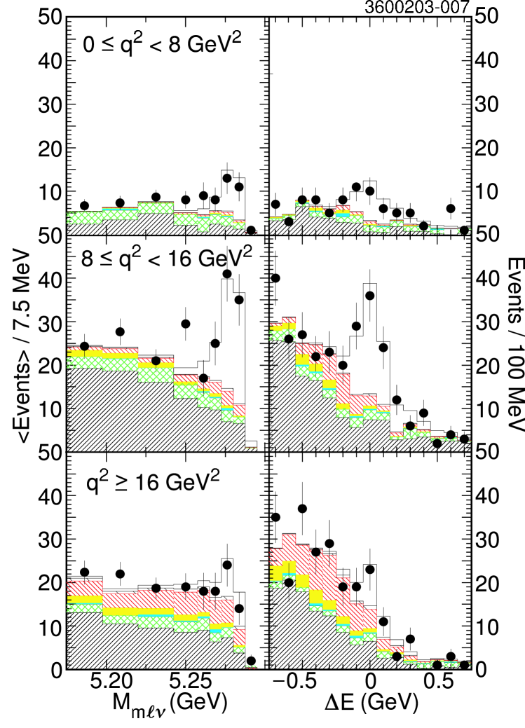
Figure 3: $M_{m\ell\nu}$ (left) and $\Delta E$ (right) in the $\Delta E$ and $M_{m\ell\nu}$ “signal” band requiring $\Delta Q=0$ for the combined $\pi^{\pm},\pi^{0}$ modes. The points are the on-resonance data. The histogram components, from bottom to top, are $b\to c$ (fine $45^{\circ}$ hatch), continuum (grey or green cross hatch), fake leptons (cyan or dark grey), feed down from other $B\to X_{u}\ell\nu$ modes (yellow or light grey), cross feed from the vector and $\eta$ modes into the reconstructed modes (red or black fine $135^{\circ}$ hatch), cross feed among the $\pi$ modes (coarse $135^{\circ}$ hatch), and signal (open). The normalizations are from the nominal fit.

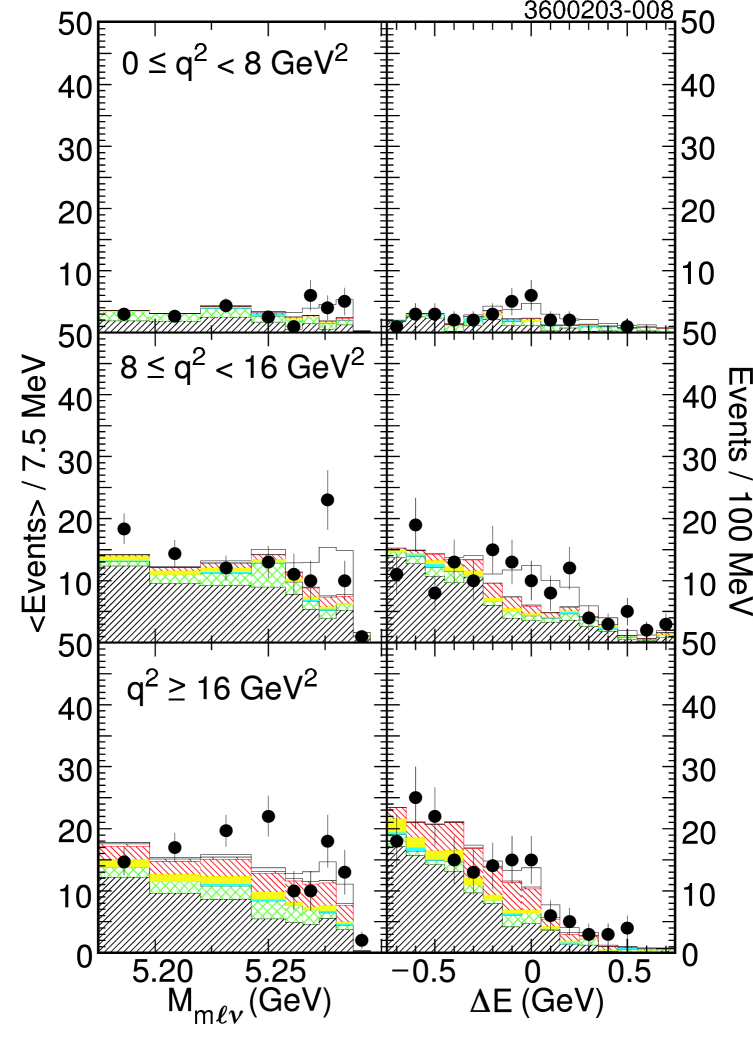
Figure 4: $M_{m\ell\nu}$ (left) and $\Delta E$ (right) in the $\Delta E$ and $M_{m\ell\nu}$ “signal” band requiring $|\Delta Q|=1$ for the combined $\pi^{\pm},\pi^{0}$ modes. The points are the on-resonance data. See Fig. 3 for component and normalization descriptions.

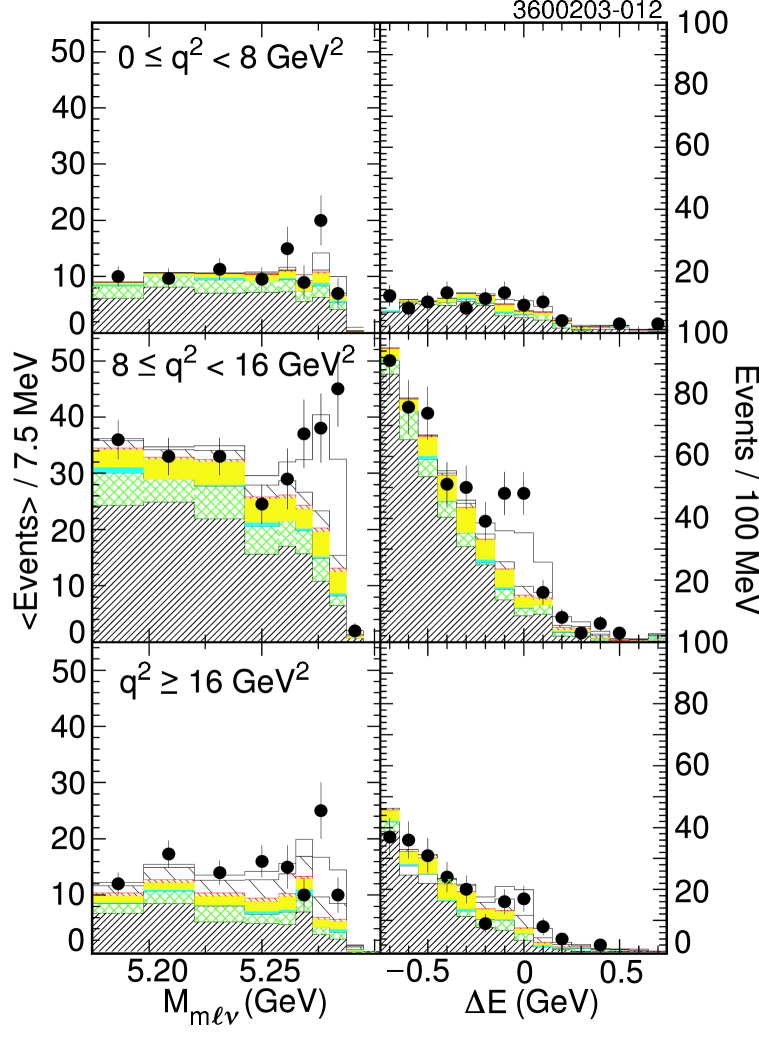
Figure 5: $M_{m\ell\nu}$ (left) and $\Delta E$ (right) in the $\Delta E$ and $M_{m\ell\nu}$ “signal” band requiring $\Delta Q=0$ for the combined $\rho^{\pm},\rho^{0}$ modes with the requirement $p_{\ell}>1.5\ \mathrm{GeV}/c$ in the vector modes. The points are the on-resonance data. The hatching and normalization are as in Fig. 3 except that the red or black fine $135^{\circ}$ hatch cross feed component is from $\pi$ and $\eta$ modes into the $\rho$ modes, and the coarse hatch cross feed component is from among the vector modes.

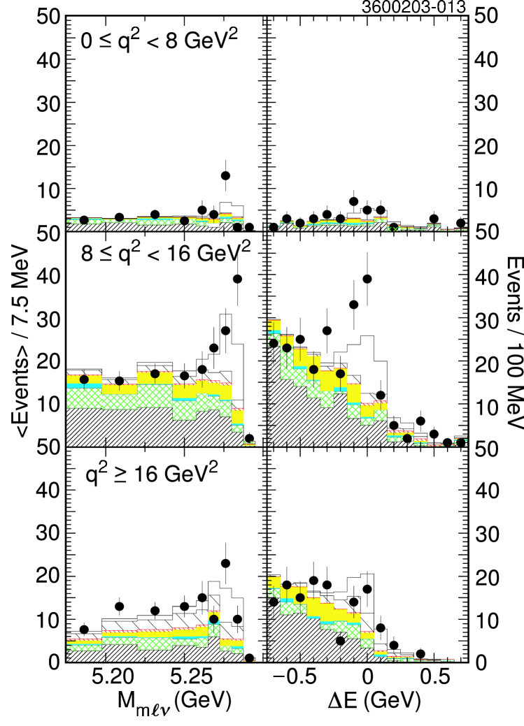
Figure 6: $M_{m\ell\nu}$ (left) and $\Delta E$ (right) in the $\Delta E$ and $M_{m\ell\nu}$ “signal” band requiring $\Delta Q=0$ for the combined $\rho^{\pm},\rho^{0}$ modes with the requirement $p_{\ell}>2.0\ \mathrm{GeV}/c$ in the vector modes. The points are the on-resonance data. The hatching is as in Fig. 5. The normalizations come from the fit with the corresponding lepton momentum requirement.

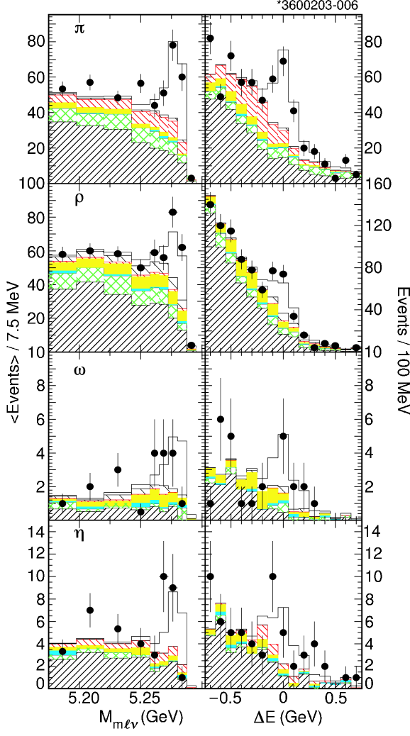
Figure 7: $M_{m\ell\nu}$ (left), $\Delta E$ (right) in the $\Delta E$ and $M_{m\ell\nu}$ signal bands for $\Delta Q=0$ and summed over the entire $q^{2}$ range for the combined $\pi$ modes (top), $\rho$ modes (row 2), $\omega$ (row 3), and $\eta$ (bottom) modes. See Figs. 3 and 5 for component and normalization descriptions. For $\eta$ there is only a single cross–feed component from the non–$\eta$ modes (red or black fine $135^{\circ}$ hatch.

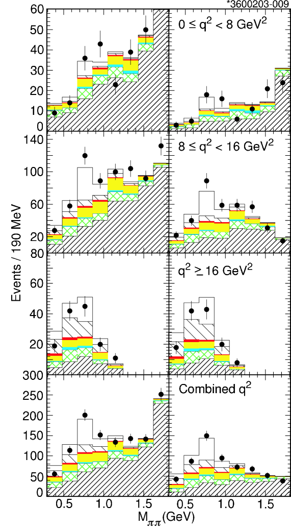
Figure 8: Reconstructed mass distributions for $\rho\to\pi\pi$ in the $(M_{m\ell\nu},\Delta E)$ signal bin for the two analyses with $p_{\ell}>1.5\ \mathrm{GeV}/c$ in the vector modes (left) and with $p_{\ell}>2.0\ \mathrm{GeV}/c$ (right). See Fig. 5 for component and normalization descriptions.

The lepton momentum spectra and $\cos\theta_{W\ell}$ distributions in the $(M_{m\ell\nu},\Delta E)$ signal bin are shown in Figures 9 and 10. This information is not used in the fit, but shows good agreement with the signals preferred in the fit. The $\pi\pi$ mass distribution for the combined $\rho\ell\nu$ modes is shown in Fig. 8.

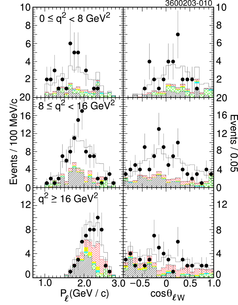
Figure 9: Charged lepton momentum spectrum (left) and $\cos\theta_{W\ell}$ (right) for the combined $\pi\ell\nu$ modes in the three $q^{2}$ intervals. See Fig. 3 for component and normalization descriptions.

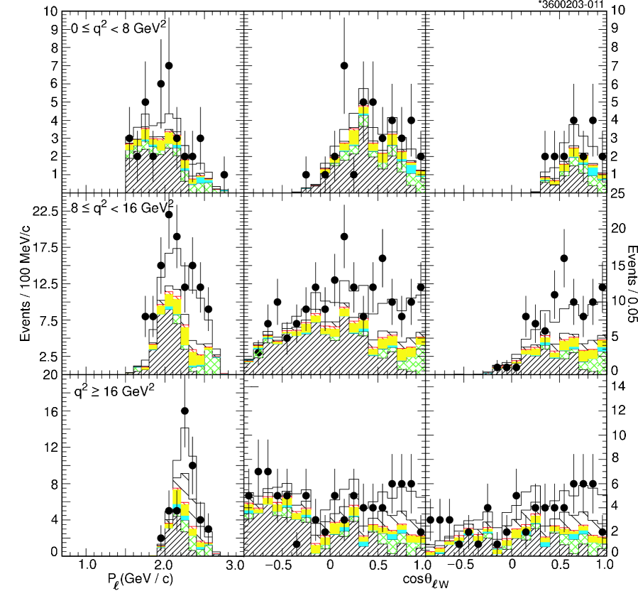
Figure 10: Charged lepton momentum spectrum (left) and $\cos\theta_{W\ell}$ distributions for the combined $\rho\ell\nu$ modes in the three $q^{2}$ intervals. The $\cos\theta_{W\ell}$ distribution is shown for both the analysis with $p_{\ell}>1.5\ \mathrm{GeV}/c$ in the vector modes (center) and for $p_{\ell}>2.0\ \mathrm{GeV}/c$ (right). See Fig. 5 for component and normalization descriptions.

The branching fractions from the nominal fit are summarized in Table 3. The results are remarkably stable as the lepton momentum requirement in the vector modes is varied. The greatest variation is observed in the lowest $q^{2}$ interval in the $\rho\ell\nu$ modes, which we expected because of the larger role that interference between the form factors plays in that region.

Use of a $\chi^{2}$–based fitting procedure produced similar results, though we saw clearly that low statistics bins had an undue influence on the results of that fitter. Such sensitivity was eliminated with the log likelihood minimization.

Table 3: Summary of branching fractions from the nominal fit using the Ball’01 and Ball’98 form factors for the $\pi$ and $\rho$ modes, respectively. The first uncertainties are statistical and the second systematic (see Section V). The results for the fits with more restrictive lepton momentum requirements in the vector modes are also shown. The $q^{2}$ intervals are specified in GeV².

Mode	${\cal B}_{q^{2}\,\mathrm{interval}}$	analysis requirement (vector modes)
	$\times 10^{4}$	$p_{\ell}>1.5\ \mathrm{GeV}/c$	$p_{\ell}>1.75\ \mathrm{GeV}/c$	$p_{\ell}>2.0\ \mathrm{GeV}/c$
$B^{0}\to\pi^{-}\ell^{+}\nu$	${\cal B}_{\text{total}}$	$1.33\pm 0.18\pm 0.11$	$1.31\pm 0.18\pm 0.11$	$1.32\pm 0.18\pm 0.12$
	${\cal B}_{<8}$	$0.43\pm 0.11\pm 0.05$	$0.43\pm 0.11\pm 0.05$	$0.42\pm 0.11\pm 0.05$
	${\cal B}_{8-16}$	$0.65\pm 0.11\pm 0.07$	$0.65\pm 0.11\pm 0.07$	$0.66\pm 0.11\pm 0.07$
	${\cal B}_{\geq 16}$	$0.25\pm 0.09\pm 0.04$	$0.24\pm 0.09\pm 0.04$	$0.24\pm 0.09\pm 0.05$
$B^{0}\to\rho^{-}\ell^{+}\nu$	${\cal B}_{\text{total}}$	$2.17\pm 0.34\;^{+0.47}_{-0.54}$	$2.34\pm 0.34\;^{+0.43}_{-0.51}$	$2.29\pm 0.35\;^{+0.40}_{-0.49}$
	${\cal B}_{<8}$	$0.43\pm 0.20\;^{+0.23}_{-0.23}$	$0.50\pm 0.20\;^{+0.21}_{-0.22}$	$0.62\pm 0.22\;^{+0.22}_{-0.23}$
	${\cal B}_{8-16}$	$1.24\pm 0.26\;^{+0.27}_{-0.33}$	$1.32\pm 0.26\;^{+0.26}_{-0.29}$	$1.11\pm 0.25\;^{+0.23}_{-0.25}$
	${\cal B}_{\geq 16}$	$0.50\pm 0.10\;^{+0.08}_{-0.11}$	$0.52\pm 0.10\;^{+0.08}_{-0.10}$	$0.56\pm 0.10\;^{+0.07}_{-0.09}$
$B^{+}\to\eta\ell^{+}\nu$	${\cal B}_{\text{total}}$	$0.84\pm 0.31\pm 0.16$	$0.84\pm 0.31\pm 0.16$	$0.83\pm 0.31\pm 0.15$

The increase in $-2\ln{\cal L}$ from best fit to ${\cal B}(B^{+}\rightarrow\eta\ell^{+}\nu)=0$ is 10.4, corresponding roughly to a 3.2$\sigma$ statistical significance.

V Experimental systematics

Table 4: Contributions to the systematic error (%) in each total and partial branching fraction (${\cal B}$). Simulation of the detector and the second $B$ contribute to $\nu$ simulation.

	$\pi\ell\nu$				$\rho(\omega)\ell\nu$
		$q^{2}$ interval (GeV2)				$q^{2}$ interval (GeV2)
Systematic	${\cal B}_{\text{total}}$	$<8$	$8-16$	$\geq 16$	${\cal B}_{\text{total}}$	$<8$	$8-16$	$\geq 16$	$\eta$
$\nu$ simulation	6.8	10.5	9.2	17.2	18.7	41.7	19.4	13.5	17.3
$B\to D/D^{*}/D^{**}/D^{\rm NR}X\ell\nu$	1.7	2.5	1.9	3.2	2.0	21.4	4.7	4.2	5.5
$B\to X_{u}\ell\nu$ feed down	0.5	3.0	1.8	1.9	8.3	23.8	6.1	5.6	1.6
Continuum smoothing	1.0	2.0	0.2	2.0	3.0	10.0	1.0	2.0	2.0
Fakes	3.0	3.0	3.0	3.0	3.0	3.0	3.0	3.0	3.0
Lepton ID	2.0	2.0	2.0	2.0	2.0	2.0	2.0	2.0	2.0
$f_{+-}/f_{00}$	2.4	2.6	2.3	2.2	0.0	2.5	1.0	0.1	4.1
$\tau_{B^{+}}/\tau_{B^{0}}$	0.2	0.1	0.3	0.5	2.1	4.2	1.4	2.1	1.4
Isospin	0.0	0.0	0.0	0.2	2.4	1.9	2.7	2.3	0.1
Luminosity	2.0	2.0	2.0	2.0	2.0	2.0	2.0	2.0	2.0
Upper	8.6	12.4	10.7	18.3	21.4	53.9	21.5	16.2	19.3
Non Resonant	–	–	–	–	-13	-9	-15	-14
Lower	8.6	12.4	10.7	18.3	25.1	54.7	26.2	21.4	19.3

Table 4 summarizes the contributions to the systematic errors for the nominal analysis. The dominant contribution is from uncertainties in “$\nu$ simulation,” which includes inaccuracies in detector simulation and uncertainty in the decay model of the nonsignal $B$. The breakdown of “$\nu$ simulation” into its component parts is given in Table 5 (and with lepton momentum cuts for vector modes of 1.75 GeV/$c$ and 2.0 GeV/$c$, in Tables 6 and 7, respectively).

We investigated the systematic uncertainties in “$\nu$ simulation” by modifying, for each systematic contribution under consideration, the reconstruction output of all of the Monte Carlo samples used in the fit. Using independent studies by CLEO for this and other analyses, our modifications reflected the uncertainties in charged-particle-finding and photon-finding efficiencies, simulation of false charged particles and photons, charged particle momentum resolution, photon energy resolution, hadronic shower simulation, and charged particle identification. In addition, we reweighted the Monte Carlo samples to account for the uncertainties in the rate and spectrum for $K^{0}_{L}$ production in $B$ decay and in the process $b\to c\to s\ell\nu$, both of which affect the background rate into the signal region. The full MC samples were re-analyzed for each variation to allow for leakage of events across the selection boundaries. The variations are described in more detail in Appendix A.

For many of the variations in the simulation, we expect a cancellation between the change in the signal yield and the change in the efficiency. (Note that we are not changing the analysis – the data yields remain unchanged.) The cancellation arises as follows. If we degrade the reconstructed neutrino, the efficiency for signal is reduced, but background tends to smear more readily into the signal region. Hence the signal yield also tends to be reduced, offsetting the change in efficiency. Because of the expected imperfections in our simulation, we do not expect the observed cancellation to be perfectly reliable. For each variation, we therefore assign an additional uncertainty in the branching fraction so that the total fractional uncertainty estimate is

$$\sigma=\sigma_{\mathrm{BR}}\oplus\frac{\sqrt{2}}{3}\min(\sigma_{\mathrm{yield}},\sigma_{\mathrm{eff}}).$$ (7)

In this expression, $\sigma_{\mathrm{BR}}$ is the percentage change in the branching fraction from the fit, $\sigma_{\mathrm{yield}}$ is the percentage change in the “signal bin” yield, and $\sigma_{\mathrm{eff}}$ is the percentage change in the “signal bin” efficiency. For complete cancellation ($\sigma_{\mathrm{yield}}=\sigma_{\mathrm{eff}}$; $\sigma_{\mathrm{BR}}=0$), the additional term amounts to the addition in quadrature of one third of the change observed in the yield and in the efficiency. When no cancellation is expected, the additional term is zero. The values for $\sigma_{\mathrm{yield}}$ and $\sigma_{\mathrm{eff}}$ are estimated by examining the changes in the “signal bin.”

Note that because of correlations between the three $q^{2}$ intervals in a given mode, the sum of the modes tends to be less sensitive to the systematic variations than the individual intervals themselves.

Consider now the items in Table 4 other than “$\nu$ simulation.” We reweight the Monte Carlo to allow variation in the relative rates for $D\ell\nu$, $D^{*}\ell\nu$, and $(Dn\pi)\ell\nu$, both for resonant $Dn\pi$ and nonresonant $Dn\pi$. We vary the rates by $\pm 8\%$, $\pm 6\%$, $\pm 30\%$, and $\pm 30\%$, respectively. Note that if we completely eliminate any one of these charmed modes except $D^{*}\ell\nu$, the total branching fractions for $\pi$ and $\rho$ remain stable within 4% of themselves, which demonstrates that we are quite insensitive to the details of the poorly measured nonresonant and resonant $(Dn\pi$) modes. Zeroing $D^{*}\ell\nu$ completely causes changes of only 15%, further demonstrating our insensitivity to the detailed modeling of the $b\to c\ell\nu$ process.

For the $B\to X_{u}\ell\nu$ background, we evaluate two contributions to the systematic uncertainty. First, we vary the nonperturbative parameters of the inclusive spectrum used to drive the $X_{u}\ell\nu$ simulation within the uncertainties obtained from the $B\to X_{s}\gamma$ analysis that were used in the recent end-point measurement bb:bsgamm_exp ; bb:new_endpoint . That analysis provides an error ellipse for the HQET parameters $\lambda_{1}$ versus $\overline{\Lambda}$, and we choose the points on that ellipse that make the maximal change. The second contribution regards uncertainty in the hadronization of the final state light quarks. We change from our model that marries the ISGW II exclusive and OPE inclusive calculations (see previous section) to a purely “nonresonant” hadronization procedure (similar to that of JETSET bb:jetset ). The hadronization is nonresonant in the sense that single hadron final states (e.g., $a_{1}\ell\nu$) are not produced. Resonances can appear in the multihadron final state (e.g., $\rho\pi\ell\nu$). To avoid overlap of the nonresonant sample with the signal modes, we eliminate $B\to X_{u}\ell\nu$ events with a low mass $\pi\pi$ final state. The uncertainties presented correspond to a minimum $M_{\pi\pi}$ of 1 GeV. Variation of that threshold over the 0.9 – 1.1 GeV range results in similar systematic estimates. As a crosscheck, we have also used the strictly resonant description of ISGW II, which yields results consistent with our uncertainty estimates.

We have used different normalization schemes for the $B\to X_{u}\ell\nu$ background to check the sensitivity of the results under the normalization procedure. If we drop the end-point branching fraction constraint but still allow the normalization to float, we see only minor shifts in the results and the end-point branching fraction predicted by the fit is within one standard deviation of the measured value. We have also used an iterative procedure, where we fix the $B\to X_{u}\ell\nu$ normalization in the fit, but update that normalization until the fit’s predicted end-point branching fraction converges to the central value (and then to $\pm 1$ standard deviation) of the CLEO measurement. This procedure also gave consistent results.

As Table 4 shows, uncertainty in the $B\to X_{u}\ell\nu$ feed down contributes little to the systematic error on $\pi\ell\nu$ and $\eta\ell\nu$. For the $\rho\ell\nu$ rate, however, the contribution is substantial.

Our nominal fit assumed equal production of charged and neutral $B$ mesons: $f_{+-}/f_{00}=1$. We varied this fraction over the one standard deviation range indicated by the recent CLEO result $f_{+-}/f_{00}=1.04\pm 0.08$ silvia . The relationship enters both in the fit to implement the isospin constraint and in the branching fraction calculation to calculate the number of $B^{0}$ mesons. We used the measured ratio of $B$ meson lifetimes, $\tau_{B^{+}}/\tau_{B^{0}}=1.083\pm 0.017$, which we varied by one standard deviation to assess the associated uncertainty. The ratio comes into the normalization of the neutral modes versus the charged modes. We have also varied the isospin assumption. In the nominal fit we used a ratio of 2. For the systematic estimate we lowered the $\rho^{+}:\rho^{0}$ ratio down to 1.43, as suggested by Diaz-Cruz bb:DiazCruz . The deviation arises from $\rho^{0}--\omega$ mixing coupled with the large $\rho^{0}$ width. Because of the small $\eta$ and $\omega$ widths, we expect negligible deviation from the the ideal factor of two for the other two ratios used.

The uncertainties related to lepton identification are estimated by varying the measured hadronic fake rates within their uncertainties and by applying the uncertainty in the measurement of the average lepton identification efficiency. Lepton–fake uncertainties are measured in the data as a function of momentum using cleanly tagged hadronic samples, including $K_{S}\to\pi^{+}\pi^{-}$ and $D^{*\pm}\to\pi^{\pm}D^{0}$, $D^{0}\to K^{\pm}\pi^{\mp}$.

Finally, we assessed our smoothing technique for the continuum data sample. Recall that we use the off–resonance data distrubution with relaxed continuum–suppression combined with the expected shape change over the fitted $\Delta E$ and $M_{m\ell\nu}$ region that is induced by the relaxation. We biased the Monte Carlo prediction for the shape change by the statistical uncertainty in the parameterization for each of the fitted ($\Delta E$, $M_{m\ell\nu}$) distributions. The uncertainties come from fluctuating all distributions coherently to induce the maximum change.

Table 5: Percentage change in results for a fit with a modified simulation relative to a fit to the nominal MC simulation for each of the variations contributing to the simulation systematic uncertainty. The vector modes were analyzed with the requirement $p_{\ell}>1.5\ \mathrm{GeV}/c$. The last row shows the quadrature sum of the changes.

variation	$\pi^{-}\ell^{+}\nu$				$\rho^{-}\ell^{+}\nu$				$\eta\ell\nu$
	total	$q^{2}<8$	$8\leq q^{2}<16$	$q^{2}\geq 16$	total	$q^{2}<8$	$8\leq q^{2}<16$	$q^{2}\geq 16$	total
$\gamma$ eff.	2.6	7.0	2.7	9.1	11.1	11.9	11.1	10.6	5.7
$\gamma$ resol.	4.1	2.9	5.4	2.3	2.9	3.7	2.3	4.2	9.6
$K_{L}$ shower	1.3	1.0	1.4	1.4	6.0	8.4	7.2	1.6	2.7
particle ID	1.9	2.5	3.0	6.3	8.2	27.5	6.9	1.1	0.2
split-off rejection	1.5	2.9	3.0	5.0	1.2	9.4	1.8	2.5	5.5
track eff.	3.7	4.5	4.2	2.6	8.6	13.3	9.5	3.4	9.5
track resol.	1.0	1.8	2.4	11.2	6.2	12.7	6.0	2.7	0.9
split-off sim.	0.4	1.4	0.5	2.3	1.0	10.4	1.0	4.7	6.0
$K_{L}$ production	0.2	0.1	0.2	0.4	0.1	0.8	0.1	0.3	0.1
$\nu$ production	0.5	3.5	2.2	2.0	0.6	15.1	4.1	0.9	2.9
Total	6.8	10.4	9.2	17.2	18.7	41.7	19.4	13.5	17.3

Table 6: Percentage change in results for a fit with a modified simulation relative to a fit to the nominal MC simulation for each of the variations contributing to the simulation systematic uncertainty. The vector modes were analyzed with the requirement $p_{\ell}>1.75\ \mathrm{GeV}/c$. The last row shows the quadrature sum of the changes.

variation	$\pi^{-}\ell^{+}\nu$				$\rho^{-}\ell^{+}\nu$				$\eta\ell\nu$
	total	$q^{2}<8$	$8\leq q^{2}<16$	$q^{2}\geq 16$	total	$q^{2}<8$	$8\leq q^{2}<16$	$q^{2}\geq 16$	total
$\gamma$ eff.	2.6	6.8	2.8	9.3	9.7	8.9	10.3	9.0	5.9
$\gamma$ resol.	4.0	2.7	5.4	2.4	3.2	4.6	2.7	4.1	9.7
$K_{L}$ shower	1.4	1.0	1.3	1.7	4.6	4.8	6.1	0.5	2.6
particle ID	1.8	2.7	3.0	6.4	7.8	24.2	6.9	1.0	0.0
split-off rejection	1.5	2.5	3.1	4.7	0.5	1.7	0.9	2.4	5.0
track eff.	3.7	4.3	4.2	2.6	8.4	11.9	9.7	3.4	9.7
track resol.	1.0	1.8	2.6	11.4	4.6	8.1	4.9	1.8	0.8
split-off sim.	0.4	1.5	0.5	2.4	1.1	1.5	0.3	5.3	5.3
$K_{L}$ production	0.2	0.1	0.1	0.4	0.1	0.7	0.1	0.3	0.0
$\nu$ production	0.5	3.5	2.3	2.2	0.8	13.3	3.1	0.6	2.7
Total	6.7	10.2	9.3	17.4	16.7	33.1	18.0	12.2	17.0

Table 7: Percentage change in results for a fit with a modified simulation relative to a fit to the nominal MC simulation for each of the variations contributing to the simulation systematic uncertainty. The vector modes were analyzed with the requirement $p_{\ell}>2.0\ \mathrm{GeV}/c$. The last row shows the quadrature sum of the changes.

variation	$\pi^{-}\ell^{+}\nu$				$\rho^{-}\ell^{+}\nu$				$\eta\ell\nu$
	total	$q^{2}<8$	$8\leq q^{2}<16$	$q^{2}\geq 16$	total	$q^{2}<8$	$8\leq q^{2}<16$	$q^{2}\geq 16$	total
$\gamma$ eff.	2.6	6.8	2.7	8.8	12.3	12.3	14.6	8.3	5.9
$\gamma$ resol.	4.2	2.7	5.4	3.9	1.3	1.1	2.3	1.0	9.3
$K_{L}$ shower	1.3	0.9	1.7	1.7	2.4	1.8	3.2	1.2	2.6
particle ID	1.9	2.7	3.1	6.4	7.0	15.6	8.1	1.1	0.4
split-off rejection	1.7	2.7	3.0	5.9	1.8	1.5	2.9	0.7	5.7
track eff.	3.9	4.3	4.5	2.4	4.1	4.7	6.5	1.8	9.2
track resol.	1.0	1.5	3.0	11.8	3.6	8.2	2.4	2.7	1.0
split-off sim.	0.4	1.6	0.5	3.1	1.9	6.6	2.8	3.0	5.2
$K_{L}$ production	0.2	0.2	0.1	0.4	0.2	0.5	0.2	0.4	0.1
$\nu$ production	0.6	3.5	2.4	2.6	0.7	6.3	1.5	0.6	2.1
Total	7.0	10.2	9.7	18.2	15.7	23.9	18.9	9.7	16.7

In the $\rho$ modes, there is an additional uncertainty from the unknown contribution of nonresonant $\pi\pi\ell\nu$ decays. While little is known about these decays, we can provide a framework for limiting those contributions through the study of reconstructed $\pi^{0}\pi^{0}\ell^{\pm}\nu$ decays and the consideration of Bose symmetry, isospin, and angular momentum. The $B\to X_{u}\ell\nu$ decay results, before hadronization, in two final-state light quarks. These can have either isospin $I=0$ or $I=1$. Because final-state interactions preserve isospin, a final $\pi\pi$ state is also restricted to $I=0$ or $I=1$. From Bose symmetry considerations, the $\pi\pi$ state must have angular momentum $L$ even for $I=0$ and $L$ odd for $I=1$. Isospin considerations then imply

$$\begin{array}[]{rr}I=1,L\ \textrm{odd}&\pi^{\pm}\pi^{0}:\pi^{+}\pi^{-}:\pi^{0}\pi^{0}=2:1:0\\ I=0,L\ \textrm{even}&\pi^{\pm}\pi^{0}:\pi^{+}\pi^{-}:\pi^{0}\pi^{0}=0:2:1.\end{array}$$

Assuming that the $L=3,5,...$ configurations are suppressed relative to the $L=1$ configuration, we can use $e^{+}e^{-}$ scattering data and $\tau$ decay data to conclude that the $I=1,L\ \textrm{odd}$ component is completely dominated by the $\rho$. A significant nonresonant contribution would therefore come via the $I=0,L\ \textrm{even}$ channel. With the $I=0$ rate parameterized by $\alpha$, we expect partial widths in the ratios

$$\pi^{\pm}\pi^{0}:\pi^{+}\pi^{-}:\pi^{0}\pi^{0}=2:1+2\alpha:\alpha.$$

To estimate the systematic due to an unknown nonresonant $\pi\pi\ell\nu$ contribution, we look for a component, after event selection, that could mimic a $\rho\ell\nu$. To constrain such a contribution, we add the mode $\pi^{0}\pi^{0}\ell\nu$ to the fit. Procedurally, we generate $\pi^{0}\pi^{0}\ell\nu$ using the $\rho$ lineshape and the $\rho\ell\nu$ form factors. We then perform fits with the usual isospin constraint on the partial widths ($\rho^{\pm}:\rho^{0}=2:1$) replaced with the $\pi\pi$ ratios given above. While the most relevant fit for the extraction of a systematic uncertainty number has the parameter $\alpha$ floating, we also fix $\alpha=0$ to test the fit quality under the assumption that observed $\pi^{0}\pi^{0}\ell\nu$ yields are consistent with cross feed from other modes and the other standard backgrounds.

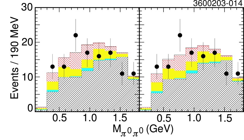
Figure 11: The $\pi^{0}\pi^{0}$ mass distribution from the reconstructed $\pi^{0}\pi^{0}\ell^{\pm}\nu$ “signal bin” from the nominal fit (left) and from the fit including a $\pi^{0}\pi^{0}\ell^{\pm}\nu$ signal component (right) as described in the text. The points are the on-resonance data. The histogram components, from bottom to top, are $b\to c$ (fine $45^{\circ}$ hatch), continuum (grey or green cross hatch), fake leptons (cyan or dark grey), feed down from other $B\to X_{u}\ell\nu$ modes (yellow or light grey), cross feed from the signal modes into the reconstructed modes (red or black fine $135^{\circ}$ hatch), and signal (open). The normalizations are from the corresponding fits.

In the fits, the $\pi^{0}\pi^{0}\ell\nu$ mode is treated like the $\omega$ mode. Only the sum of the three $q^{2}$ intervals contributes to the likelihood, but the signal Monte Carlo is scaled in each $q^{2}$ interval separately to maintain the above $\pi\pi$ ratios from one interval to the next. Figure 11 shows the projection onto the $m_{\pi^{0}\pi^{0}}$ distribution for fits with and without a $\pi^{0}\pi^{0}\ell\nu$ signal component. Note that the fit included data only from the three bins in the range $0.485\leq m_{\pi^{0}\pi^{0}}<1.055$ GeV. The fit quality is excellent when the reconstructed $\pi^{0}\pi^{0}\ell\nu$ mode is included but the $\pi^{0}\pi^{0}\ell\nu$ signal is forced to zero. Table 8 summarizes the observed changes in the $\rho^{-}\ell^{+}\nu$ branching fraction when we float the $\pi^{0}\pi^{0}\ell\nu$ signal component. The resulting $\pi^{0}\pi^{0}\ell\nu$ yield is consistent with zero. The shifts in the various $\rho\ell\nu$ branching fractions are larger effects than the increase in their errors due to correlations with the $\pi^{0}\pi^{0}\ell\nu$. We thus take the shifts as the estimate of the uncertainty. The pseudoscalar modes shift negligibly.

Table 8: Comparisons of the $\rho^{-}\ell^{+}\nu$ branching fractions when the $\pi^{0}\pi^{0}\ell\nu$ mode and component are added. The parameter $\alpha$ that normalizes the $\pi^{0}\pi^{0}\ell\nu$ component is described in the text. The percentage change relative to the standard fits in Table 3 are indicated in parentheses below the branching fractions.

analysis	$\alpha$	${\cal B}(B\to\rho\ell\nu)$	${\cal B}_{q^{2}<8\ \mathrm{GeV}^{2}}$	${\cal B}_{8\leq q^{2}<16\ \mathrm{GeV}^{2}}$	${\cal B}_{q^{2}\geq 16\ \mathrm{GeV}^{2}}$	$\chi^{2}$/dof
		($10^{-4}$)	($10^{-4}$)	($10^{-4}$)
$p_{\ell}>1.5\ \mathrm{GeV}/c$	$0.25\pm 0.21$	$1.88\pm 0.35$	$0.393\pm 0.209$	$1.055\pm 0.261$	$0.428\pm 0.099$	273.7 / (280-21)
		(-13%)	(-9%)	(-15%)	(-14%)
$p_{\ell}>1.75\ \mathrm{GeV}/c$	$0.22\pm 0.18$	$2.06\pm 0.35$	$0.455\pm 0.216$	$1.153\pm 0.259$	$0.455\pm 0.099$	271.6 / (280-21)
		(-12%)	(-8%)	(-9%)	(-11%)
$p_{\ell}>2.0\ \mathrm{GeV}/c$	$0.18\pm 0.13$	$2.17\pm 0.36$	$0.669\pm 0.249$	$1.009\pm 0.241$	$0.496\pm 0.097$	281.1 / (280-21)
		(-5%)	(8%)	(-9%)	(-11%)

In addition to the variations above, we have performed numerous systematic checks, including variation of the selection criteria and investigation of electron and muon samples separately. We have also investigated tighter momentum requirements in the pseudoscalar modes. The observed variations were in general consistent within the uncertainties resulting from the statistical changes.

VI Dependence of branching fractions on form factors

Table 9: Branching fractions ${\cal B}(B^{0}\to\pi^{-}\ell^{+}\nu)$ obtained under variation of the $\pi$ and $\rho/\omega\ell\nu$ form-factor models. Shown are the results for the total branching fraction, the partial branching fraction in each $q^{2}$ bin, and the $-2\ln L$ for the fit. Branching fraction uncertainties are statistical only. The estimated model dependence is indicated after each set of variations. All branching fractions are in units of $10^{-4}$. The $\pi$ model variations are all presented for the analysis with the $p_{\ell}>1.5\ \mathrm{GeV}/c$ requirement on the vector modes.

			$q^{2}$ interval (GeV2)
$\pi$ Model	$\rho$ Model	${\cal B}_{\text{total}}$	${\cal B}_{<8}$	${\cal B}_{8-16}$	${\cal B}_{\geq 16}$	$-2\ln L$
Ball’01	Ball’98	$1.327\pm 0.177$	$0.431\pm 0.106$	$0.651\pm 0.105$	$0.245\pm 0.094$	240.3
ISGW2	Ball’98	$1.327\pm 0.176$	$0.431\pm 0.107$	$0.660\pm 0.106$	$0.236\pm 0.09$	240.7
SPD	Ball’98	$1.315\pm 0.173$	$0.436\pm 0.106$	$0.650\pm 0.105$	$0.229\pm 0.088$	239.8
$1.7\times\mathrm{RMS}_{\pi\,\mathrm{FF}}$		0.01	0.004	0.01	0.01
Ball’01	Ball’98	$1.33\pm 0.18$	$0.43\pm 0.11$	$0.65\pm 0.11$	$0.25\pm 0.09$	240.3
Ball’01	ISGW2	$1.41\pm 0.18$	$0.45\pm 0.11$	$0.69\pm 0.10$	$0.27\pm 0.09$	239.4
Ball’01	Melikhov’00	$1.30\pm 0.18$	$0.43\pm 0.11$	$0.65\pm 0.11$	$0.22\pm 0.09$	240.2
Ball’01	UKQCD’98	$1.36\pm 0.18$	$0.44\pm 0.11$	$0.66\pm 0.11$	$0.26\pm 0.09$	239.3
$1.7\times\mathrm{RMS}_{\rho\,\mathrm{FF}}$		0.07	0.01	0.03	0.03

Table 10: Branching fractions ${\cal B}(B^{0}\to\rho^{-}\ell^{+}\nu)$ obtained under variation of the $\pi\ell\nu$ and $\rho/\omega\ell\nu$ form-factor models. Shown are the results for the total branching fraction, the partial branching fraction in each $q^{2}$ bin, and the $-2\ln L$ for the fit. Branching fraction uncertainties are statistical only. The estimated model dependence is indicated after each set of variations. All branching fractions are in units of $10^{-4}$. The $\pi$ model variations are all presented for the analysis with the $p_{\ell}>1.5\ \mathrm{GeV}/c$ requirement on the vector modes. For the vector mode form-factor variation, we present the results for all three momentum requirements.

			$q^{2}$ interval (GeV2)
$\pi$ Model	$\rho$ Model	${\cal B}_{\text{total}}$	${\cal B}_{<8}$	${\cal B}_{8-16}$	${\cal B}_{\geq 16}$	$-2\ln L$
Ball’01	Ball’98	$2.172\pm 0.338$	$0.429\pm 0.198$	$1.244\pm 0.256$	$0.499\pm 0.097$	240.3
ISGW2	Ball’98	$2.176\pm 0.338$	$0.430\pm 0.198$	$1.248\pm 0.256$	$0.499\pm 0.098$	240.7
SPD	Ball’98	$2.169\pm 0.338$	$0.420\pm 0.198$	$1.250\pm 0.256$	$0.499\pm 0.098$	239.8
$1.7\times\mathrm{RMS}_{\pi\,\mathrm{FF}}$		0.01	0.01	0.004	0.004
$p_{\ell}>1.5\ \mathrm{GeV}/c$
Ball’01	Ball’98	$2.17\pm 0.34$	$0.43\pm 0.20$	$1.24\pm 0.26$	$0.50\pm 0.10$	240.3
Ball’01	ISGW2	$1.91\pm 0.28$	$0.30\pm 0.13$	$1.14\pm 0.23$	$0.47\pm 0.10$	239.4
Ball’01	Melikhov’00	$2.56\pm 0.37$	$0.33\pm 0.15$	$1.49\pm 0.31$	$0.75\pm 0.14$	240.2
Ball’01	UKQCD’98	$2.08\pm 0.32$	$0.39\pm 0.17$	$1.21\pm 0.25$	$0.49\pm 0.10$	239.3
$1.7\times\mathrm{RMS}_{\rho\,\mathrm{FF}}$		0.41	0.09	0.22	0.19
$p_{\ell}>1.75\ \mathrm{GeV}/c$
Ball’01	Ball’98	$2.34\pm 0.34$	$0.50\pm 0.20$	$1.32\pm 0.26$	$0.52\pm 0.10$	241.6
Ball’01	ISGW2	$2.03\pm 0.28$	$0.34\pm 0.13$	$1.20\pm 0.23$	$0.49\pm 0.10$	240.3
Ball’01	Melikhov’00	$2.74\pm 0.37$	$0.38\pm 0.16$	$1.58\pm 0.31$	$0.78\pm 0.14$	241.4
Ball’01	UKQCD’98	$2.23\pm 0.32$	$0.45\pm 0.18$	$1.28\pm 0.25$	$0.51\pm 0.10$	240.4
$1.7\times\mathrm{RMS}_{\rho\,\mathrm{FF}}$		0.44	0.11	0.24	0.20
$p_{\ell}>2.0\ \mathrm{GeV}/c$
Ball’01	Ball’98	$2.29\pm 0.35$	$0.62\pm 0.22$	$1.11\pm 0.25$	$0.56\pm 0.10$	244.2
Ball’01	ISGW2	$1.89\pm 0.27$	$0.38\pm 0.13$	$0.98\pm 0.22$	$0.54\pm 0.09$	243.4
Ball’01	Melikhov’00	$2.66\pm 0.38$	$0.48\pm 0.17$	$1.36\pm 0.31$	$0.83\pm 0.14$	244.6
Ball’01	UKQCD’98	$2.15\pm 0.32$	$0.54\pm 0.19$	$1.07\pm 0.24$	$0.55\pm 0.09$	243.3
$1.7\times\mathrm{RMS}_{\rho\,\mathrm{FF}}$		0.47	0.15	0.24	0.21

In the original measurement of the exclusive charmless branching fractions bb:lkg_cleo_exclusive , there were two roughly comparable contributions to the branching fraction errors from the form-factor uncertainties. The first contribution resulted because the efficiency varied as a function of $q^{2}$ (inescapable with a lepton momentum cut), and the data were lumped into a single $q^{2}$ bin. Because we now extract the rates independently in three separate $q^{2}$ ranges, this analysis should see a significant reduction in this effect. The second contribution resulted because there was significant $q^{2}$ dependence to the cross–feed rates between the pseudoscalar and the vector modes. Again, since we extract the rates independently as a function of $q^{2}$, this dependence should be reduced.

We have estimated the model dependence based on changes of the branching fractions under variation of the form-factor calculation. The previous analysis bb:lkg_cleo_exclusive found that the error on the branching fraction obtained from comparison of models was larger than that obtained by variation of a particular form-factor parameterization within the published uncertainties (when given). Tables 9 and 10 show the variation in ${\cal B}(B^{0}\to\pi^{-}\ell^{+}\nu)$ and ${\cal B}(B^{0}\to\rho^{-}\ell^{+}\nu)$, respectively, as the $\pi$ and vector form factors are varied. We have included in the set of models those which have the most extreme variations in shape of $d\Gamma/dq^{2}$. For $\pi\ell\nu$, we find that our method results in almost no sensitivity to the form factor used for the signal mode efficiencies. We find a larger sensitivity to the variation of the vector mode form factors because of cross feed from those modes. For $\rho\ell\nu$, there is almost no sensitivity to the $\pi\ell\nu$ form factors, but significant sensitivity to the $\rho\ell\nu$ form factors.

To assign uncertainties, we use an empirical observation from the original analysis bb:lkg_cleo_exclusive . For that analysis, for any given model, we varied the internal parameters to determine an error on the rates extracted within that model. We then defined a range of potential branching fractions by taking the model with the lowest result and subtracting one standard deviation from the variations within that model, and taking the model with the highest result and adding one standard deviation. Our assigned uncertainty covered 70% of this range. (Note that this procedure gave us a more conservative range than taking one half the spread among the central value of the models.) Empirically, we found that this procedure agreed with taking 1.7 times the RMS spread among models for all quantities that we examined. For these results, we therefore apply this latter procedure. The results are also summarized in Tables 9 and 10.

For purposes of direct comparison, had we adopted the procedure used in recent $\rho\ell\nu$ analyses by the BABAR Collaboration bb:newBabar and by CLEO 2000 bb:lange_cleo_exclusive , we would assign (absolute) uncertainties of $0.06\times 10^{-4}$ (rather than $0.07\times 10^{-4}$) and $0.33\times 10^{-4}$ (rather than $0.41\times 10^{-4}$) for the $\rho^{-}\ell^{+}\nu$ form–factor dependence on the total branching fraction for $\pi^{-}\ell^{+}\nu$ and $\rho^{-}\ell^{+}\nu$, respectively. The $\rho^{-}\ell^{+}\nu$ number, $0.33\times 10^{-4}$, is about half of the size seen in the recent BABAR measurement, which, like the CLEO 2000 measurement, is mainly sensitive to the end-point region $p_{\ell}>2.3\ \mathrm{GeV}/c$.

We stress that the form factors from any given model are not used to constrain the relative rates extracted in each of the three $q^{2}$ regions. Only the efficiencies within each $q^{2}$ range are modified. Hence the quality of the fit used to extract the rates does not discriminate among different form-factor descriptions. This discrimination is discussed in the following section.

Overall, our procedure has drastically reduced the sensitivity of the $\pi\ell\nu$ result to both the $\pi\ell\nu$ and the vector-mode form factors. There is essentially no dependence on the $\pi\ell\nu$ form factors themselves. The combined sensitivity to both the $\pi$ and $\rho$ form factors is about one third that of the previous CLEO $\pi\ell\nu$ analysis.

The $\rho\ell\nu$ variation remains significant, though again this analysis shows essentially no dependence on the $\pi\ell\nu$ form factor. The overall uncertainty of the form factors has reduced to about 80% of the original CLEO $\rho\ell\nu$ measurement bb:lkg_cleo_exclusive (which had a smaller form-factor dependence than the 2000 CLEO $\rho\ell\nu$ analysis bb:lange_cleo_exclusive ). As one tightens the lepton momentum requirement, the model dependence increases slightly over the range we have studied. As expected, the lowest $q^{2}$ interval shows the greatest sensitivity (fractionally) to the variation in the range. For a given model, the variation of the total branching fraction as the lepton momentum requirement is varied is small compared to the variation among models for a given momentum requirement. (The RMS variation of the former is about 30% of the RMS variation of the latter.) We speculate that the dominant model dependence likely arises from our $\cos\theta_{W\ell}>0$ requirement, which we applied to suppress $b\to c$ background. Either finer $q^{2}$ binning or an alternate means of background suppression would provide a route for further reduction of the form-factor dependence.

For the $\eta\ell\nu$ branching fraction, we find a dependence of $0.04\times 10^{-4}$ from variation of the $\pi\ell\nu$ form factors and $0.01\times 10^{-4}$ from variation of the $\rho\ell\nu$ form factors. The only $\eta\ell\nu$ form factor that we consider is ISGW II Scora:1995ty . However, the $\eta\ell\nu$ analysis presented here is almost identical to the original $\pi\ell\nu$ analysis. We therefore take the form-factor dependence of 10% found in that analysis as an estimate of the uncertainty from the $\eta$ form factors. As the $\rho\ell\nu$ form factors contributed substantially to the 10% uncertainty in the previous analysis, yet contribute negligibly to $\eta\ell\nu$, the 10% should be a conservative estimate.

The results presented here agree well with the previous CLEO measurements and the recent BABAR $\rho\ell\nu$ measurement. The results of the original CLEO measurement bb:lkg_cleo_exclusive are superseded by this measurement. The results of the CLEO 2000 measurement bb:lange_cleo_exclusive are essentially statistically independent of those presented here.

VII Extraction of $|V_{ub}|$ and discrimination of models

We extract $|V_{ub}|$ from the measured rates for $\pi\ell\nu$ only, for $\rho\ell\nu$ only, and then by using the combined information from those two modes. In all cases, the $|V_{ub}|$ extraction is based on the results from the the analysis requiring $p_{\ell}>1.5\ \mathrm{GeV}/c$ in the vector modes. We use a $B^{0}$ lifetime of $(1.542\pm 0.016)$ ps bb:pdg2002 .

VII.1 $|V_{ub}|$ from $B\to\pi\ell\nu$

For $\pi\ell\nu$, we first explore fitting $q^{2}$ distributions from various form-factor predictions to the measured rates in the three $q^{2}$ bins. To be self-consistent, we extract $|V_{ub}|$ for a particular form factor using the rates from the fit with that model. In practice, as we have seen, this makes little difference in the $\pi$ modes in this analysis. Since each model predicts the total rate modulo $|V_{ub}|$, $|V_{ub}|$ becomes the one free parameter for the fit that normalizes the prediction to the observed rates. The quality of the fit measures how well the form-factor shape describes the data, so provides one means of discrimination among form factors. The results of this procedure are summarized in Table 11. For the three calculations that have been used for both efficiency and $|V_{ub}|$ extraction, the data rates with the best fits for each predicted form factor are shown in Figure 12. The probability of $\chi^{2}$ in our various fits for the ISGW II model varies between one to three percent, indicating that this model is likely to be less reliable for determination of $|V_{ub}|$ from $\pi\ell\nu$. Note further that the spread among the central values from the various calculations is fairly small relative to the uncertainties quoted in the calculations themselves.

Because the extracted rates in the $q^{2}$ intervals are now essentially independent of the $\pi\ell\nu$ form factor, one can extract $|V_{ub}|$ from our results for form factors not considered here. We provide in Appendix B a detailed methodology for doing so.

Figure 12: Measured branching fractions in the restricted $q^{2}$ intervals for $B^{0}\to\pi^{-}\ell^{+}\nu$ (points) and the best fit to the predicted $d\Gamma/dq^{2}$ (histograms) for the three models used to extract both rates and $|V_{ub}|$. The data points have small horizontal offsets introduced for clarity. The last bin has been artificially truncated at 24 GeV² in the plot – the information out to $q^{2}_{\text{max}}$ has been included in the work.

To determine the effect of the systematic uncertainties, we repeat the above fit using the three $q^{2}$ rates obtained from the branching ratio fit after each systematic variation. This procedure automatically accounts for correlations among the three intervals. We then increase the uncertainty for each variation by one half of the fractional error introduced by the second term in Equation 7. The factor of one half arises from the square root involved in extraction of $|V_{ub}|$ from the rate.

Table 11: $|V_{ub}|$ extracted from fits to the rates measured in the three $q^{2}$ intervals for a variety of form factors for $\pi\ell\nu$. The table indicates form-factor calculation, $|V_{ub}|$ with statistical error only, predicted $\Gamma^{\text{th}}_{\pi}/|V_{ub}|^{2}$ with the estimated theoretical uncertainty, the $\chi^{2}$ for the fit, and the probability of $\chi^{2}$ given the two degrees of freedom.

$\pi$ Model	$\rho$ Model	$|V_{ub}|\times 10^{3}$	$\Gamma^{\text{th}}_{\pi}/|V_{ub}|^{2}$ (ps-1)	Fit $\chi^{2}$	$P(\chi^{2})$
Ball’01	Ball’98	$3.21\pm 0.21$	$8.4^{+3.5}_{-2.4}$	1.0	0.61
KRWWY	Ball’98	$3.40\pm 0.23$	$7.3\pm 2.5$	5.3	0.07
ISGW2	Ball’98	$2.90\pm 0.20$	$9.6\pm 4.8$	7.3	0.03
SPD	Ball’98	$2.96\pm 0.19$	$9.6\pm 2.9$	4.0	0.14
Ball’01	Ball’98	$3.21\pm 0.21$	$8.4^{+3.5}_{-2.4}$	1.0	0.61
Ball’01	ISGW2	$3.31\pm 0.20$	$8.4^{+3.5}_{-2.4}$	1.2	0.55
Ball’01	Melikhov’00	$3.18\pm 0.21$	$8.4^{+3.5}_{-2.4}$	0.9	0.63
Ball’01	UKQCD’98	$3.24\pm 0.20$	$8.4^{+3.5}_{-2.4}$	1.1	0.59

As we discuss below, each of the form-factor calculations used to extract $|V_{ub}|$ from the full $q^{2}$ range has some measure of model dependence. We determine a systematic error in $|V_{ub}|$ from the quoted theoretical uncertainty in form-factor normalizations, with the following procedure. For each form factor used, we recalculate $|V_{ub}|$ when we increase or decrease the form-factor normalization by one standard deviation. Due to the poor agreement of the ISGW II form factor with the $\pi\ell\nu$ data in conjunction with the somewhat ad hoc assumptions about the form-factor $q^{2}$–dependence in that mode, we drop ISGW II from consideration. From the others, we find the minimum value $V_{\text{min}}$ and the maximum value $V_{\text{max}}$. We then assign an asymmetric error of 70% of the deviation relative to the nominal central value – that is, we take $0.7(V_{\text{max}}-V_{\text{nom}})$ and $0.7(V_{\text{nom}}-V_{\text{min}})$. Because the result obtained using Ball’01 is close to the mean, we take that result as the nominal value. Note that when a symmetric theory error is quoted on the rate, we re-interpret that error as symmetric on the amplitude. To be precise, we map $\gamma_{\text{th}}\pm\sigma_{\text{th}}$ to $\gamma_{\text{th}}\pm\sigma_{\text{th}}(1\pm\sigma_{\text{th}}/(4\gamma_{\text{th}}))$. This procedure yields

$$|V_{ub}|=(3.21\pm 0.21\pm 0.14\;^{+0.62}_{-0.45}\pm 0.10)\times 10^{-3},$$ (8)

where the errors are statistical, experimental systematic, the estimated uncertainties from the $\pi\ell\nu$ form-factor shape and normalization, and the $\rho\ell\nu$ form-factor shape, respectively. The $\rho\ell\nu$ form-factor contribution has been estimated using the $1.7\sigma_{\mathrm{RMS}}$ prescription.

Again for direct comparison with other experiments, taking one half, rather than 70%, as the scale factor for estimating the uncertainties yields $|V_{ub}|=(3.21\pm 0.21\pm 0.14\;^{+0.44}_{-0.32}\pm 0.07)\times 10^{-3}$.

Note that the error on $|V_{ub}|$ from the uncertainty in the rates under variation of form factors is completely dwarfed by the error arising from uncertainty in the theoretical normalization of the form factor.

Our second, preferred, method for determining $|V_{ub}|$ attempts to reduce the number of modeling assumptions and hence to provide a more robust uncertainty estimate. We therefore limit our consideration to form factors determined from LCSR and from LQCD calculations are QCD-based calculations. These calculations, however, are only valid over a restricted $q^{2}$ region. The LCSR assumptions are expected to break down for $q^{2}\geq 16\ \text{GeV}^{2}$, while the current LQCD calculations are valid only for $q^{2}\gtrsim\ 16\ \text{GeV}^{2}$. Extrapolation outside of these ranges therefore introduces a dependence on the form used for the extrapolation. This introduces another uncertainty that is difficult to asses. To minimize this uncertainty, we extract $|V_{ub}|$ from these more restricted regions. For LQCD, we determine $|V_{ub}|$ from the measured rate and the calculated rate in the range $q^{2}\geq\ 16\ \text{GeV}^{2}$. For LCSR, we determine $|V_{ub}|$ by fitting the calculated LCSR rates to the measured rates in the two $q^{2}$ intervals below $16\ \text{GeV}^{2}$. The results are shown in Table 12.

To produce a final LQCD result for the $q^{2}\geq\ 16\ \text{GeV}^{2}$ region, we take a statistically–weighted average of the different LQCD results. To the precision quoted, we obtained identical results if we based the statistical weights on the upper, the lower, or the average of the asymmetric statistical errors quoted in Table 12. We assume the systematic errors are completely correlated among the different calculations: if $\alpha_{i}$ is the statistical weight used in the average for calculation $i$ and $\hat{\sigma}_{i}$ is the fractional systematic error for that calculation, then the total fractional systematic error $\hat{\sigma}$ assigned to the average is $\hat{\sigma}=\sum\alpha_{i}\hat{\sigma}_{i}$. The theoretical errors quoted in Table 12 do not include any uncertainty from the quenched approximation, which is estimated to be in the 10% to 20% range. We add an additional 15% in quadrature to the systematic uncertainty just described to obtain the average theoretical systematic uncertainty quoted in the table.

From our average of the LQCD–based results, we estimate

$$|V_{ub}|_{q^{2}\geq 16\text{ GeV}^{2}}=(2.88\pm 0.55\pm 0.30\;^{+0.45}_{-0.35}\pm 0.18)\times 10^{-3},$$ (9)

where the errors are statistical, experimental systematic, LQCD uncertainties, and $\rho\ell\nu$ form-factor dependence, respectively. The LQCD uncertainties have been combined in quadrature.

Table 12: Values for $|V_{ub}|$ obtained using form factors (FF) from light-cone sum rules in the $q^{2}$ interval $0-16$ GeV² (top two rows) and from LQCD for $q^{2}\geq 16$ GeV² (bottom five rows). Only the statistical errors on $|V_{ub}|$ are indicated. The data rates obtained using Ball’01 for $\pi\ell\nu$ and Ball’98 for $\rho\ell\nu$ were used as the input for all values obtained.

$\pi$ FF	$|V_{ub}|\times 10^{3}$	$\Gamma^{\text{th}}_{\pi}/|V_{ub}|^{2}$ (ps-1)	Fit $\chi^{2}$	$P(\chi^{2})$
Ball’01	$3.20\pm 0.22$	$6.9^{+2.4}_{-1.8}$	1.0	0.32
KRWWY	$3.46\pm 0.24$	$5.7\pm 1.9$	5.0	0.025
FNAL	$2.88\pm 0.55$	$1.91^{+0.46}_{-0.13}\pm 0.31$	–	–
JLQCD	$3.05\pm 0.58$	$1.71^{+0.66}_{-0.56}\pm 0.46$	–	–
APE	$2.97\pm 0.57$	$1.80^{+0.89}_{-0.71}\pm 0.47$	–	–
UKQCD	$2.63\pm 0.50$	$2.3^{+0.77}_{-0.51}\pm 0.51$	–	–
average	$2.88\pm 0.55$	$1.92^{+0.32}_{-0.12}\pm 0.47$	–	–

Taking the simple average of the two LCSR values and again using the 70% range to estimate the theoretical uncertainty, we characterize the LCSR results as

$$|V_{ub}|_{q^{2}<16\text{ GeV}^{2}}=(3.33\pm 0.24\pm 0.15\;^{+0.57}_{-0.40}\pm 0.06)\times 10^{-3}.$$ (10)

Using the fractional errors from the LCSR calculations alone gives similar theoretical uncertainties.

We average the LQCD and LCSR results, with correlated experimental systematics taken into account, according to the procedure laid out in Appendix C. The LQCD value enters the average with a weight of $\alpha_{\pi}=0.20$. As noted in the appendix, we choose the weight to minimize the total overall uncertainty. To be conservative, we have treated the theoretical uncertainties as if they were completely correlated.

$$|V_{ub}|=(3.24\pm 0.22\pm 0.13\;^{+0.55}_{-0.39}\pm 0.09)\times 10^{-3}.$$ (11)

We take this as the more reliable determination of $|V_{ub}|$ from our complete data in this mode.

The variations in $|V_{ub}|$ and our averages are illustrated in Figure 13.

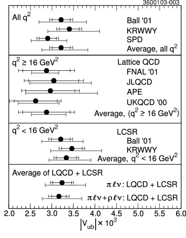
Figure 13: Values for $|V_{ub}|$ obtained from $\pi\ell\nu$ using the entire $q^{2}$ range for the various form-factor calculations (top block), using LQCD for $q^{2}\geq 16$ GeV² (second block), using LCSR for $q^{2}<16$ GeV² (third block), and our average of the last two (bottom block) for $\pi\ell\nu$ only and for $\pi\ell\nu$ and $\rho\ell\nu$ combined. In all cases, the top bar indicates the statistical and all the experimental systematics (combined in quadrature), the lower bar indicates the approximate “one standard deviation” range of motion due to the theoretical uncertainties.

VII.2 $|V_{ub}|$ from $B\to\rho\ell\nu$

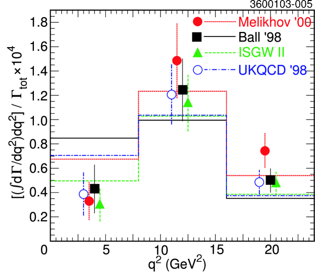
Figure 14: Measured branching fractions in the restricted $q^{2}$ intervals for $B^{0}\to\rho^{-}\ell^{+}\nu$ (points) and the best fit to the predicted $d\Gamma/dq^{2}$ (histograms) for the three models used to extract both rates and $|V_{ub}|$. The data points have small horizontal offsets introduced for clarity.

We proceed with $B\to\rho\ell\nu$ in much the same fashion as with $B\to\pi\ell\nu$. The fits of the different form factors to the rates extracted from the three $q^{2}$ intervals in the data are illustrated in Figure 14 and are summarized in Table 13. Because of the relatively large variation in the rates extracted from the data using the different form-factor calculations, we again perform the extraction of $|V_{ub}|$ entirely within the context of a given form-factor calculation. In general, the theoretical predictions do not match the data as well as we saw for the $\pi\ell\nu$ mode. In spite of some of the poor fits, we consider all four sets of form factors as we estimate $|V_{ub}|$ with this mode. As we expected from the branching fraction results, the $|V_{ub}|$ extracted from the $\rho\ell\nu$ information does not depend on the $\pi\ell\nu$ form factor used in the analysis.

Table 13: $|V_{ub}|$ extracted from fits to the rates measured in the three $q^{2}$ intervals for a variety of form factors for $\rho\ell\nu$. The table indicates form-factor calculation, $|V_{ub}|$ with statistical error only, predicted $\Gamma^{\text{th}}_{\rho}/|V_{ub}|^{2}$ with the estimated theoretical uncertainty, the $\chi^{2}$ for the fit, and the probability of $\chi^{2}$ given the two degrees of freedom.

$\pi$ Model	$\rho$ Model	$|V_{ub}|\times 10^{3}$	$\Gamma^{\text{th}}_{\rho}/|V_{ub}|^{2}$ (ps-1)	Fit $\chi^{2}$	$P(\chi^{2})$
Ball’01	Ball’98	$2.90\pm 0.21$	$16.9\pm 5.1$	7.6	0.02
Ball’01	ISGW2	$2.96\pm 0.21$	$14.2\pm 7.1$	3.3	0.19
Ball’01	Melikhov’00	$2.46\pm 0.17$	$26.2\pm 5.2$	8.1	0.02
Ball’01	UKQCD’98	$2.88\pm 0.20$	$16.5^{+3.5}_{-2.3}$	5.2	0.08
Ball’01	Ball’98	$2.90\pm 0.21$	$16.9\pm 5.1$	7.6	0.02
ISGW2	Ball’98	$2.90\pm 0.21$	$16.9\pm 5.1$	7.6	0.02
SPD	Ball’98	$2.90\pm 0.21$	$16.9\pm 5.1$	7.8	0.02

For an estimate of $|V_{ub}|$ based on the models and fits in Table 13, we take the Ball’98 results as the central value. Estimating the uncertainties as described in the previous section, we obtain

$$|V_{ub}|=(2.90\pm 0.21\;^{+0.31}_{-0.36}\;{}^{+0.73}_{-0.46})\times 10^{-3},$$ (12)

where the errors are statistical, experimental systematic, and the estimated uncertainties from 70% of the total spread in the results as we vary the $\rho\ell\nu$ form-factor calculations over $\pm 1$ standard deviation, respectively. This estimate is similar to, though somewhat larger than, that obtained from the quoted Ball’98 uncertainty.

Table 14: Values for $|V_{ub}|$ obtained using form factors (FF) from light-cone sum rules in the $q^{2}$ interval $0-16$ GeV² (first row) and from LQCD for $q^{2}\geq 16$ GeV² (second row). Only the statistical errors are indicated. The data rates obtained using Ball’01 for $\pi\ell\nu$ and Ball’98 for $\rho\ell\nu$ were used as the input for all values obtained.

$\rho$ FF	$|V_{ub}|\times 10^{3}$	$\Gamma^{\text{th}}_{\rho}/|V_{ub}|^{2}$ (ps-1)	Fit $\chi^{2}$	$P(\chi^{2})$
Ball’98	$2.67\pm 0.27$	$14.2\pm 4.3$	4.5	0.03
UKQCD’98	$3.34\pm 0.32$	$2.9^{+0.62}_{-0.40}$	–	–

Restricting ourselves to the theoretically more reliable use of LQCD for $q^{2}\geq 16$ GeV² and LCSR for $q^{2}<16$ GeV², we have only the two results listed in Table 14. In addition to the theoretical uncertainty quoted for UKQCD’98, we add an additional 20% in quadrature as an estimate of the quenching uncertainty. This is larger than for the $\pi\ell\nu$ case both because the $\rho$ is a broad resonance and because of the potential for larger biases from quenching given the interference between the various form factors. We also apply our reinterpretation of symmetrical theoretical errors on the rate as symmetric errors on the amplitude. The results in the two $q^{2}$ intervals are thus

$$|V_{ub}|_{q^{2}\geq 16\text{ GeV}^{2}}=(3.34\pm 0.32\;^{+0.27}_{-0.36}\;{}^{+0.50}_{-0.40})\times 10^{-3},$$ (13)

and

$$|V_{ub}|_{q^{2}<16\text{ GeV}^{2}}=(2.67\pm 0.27\;^{+0.38}_{-0.42}\;{}^{+0.47}_{-0.35})\times 10^{-3}.$$ (14)

We average the LQCD and LCSR results, with correlated experimental systematics taken into account. We again employ the procedure described in Appendix C. The optimal weight for combining the two intervals, treating the systematic uncertainties as completely correlated, is $\alpha_{\rho}=0.5$.

$$|V_{ub}|=(3.00\pm 0.21\;^{+0.29}_{-0.35}\;{}^{+0.49}_{-0.38}\pm 0.28)\times 10^{-3}.$$ (15)

The errors are statistical, experimental systematic, theoretical systematic based on the LQCD and LCSR uncertainties, and $\rho\ell\nu$ form-factor shape uncertainty. To be conservative, we have assigned the latter error based on the variation seen in the total branching fraction in this mode. The contribution from the $\pi\ell\nu$ form-factor shape is negligible. Again, we take this as our preferred method of extracting $|V_{ub}|$ from our $\rho\ell\nu$ data.

The $|V_{ub}|$ results obtained from $\rho\ell\nu$ are shown in Figure 15.

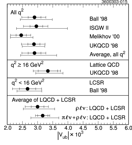
Figure 15: Values for $|V_{ub}|$ obtained from $\rho\ell\nu$ using the entire $q^{2}$ range for the various form-factor calculations (top block), using LQCD for $q^{2}\geq 16$ GeV² (second block), using LCSR for $q^{2}<16$ GeV² (third block), and our average of the last two (bottom block) for $\rho\ell\nu$ only and for $\pi\ell\nu$ and $\rho\ell\nu$ combined. In all cases, the top bar indicates the statistical and all the experimental systematics (combined in quadrature), the lower bar indicated the approximate “one standard deviation” range of motion due to the theoretical uncertainties.

VII.3 $|V_{ub}|$ from a Combination of $B\to\pi\ell\nu$ and $B\to\rho\ell\nu$

We have averaged the $|V_{ub}|$ determinations obtained separately from the $B\to\pi\ell\nu$ and $B\to\rho\ell\nu$ modes. For this average, we considered only the results obtained using the LCSR and LQCD calculations applied to the $q^{2}<16\ \textrm{GeV}^{2}$ and $q^{2}\geq 16\ \textrm{GeV}^{2}$ results, respectively. The averaging procedure amounts to the determination of the optimal weight $\beta$ to be applied to the LCSR and LQCD average obtained from $B\to\pi\ell\nu$ relative to that obtained from $B\to\rho\ell\nu$ (see Appendix C). We held the values $\alpha_{\pi}$ and $\alpha_{\rho}$, each of which determines the weight of the LQCD result relative to the LCSR result in the individual mode, fixed at the optimal values found in the preceding subsections. The weight $\beta=0.7$ provided the optimal combination. With this weighting, we find

$$|V_{ub}|=(3.17\pm 0.17\;^{+0.16}_{-0.17}\;{}^{+0.53}_{-0.39}\pm 0.03)\times 10^{-3}.$$ (16)

The errors are statistical, experimental systematic, theoretical systematic based on the LQCD and LCSR uncertainties, and $\rho\ell\nu$ form-factor shape uncertainty, respectively. Note that because of cross feed among the modes considered, the $\pi\ell\nu$ and $\rho\ell\nu$ modes are anticorrelated, resulting, in particular, in the minimal dependence of the average result on the $\rho\ell\nu$ form-factor shape.

VIII Summary

With a sample of $9.7\times 10^{6}$ $B\bar{B}$ pairs, we have studied $B$ decays to $\pi\ell\nu$, $\rho\ell\nu$, $\omega\ell\nu$, and $\eta\ell\nu$, where $\ell=e\text{ or }\mu$. From the combination of a broad momentum range for the charged lepton momentum and independent extraction of rates in three separate $q^{2}$ intervals, we were able to reduce the uncertainties from modeling within the form-factor calculations. For the decay $B^{0}\to\pi^{-}\ell^{+}\nu$, we have determined the branching fractions

$${\cal B}(0\leq q^{2}<8\,\text{GeV}^{2}) = (0.43\pm 0.11\pm 0.05\pm 0.004\pm 0.01)\times 10^{-4}$$ (17)

$${\cal B}(8\leq q^{2}<16\,\text{GeV}^{2}) = (0.65\pm 0.11\pm 0.07\pm 0.01\pm 0.03)\times 10^{-4}$$

$${\cal B}(q^{2}\geq 16\,\text{GeV}^{2}) = (0.25\pm 0.09\pm 0.04\pm 0.01\pm 0.03)\times 10^{-4}.$$

Combining these rates and taking into account correlated systematic uncertainties, we obtain

$${\cal B}(B^{0}\to\pi^{-}\ell^{+}\nu)=(1.33\pm 0.18\pm 0.11\pm 0.01\pm 0.07)\times 10^{-4},$$ (18)

where the errors are statistical, experimental systematic, the estimated uncertainties from the $\pi\ell\nu$ form factor, and those from the $\rho\ell\nu$ form factors, respectively.

For the decay $B^{0}\to\rho^{-}\ell^{+}\nu$, we have determined the branching fractions

$${\cal B}(0\leq q^{2}<8\,\text{GeV}^{2}) = (0.43\pm 0.20\pm 0.23\pm 0.09\pm 0.01)\times 10^{-4}$$ (19)

$${\cal B}(8\leq q^{2}<16\,\text{GeV}^{2}) = (1.24\pm 0.26\;^{+0.27}_{-0.33}\pm 0.22\pm 0.004)\times 10^{-4}$$

$${\cal B}(q^{2}\geq 16\,\text{GeV}^{2}) = (0.50\pm 0.10\;^{+0.08}_{-0.11}\pm 0.19\pm 0.004)\times 10^{-4}.$$

Combining these rates, again taking into account correlated systematic uncertainties, we obtain

$${\cal B}(B^{0}\to\rho^{-}\ell^{+}\nu)=(2.17\pm 0.34\;^{+0.47}_{-0.54}\pm 0.41\pm 0.01)\times 10^{-4},$$ (20)

where the errors are statistical, experimental systematic, the estimated uncertainties from the $\rho\ell\nu$ form factors, and those from the $\pi\ell\nu$ form factor, respectively.

When the theoretical uncertainties that result from form-factor $q^{2}$–dependence are evaluated in a common fashion, the branching fractions obtained in this analysis have uncertainties from the form-factor $q^{2}$–dependence that are reduced by about a factor of two compared to previous $\rho\ell\nu$ analyses bb:lkg_cleo_exclusive ; bb:lange_cleo_exclusive ; bb:newBabar . These uncertainties are almost eliminated for the $\pi\ell\nu$ branching fraction.

We see evidence for the decay $B^{+}\to\eta\ell^{+}\nu$ with a statistical significance corresponding roughly to $3.2\sigma$. The rate we obtain,

$${\cal B}(B^{+}\to\eta\ell^{+}\nu)=(0.84\pm 0.31\pm 0.16\pm 0.09)\times 10^{-4},$$ (21)

is consistent, within sizable errors, with that expected from the measured pion rate and isospin relations. Only an ISGW II form factor has been examined, and a 10% model dependence uncertainty has been assigned based on the previous CLEO $\pi\ell\nu$ analysis. The final error quoted combines this estimate with the dependence on the $\pi\ell\nu$ and $\rho\ell\nu$ form factors.

From the $\pi\ell\nu$ $q^{2}$ behavior that we have observed, we find the ISGW II form factor for $\pi\ell\nu$ consistent with data at only the 3% level.

By fitting LQCD and LCSR calculations to the observed $q^{2}$ behavior in $\pi\ell\nu$, restricting each calculation to its valid $q^{2}$ range, and then combining the results, we extract

$$|V_{ub}|=(3.24\pm 0.22\pm 0.13\;^{+0.55}_{-0.39}\pm 0.09)\times 10^{-3},$$ (22)

where the errors are statistical, experimental systematic, the estimated uncertainties from the $\pi\ell\nu$ form-factor shape and normalization, and those from the $\rho\ell\nu$ form factors’ shapes, respectively. From a similar analysis of the $\rho\ell\nu$ mode, we obtain

$$|V_{ub}|=(3.00\pm 0.21\;^{+0.29}_{-0.35}\;{}^{+0.49}_{-0.38}\pm 0.28)\times 10^{-3}.$$ (23)

The errors are statistical, experimental systematic, theoretical systematic based on the LQCD and LCSR uncertainties, and $\rho\ell\nu$ form-factor shape uncertainty, respectively. In general, the $\rho\ell\nu$ form-factor calculations did not agree as well with the observed $\rho\ell\nu$ data as did the $\pi\ell\nu$ form-factor calculations with the $\pi\ell\nu$ data.

Combining these two modes for an overall result from this analysis, we obtain

$$|V_{ub}|=(3.17\pm 0.17\;^{+0.16}_{-0.17}\;{}^{+0.53}_{-0.39}\pm 0.03)\times 10^{-3}.$$ (24)

Given the manner with which the theoretical uncertainties have been estimated, the quoted values should be interpreted as being closer in spirit to “one standard deviation” than to “the allowed range”.

These results trade off the potential statistical gain over the previous CLEO analyses in favor of relaxation of theoretical constraints. Had we fixed the relative rate in the three $q^{2}$ intervals in the $\pi\ell\nu$ and $\rho\ell\nu$ modes, a more pronounced improvement in statistical precision would have resulted. By relaxing the constraint, on the other hand, we have minimized our reliance on modeling in extraction of rates and of $|V_{ub}|$.

These results supersede the $\pi\ell\nu$ and $\rho\ell\nu$ results obtained in reference bb:lkg_cleo_exclusive . They agree, within measurement uncertainties, with the CLEO 2000 $\rho\ell\nu$ result bb:lange_cleo_exclusive and with the recent BABAR $\rho\ell\nu$ analysis bb:newBabar .

The results for $|V_{ub}|$ obtained here are compatible with the results obtained from the recent CLEO end-point measurement bb:new_endpoint . The estimated theoretical uncertainties remain sizable for both $\pi\ell\nu$ and $\rho\ell\nu$, and there remain uncertainties in the estimates themselves. We therefore do not average these results, but view the compatibility as an indication that the uncertainties have not been appreciably underestimated. Significant progress in extraction of $|V_{ub}|$ from exclusive decays will require a major improvement in theory.

We thank A. Kronfeld, J. Simone, T. Onogi, T. Feldmann, P. Kroll, C. Maynard, and D. Melikhov for assistance with form factors. We gratefully acknowledge the effort of the CESR staff in providing us with excellent luminosity and running conditions. M. Selen thanks the Research Corporation, and A.H. Mahmood thanks the Texas Advanced Research Program. This work was supported by the National Science Foundation and the U.S. Department of Energy.

Appendix A Description of experimental systematic uncertainty determination

The techniques employed in this analysis rest fundamentally on complete, accurate reconstruction of all particles from both $B$ decays in an event. As a result, systematic uncertainty estimates that reflect uncertainties in the detector simulation must account for the reliability with which an entire event can be reconstructed, not just the signal particles. For example, if there is a residual uncertainty in the track reconstruction efficiency, the signal efficiency will not only be affected by incorrectly assessing the loss of the signal mode particles, it will also be affected by “misreconstruction” of the neutrino four–momentum. Furthermore, the rate at which background samples can smear into the signal region is also affected by the overall misreconstruction.

We therefore estimate the systematic uncertainties due to detector modeling by modifying each reconstructed Monte Carlo event in each signal and background sample. For each study, the size of the variation has generally been determined by independent comparisons of data and Monte Carlo. The following list describes the variations that enter the systematic determination:

tracking efficiency

We have limited our uncertainty in track–finding efficiency for high (above 250 MeV/$c$) and low momentum tracks to be under 0.5% and 2.6%, respectively. These limits were obtained with hadronic samples, and therefore include any discrepancies in the interaction cross sections. To determine the systematic error from the uncertainty in tracking efficiency, we apply an additional inefficiency of 0.75% and 2.6% to each high momentum track and to each low momentum track, respectively, in the simulation.

tracking resolution

We increase the mismeasurement of each momentum component for each reconstructed charged particle by 10% of itself, which is outside the range for which core distributions agree, but compensates for discrepancies in the tails.

$\gamma$ efficiency

We have limited our uncertainty in photon reconstruction efficiency to 2%. In our studies, we have actually applied an additional 3% efficiency loss per photon, then scaled the observed shifts back by $2/3$.

$\gamma$ resolution

We also degrade the photon energy resolution by 10% of itself.

split-off simulation

Studies of $\gamma\gamma\to K_{S}K_{S}$ have indicated that the combination of mismodeling the physics processes and hadronic showers leads to an excess of isolated reconstructed showers (split offs) at the rate of $0.03$/hadron in data relative to the Monte Carlo. To estimate the potential effect on our analysis, we interpret the entire excess as mismodeling of the hadronic showers, and add showers at this rate to each of our Monte Carlo samples.

split-off rejection

We bias our neural net parameter, which is derived from the distribution of energy within the crystals in the shower relative to the primary impact point of a “parent” charged hadron, to move photon–like results in the Monte Carlo towards hadronic–shower–like results. We limit the variations based on data and Monte Carlo comparisons of the parameter as a function of shower energy.

$K_{L}$ showers

In our simulation of $K_{L}$ showers, we increase the energy deposited in our CsI calorimeter. The variation is based on data and Monte Carlo comparisons of the energy deposited by $K^{\pm}$ showers after correction for the minimum–ionizing component.

$K_{L}$ production

By comparing the data and Monte Carlo $K_{S}$ energy spectrum and yield, we found that our $K_{L}$ rate needed to be decreased by $(7.2\pm 1.0)$%, and that no correction was needed for the spectrum. The nominal analysis reweights events with $K_{L}$ accordingly, and we vary the weight according to its uncertainty to estimate the systematic contribution.

extra $\nu$ production

An important source of background is events that contain both a $b\to c\ell\nu$ decay and a $c\to s\ell\nu$ decay, where the latter can originate with either $B$ meson in the event. We reweight the Monte Carlo so that the lepton momentum spectrum from secondary charm decay agrees with a spectrum obtained by convoluting a recent measurement of the charm meson momentum spectrum from $B$ decay bb:moneti with the MARK III measurement of the inclusive lepton momentum spectrum from charm decay bb:Delco . The nominal result is corrected based on this procedure. To estimate the systematic uncertainty, we define spectrum “envelopes” and reweight our Monte Carlo samples to match this spectrum. The envelopes were defined by throwing 500 toy Monte Carlo spectra in which all experimental inputs were varied according to their uncertainties and finding the variation within each momentum bin that contained 68% of the toy spectra.

particle ID

We simultaneously shift all dE/dx and time-of-flight distributions in the simulation by 1/4 and 1/2 of the intrinsic resolution, respectively. We take the full variation we observe as our uncertainty, even though this procedure leads to a very conservative systematic estimate.

For each of these variations, we modify or reweight each event in each Monte Carlo sample in a full reanalysis of these samples. The set of modified samples for each variation replaces the nominal samples input to the branching fraction fit. For each variation, the shifts in the fit results provide the first input into the systematic estimates on the branching fractions for that variation. We can view the shifts in results as arising from two components: a change in the signal efficiency and a change in the predicted background level. These changes tend to cancel in the total shift: a variation that reduces the signal reconstruction efficiency also simultaneously increases the background level (and reduces the signal yield from the fit). As the main text describes, we increase our systematic estimate to allow for imperfections in the predicted cancellation.

Appendix B Extraction of $|V_{ub}|$ from the measured $d\Gamma(B^{0}\to\pi^{-}\ell^{+}\nu)/dq^{2}$ data with future form-factor calculations

The branching fractions in the three $q^{2}$ ranges for $B\to\pi\ell\nu$ exhibit very little dependence on the precise form factors used to extract the branching fractions. The results can therefore be reliably used to obtain values for $|V_{ub}|$ using future $B\to\pi\ell\nu$ form-factor calculations that are improved over those used in this paper. This appendix provides the detail needed to ascertain the proper experimental uncertainties for such an extraction using the same fitting technique presented above. The main difficulty stems from proper evaluation of the experimental uncertainties because of correlations (both positive and negative) among the results for the three ranges. The correlations arise both statistically from the fitting procedure used to extract the three rates and systematically as we vary the details of the simulation.

Table 15: Central values and statistical uncertainties for $B^{0}\to\pi^{-}\ell^{+}\nu$ branching fractions for the nominal fit and for each systematic variation of the Monte Carlo samples input to the fit. The detector–related systematic uncertainties in $|V_{ub}|$ are obtained by fitting the results from the relevant set of $q^{2}$ intervals for each systematic study. The total branching fraction is shown as well for completeness. All results were obtained using the Ball’01 form factor for the $\pi\ell\nu$ modes and the Ball’98 form factors for the $\rho\ell\nu$ modes.

systematic	$10^{4}\times\mathcal{B}(B^{0}\to\pi^{-}\ell^{+}\nu)$
change	total	$0\leq q^{2}<8\,\text{GeV}^{2}$	$8\leq q^{2}<16\,\text{GeV}^{2}$	$16\,\text{GeV}^{2}\leq q^{2}<q^{2}_{\mathrm{max}}$
nominal	$1.327\pm 0.177$	$0.431\pm 0.106$	$0.651\pm 0.105$	$0.245\pm 0.094$
$\gamma$ eff.	$1.348\pm 0.194$	$0.476\pm 0.117$	$0.674\pm 0.117$	$0.198\pm 0.103$
$\gamma$ resol.	$1.379\pm 0.183$	$0.445\pm 0.111$	$0.686\pm 0.109$	$0.249\pm 0.096$
$K_{L}$ shower	$1.311\pm 0.173$	$0.426\pm 0.104$	$0.642\pm 0.104$	$0.242\pm 0.091$
particle ID	$1.342\pm 0.180$	$0.414\pm 0.108$	$0.668\pm 0.107$	$0.260\pm 0.096$
split-off rejection	$1.338\pm 0.179$	$0.415\pm 0.108$	$0.667\pm 0.107$	$0.255\pm 0.095$
track eff.	$1.357\pm 0.185$	$0.446\pm 0.112$	$0.669\pm 0.110$	$0.242\pm 0.097$
track resol.	$1.317\pm 0.179$	$0.438\pm 0.108$	$0.664\pm 0.108$	$0.215\pm 0.094$
split-off sim.	$1.326\pm 0.178$	$0.432\pm 0.108$	$0.655\pm 0.106$	$0.240\pm 0.093$
$K_{L}$ production $\uparrow$	$1.325\pm 0.176$	$0.431\pm 0.106$	$0.651\pm 0.105$	$0.244\pm 0.094$
$K_{L}$ production $\downarrow$	$1.330\pm 0.177$	$0.432\pm 0.107$	$0.653\pm 0.105$	$0.246\pm 0.094$
$\nu$ production $\uparrow$	$1.344\pm 0.178$	$0.425\pm 0.106$	$0.669\pm 0.106$	$0.251\pm 0.095$
$\nu$ production $\downarrow$	$1.322\pm 0.175$	$0.439\pm 0.106$	$0.641\pm 0.104$	$0.242\pm 0.093$

To extract a central value of $|V_{ub}|$, we perform a $\chi^{2}$ fit to the nominal branching fractions from the three $q^{2}$ intervals listed in Table 15. This $|V_{ub}|$ fit includes the correlation coefficients among the rates from the branching fraction fit to the data: $\rho_{12}=-0.035$, $\rho_{13}=0.003$, and $\rho_{23}=-0.037$.

To evaluate the error arising from simulation uncertainties (“$\nu$ simulation” in Table 4) on the results, we redo our $\chi^{2}$ fit for $|V_{ub}|$ using the new rates listed in Table 15 for each variation. For the results presented here, we have used the correlation coefficients from the branching fraction fit to the data for each variation. In practice, the coefficients remain stable enough that using the nominal coefficients in all fits is sufficient. The change relative to the nominal $|V_{ub}|$ result provides the first input to the uncertainty estimate. For the uncertainty estimate in $K_{L}$ production and secondary $\nu$ production, we take the average of the “up” and “down” shifts as our overall estimate. To allow for misestimation of correlated changes between background levels and signal efficiencies in the results (see main text), we increase the fractional uncertainty on $|V_{ub}|$ from each variation by adding in quadrature the quantities listed in Table 16. Finally, the $\gamma$ efficiency uncertainty should be scaled back to $2/3$ of the value found above. We combine all of the uncertainties in quadrature to arrive at the total “$\nu$ simulation” systematic for $|V_{ub}|$.

Table 16: Fractional uncertainties to be added in quadrature to systematic shifts in $|V_{ub}|$ to account for uncertainty in cancellations arising from correlated efficiency and background changes. The correction is shown for the various different $q^{2}$ ranges used in this analysis.

systematic	additional systematic (%)
change	full range	$0\leq q^{2}<16\,\text{GeV}^{2}$	$0\leq q^{2}<8\,\text{GeV}^{2}$	$8\leq q^{2}<16\,\text{GeV}^{2}$	$16\,\text{GeV}^{2}\leq q^{2}<q^{2}_{\mathrm{max}}$
$\gamma$ eff.	1.67	0.51	0.72	1.22	1.49
$\gamma$ resol.	0.19	0.28	0.14	0.43	0.30
$K_{L}$ shower	0.25	0.30	0.14	0.16	0.46
particle ID	0.25	1.09	0.29	0.27	0.58
split-off rejection	0.00	0.56	0.24	0.21	0.35
track eff.	0.99	1.62	0.72	0.90	1.17
track resol.	0.49	0.25	0.14	0.11	0.44
split-off sim.	0.23	0.39	0.24	0.11	0.17
$K_{L}$ production	0.01	0.02	0.01	0.00	0.01
$\nu$ production	0.12	0.43	0.28	0.19	0.13

We evaluate the uncertainty from our modeling of the $B\to X_{u}\ell\nu$ backgrounds in much the same fashion. The fit variations that we have used for this purpose are listed in Table 17. An earlier version of our $B\to X_{u}\ell\nu$ generator was used in the study, and the table also shows the “nominal” result obtained with that version. We did not expect large differences from our change, and indeed the results obtained are very similar to the nominal results in Table 15. To obtain the uncertainty estimate resulting from the hadronization model, we compare the results using purely nonresonant hadronization to that using our nominal mixture of resonant and nonresonant modes. To obtain the uncertainty resulting from our choice of parameters for the OPE-based inclusive differential rate calculation, we take the average of the shift from the last two lines in the table relative to the above nonresonant result. Note that these variations do not affect our signal Monte Carlo samples.

Table 17: Central values and statistical uncertainties for $B^{0}\to\pi^{-}\ell^{+}\nu$ branching fractions for the reference fit and for each systematic variation of the $B\to X_{u}\ell\nu$ background simulation input to the fit. The associated systematic uncertainties in $|V_{ub}|$ are obtained by fitting the results from the relevant set of $q^{2}$ intervals for each systematic study. The total branching fraction is shown as well for completeness. All results were obtained using the Ball’01 form factor for the $\pi\ell\nu$ modes and the Ball’98 form factors for the $\rho\ell\nu$ modes.

OPE	hadron-	$10^{4}\times\mathcal{B}(B^{0}\to\pi^{-}\ell^{+}\nu)$
parameters	ization	total	$0\leq q^{2}<8\,\text{GeV}^{2}$	$8\leq q^{2}<16\,\text{GeV}^{2}$	$16\,\text{GeV}^{2}\leq q^{2}<q^{2}_{\mathrm{max}}$
nominal	nominal	$1.324\pm 0.177$	$0.423\pm 0.107$	$0.655\pm 0.105$	$0.246\pm 0.094$
nominal	nonres.	$1.322\pm 0.177$	$0.431\pm 0.106$	$0.639\pm 0.105$	$0.251\pm 0.094$
“High”	nonres.	$1.311\pm 0.176$	$0.428\pm 0.106$	$0.637\pm 0.105$	$0.246\pm 0.094$
“Low”	nonres.	$1.329\pm 0.177$	$0.434\pm 0.106$	$0.646\pm 0.105$	$0.248\pm 0.095$

For the remainder of the systematic uncertainties, we take one half of the fractional uncertainties listed in Table 4. The factor of one half arises because of the square root involved in extraction of $|V_{ub}|$ from the rates.

Appendix C Averaging $|V_{ub}|$ results

In each of the $\pi\ell\nu$ and $\rho\ell\nu$ modes, we have extracted two results for $|V_{ub}|$ that are largely free from modeling assumptions: a value based on the application of LCSR–derived form factors for $q^{2}<16\ \textrm{GeV}^{2}$, and a value based on the application of LQCD–derived form factors for $q^{2}\geq 16\ \textrm{GeV}^{2}$. We therefore have three averages to be calculated: the combination of the two results within the $\pi\ell\nu$ mode and within the $\rho\ell\nu$ mode, and the combination of the two modes. The averaging procedure should take into account, in particular, the correlations present in the systematic uncertainties in the result. This appendix describes our averaging procedure.

The statistical correlations have been taken into account in the LCSR–derived results. An evaluation of remaining statistical correlations found that they had little impact on the final statistical error, and we have not included them in the final procedure. Proper treatment would have led to a decrease in the overall uncertainty that would be hidden at the quoted precision.

Regarding theoretical uncertainties, while the two techniques have different systematic effects, both approaches currently have systematic issues that are difficult to evaluate. For example, there is a quark–hadron duality assumption in the LCSR approach, and the current LQCD calculations have been evaluated in the “quenched” approximation. Treating the uncertainties as uncorrelated would therefore be likely to underestimate the “true” theoretical uncertainty. To be conservative, we treat the theoretical uncertainties as if they were fully correlated.

Let us first consider the two results obtained within a given mode. We wish to combine the results with a weight that minimizes the overall uncertainty and preserves the systematic correlation information. Defining the weight of the LQCD–derived result (denoted $|V_{ub}|^{\geq 16}$) by $\alpha$, the LCSR–derived result (denoted $|V_{ub}|^{<16}$) enters with a weight $1-\alpha$:

$$|V_{ub}|_{\alpha}=\alpha|V_{ub}|^{\geq 16}+(1-\alpha)|V_{ub}|^{<16}.$$ (25)

The statistical uncertainties are uncorrelated, and are combined as

$$\sigma_{\mathrm{stat}}^{2}=(\alpha\sigma_{\mathrm{stat}}^{\geq 16})^{2}+((1-\alpha)\sigma_{\mathrm{stat}}^{<16})^{2}.$$ (26)

Correlated uncertainties, such as the theoretical uncertainties, are combined as

$$\sigma_{\mathrm{corr}}=(\alpha\sigma_{\mathrm{corr}}^{\geq 16})+((1-\alpha)\sigma_{\mathrm{corr}}^{<16}).$$ (27)

For each simulation variation (labelled $i$), we perform the full analysis to obtain $|V_{ub}|^{\geq 16}_{i}$) and $|V_{ub}|^{<16}_{i}$. The systematic uncertainty defined for the variation is

$$\sigma_{i}=|V_{ub}|_{\alpha}^{\mathrm{nom}}-(\alpha|V_{ub}|^{\geq 16}_{i}+(1-\alpha)|V_{ub}|^{<16}_{i}),$$ (28)

where $|V_{ub}|_{\alpha}^{\mathrm{nom}}$ is the average resulting from Equation 25. This procedure preserves the systematic correlation. We combine this estimate in quadrature with the additional uncertainty contribution to allow for imperfect modeling of the correlated changes between signal efficiency and raw yield (see Section V).

Finally, for each value of $\alpha$ the experimental and theoretical uncertainties are combined in quadrature (taking the average theoretical uncertainty in the case of asymmetric uncertainties). We scan over $\alpha$ and choose the value that minimizes the total uncertainty.

We perform a similar procedure to combine the results from the two modes. The weights obtained individually for the different $q^{2}$ regions in each mode are fixed. The uncorrelated, correlated, and anticorrelated uncertainties are combined in exact analogy to the above descriptions. Taking $\beta$ as the weight of the $\pi\ell\nu$ mode in the average, we have

$$|V_{ub}|_{\beta}=\beta|V_{ub}|^{\pi}+(1-\beta)|V_{ub}|^{\rho}.$$ (29)

For each simulation variation, the systematic estimate becomes

$$\sigma_{i}=|V_{ub}|_{\beta}^{\mathrm{nom}}-\left[\beta(\alpha_{\pi}|V_{ub}|^{\geq 16,\pi}_{i}+(1-\alpha_{\pi})|V_{ub}|^{<16,\pi}_{i})+(1-\beta)(\alpha_{\rho}|V_{ub}|^{\geq 16,\rho}_{i}+(1-\alpha_{\rho})|V_{ub}|^{<16,\rho}_{i})\right].$$ (30)

These uncertainties are, as before, combined in quadrature, along with the contribution for imperfect modeling of the correlated efficiency and yield changes.

We scan over the weight $\beta$ to find the value that minimizes the overall combined uncertainty. Once again we treat the theoretical uncertainties in the $\pi\ell\nu$ and $\rho\ell\nu$ form factors as correlated in this procedure.

References

- (1) N. Cabibbo, Phys. Rev. Lett. 10, 531 (1963); M. Kobayashi and T. Maskawa, Prog. Theor. Phys. 49, 652 (1973).
- (2) M. Battaglia and L. Gibbons, Determination of , in Review of Particle Properties, K. Hagiwara et al., Phys. Rev. D 66, 010001 (2002).
- (3) J. P. Alexander et al. [CLEO Collaboration], Phys. Rev. Lett. 77, 5000 (1996).
- (4) B. H. Behrens et al. [CLEO Collaboration], Phys. Rev. D 61, 052001 (2000) [arXiv:hep-ex/9905056].
- (5) V. Boisvert, Ph. D. Thesis, Cornell University, 2002 (unpublished).
- (6) A. Abada et al., Nucl. Phys. B 416, 675 (1994) [arXiv:hep-lat/9308007].
- (7) C. R. Allton et al. [APE Collaboration], Phys. Lett. B 345, 513 (1995) [arXiv:hep-lat/9411011].
- (8) L. Del Debbio, J. M. Flynn, L. Lellouch, and J. Nieves [UKQCD Collaboration], Phys. Lett. B 416, 392 (1998) [arXiv:hep-lat/9708008].
- (9) S. Hashimoto, K. I. Ishikawa, H. Matsufuru, T. Onogi, and N. Yamada, Phys. Rev. D 58, 014502 (1998) [arXiv:hep-lat/9711031].
- (10) S. Ryan, A. El-Khadra, S. Hashimoto, A. Kronfeld, P. B. Mackenzie, and J. Simone, Nucl. Phys. Proc. Suppl. 73, 390 (1999) [arXiv:hep-lat/9810041].
- (11) S. M. Ryan, A. X. El-Khadra, A. S. Kronfeld, P. B. Mackenzie, and J. N. Simone, Nucl. Phys. Proc. Suppl. 83, 328 (2000) [arXiv:hep-lat/9910010].
- (12) L. Lellouch, [arXiv:hep-ph/9912353].
- (13) K. C. Bowler et al. [UKQCD Collaboration], Phys. Lett. B 486, 111 (2000) [arXiv:hep-lat/9911011].
- (14) D. Becirevic and A. B. Kaidalov, Phys. Lett. B 478, 417 (2000) [arXiv:hep-ph/9904490].
- (15) S. Aoki et al. [JLQCD Collaboration], Nucl. Phys. Proc. Suppl. 94, 329 (2001) [arXiv:hep-lat/0011008].
- (16) A. X. El-Khadra, A. S. Kronfeld, P. B. Mackenzie, S. M. Ryan, and J. N. Simone, Phys. Rev. D 64, 014502 (2001) [arXiv:hep-ph/0101023].
- (17) S. Aoki et al. [JLQCD Collaboration], Phys. Rev. D 64, 114505 (2001) [arXiv:hep-lat/0106024].
- (18) A. Abada, D. Becirevic, P. Boucaud, J. P. Leroy, V. Lubicz, and F. Mescia, Nucl. Phys. B 619, 565 (2001) [arXiv:hep-lat/0011065].
- (19) P. Ball and V. M. Braun, Phys. Rev. D 55, 5561 (1997) [arXiv:hep-ph/9701238].
- (20) P. Ball and V. M. Braun, Phys. Rev. D 58, 094016 (1998) [arXiv:hep-ph/9805422].
- (21) A. Khodjamirian, R. Rückl, S. Weinzierl, and O. I. Yakovlev, Phys. Lett. B 410, 275 (1997) [arXiv:hep-ph/9706303].
- (22) A. Khodjamirian, R. Rückl, S. Weinzierl, C. W. Winhart, and O. I. Yakovlev, Phys. Rev. D 62, 114002 (2000) [arXiv:hep-ph/0001297].
- (23) A. P. Bakulev, S. V. Mikhailov, and R. Ruskov, [arXiv:hep-ph/0006216].
- (24) T. Huang, Z. Li, and X. Wu, [arXiv:hep-ph/0011161].
- (25) W. Y. Wang and Y. L. Wu, Phys. Lett. B 515, 57 (2001) [arXiv:hep-ph/0105154].
- (26) W. Y. Wang and Y. L. Wu, Phys. Lett. B 519, 219 (2001) [arXiv:hep-ph/0106208].
- (27) P. Ball and R. Zwicky, JHEP 0110, 019 (2001) [arXiv:hep-ph/0110115].
- (28) M. Wirbel, B. Stech, and M. Bauer, Z. Phys. C 29, 637 (1985).
- (29) J. G. Körner and G. A. Schuler, Z. Phys. C 38, 511 (1988) [Erratum-ibid. C 41, 690 (1988)].
- (30) N. Isgur, D. Scora, B. Grinstein, and M. B. Wise, Phys. Rev. D 39, 799 (1989).
- (31) D. Scora and N. Isgur, Phys. Rev. D 52, 2783 (1995) [arXiv:hep-ph/9503486].
- (32) D. Melikhov, Phys. Rev. D 53, 2460 (1996) [arXiv:hep-ph/9509268].
- (33) M. Beyer and D. Melikhov, Phys. Lett. B 436, 344 (1998) [arXiv:hep-ph/9807223].
- (34) R. N. Faustov, V. O. Galkin, and A. Y. Mishurov, Phys. Rev. D 53, 6302 (1996) [arXiv:hep-ph/9508262].
- (35) N. B. Demchuk, P. Y. Kulikov, I. M. Narodetsky, and P. J. O’Donnell, Phys. Atom. Nucl. 60, 1292 (1997) [Yad. Fiz. 60N8, 1429 (1997)] [arXiv:hep-ph/9701388].
- (36) I. L. Grach, I. M. Narodetsky, and S. Simula, Phys. Lett. B 385, 317 (1996) [arXiv:hep-ph/9605349]. published.
- (37) Riazuddin, T. A. Al-Aithan, and A. H. Gilani, Int. J. Mod. Phys. A17, 4927 (2002) [arXiv:hep-ph/0007164].
- (38) D. Melikhov and B. Stech, Phys. Rev. D 62, 014006 (2000) [arXiv:hep-ph/0001113].
- (39) T. Feldmann and P. Kroll, Eur. Phys. J. C 12, 99 (2000) [arXiv:hep-ph/9905343].
- (40) J. M. Flynn and J. Nieves, Phys. Lett. B 505, 82 (2001) [arXiv:hep-ph/0007263].
- (41) M. Beneke and T. Feldmann, Nucl. Phys. B 592, 3 (2001) [arXiv:hep-ph/0008255].
- (42) H. M. Choi and C. R. Ji, Phys. Lett. B 460, 461 (1999) [arXiv:hep-ph/9903496].
- (43) T. Kurimoto, H.-n. Li, and A. I. Sanda, Phys. Rev. D 65, 014007 (2002) [arXiv:hep-ph/0105003].
- (44) Z. Ligeti and M. B. Wise, Phys. Rev. D 53, 4937 (1996) [arXiv:hep-ph/9512225].
- (45) E. M. Aitala et al. [E791 Collaboration], Phys. Rev. Lett. 80, 1393 (1998) [arXiv:hep-ph/9710216].
- (46) G. Burdman and J. Kambor, Phys. Rev. D 55, 2817 (1997) [arXiv:hep-ph/9602353].
- (47) L. Lellouch, Nucl. Phys. B 479, 353 (1996) [arXiv:hep-ph/9509358].
- (48) T. Mannel and B. Postler, Nucl. Phys. B 535, 372 (1998) [arXiv:hep-ph/9805425].
- (49) Y. Kubota et al., Nucl. Instrum. Methods Phys. Res., Sect. A 320, 66 (1992).
- (50) T. S. Hill, Nucl. Instrum. Methods Phys. Res., Sect. A 418, 32 (1998).
- (51) Spurious CsI showers from hadronic interactions add linearly to , but tend to average out in the vector sum for . Incorrect mass assignment also smears .
- (52) G. C. Fox and S. Wolfram, Phys. Rev. Lett. 41, 1581 (1978).
- (53) R. Brun et al., GEANT 3.15, CERN DD/EE/84-1.
- (54) F. De Fazio and M. Neubert, JHEP 9906, 017 (1999) [arXiv:hep-ph/9905351]
- (55) A. L. Kagan and M. Neubert, Eur. Phys. J. C7, 5 (1999) [arXiv:hep-ph/9805303].
- (56) S. Chen et al. [CLEO Collaboration], Phys. Rev. Lett. 87, 251807 (2001) [arXiv:hep-ex/0108032].
- (57) A. Bornheim et al. [CLEO Collaboration], Phys. Rev. Lett. 88, 231803 (2002) [arXiv:hep-ex/0202019].
- (58) K. Hagiwara et al. [Particle Data Group], Phys. Rev. D 66, 010001 (2002).
- (59) R. J. Barlow and C. Beeston, Comput. Phys. Commun. 77, 219 (1993).
- (60) T. Sjöstrand, [arXiv:hep-ph/9508391].
- (61) J. P. Alexander et al. [CLEO collaboration], Phys. Rev. Lett. 86, 2737 (2001) [arXiv:hep-ex/0006002].
- (62) J. L. Diaz-Cruz, G. Lopez Castro, and J. H. Munoz, Phys. Rev. D 54, 2388 (1996) [arXiv:hep-ph/9605344].
- (63) B. Aubert et al. [BABAR Collaboration], [arXiv:hep-ex/0301001]. Submitted to PRL.
- (64) L. Gibbons et al. [CLEO Collaboration], Phys. Rev. D 56, 3783 (1997) [arXiv:hep-ex/9703006].
- (65) R. M. Baltrusaitis et al. [MARK-III Collaboration], Phys. Rev. Lett. 54, 1976 (1985) [Erratum-ibid. 55, 638 (1985)].