The BABAR Collaboration

Search for $D^{0}$-$\kern 1.99997pt\overline{\kern-1.99997ptD}{}^{0}$ Mixing and a Measurement of the Doubly Cabibbo-suppressed Decay Rate in $D^{0}\rightarrow K\pi$ Decays

Abstract

We present results of a search for $D^{0}$-$\kern 1.99997pt\overline{\kern-1.99997ptD}{}^{0}$ mixing and a measurement of $R_{\rm D}$, the ratio of doubly Cabibbo-suppressed decays to Cabibbo-favored decays, based on an analysis of $D^{0}\rightarrow K^{+}\pi^{-}$ decays in 57.1 $\mbox{\,fb}^{-1}$ of data collected at or just below the $\mathchar 28935\relax{(4S)}$ resonance with the BABAR detector at the PEP-II collider. Our results are compatible with no mixing and no $C\!P$ violation. At the 95% confidence level, allowing for $C\!P$ violation, we find the mixing parameters ${x^{\prime}}^{2}<0.0022$ and $-0.056<y^{\prime}<0.039$, and the mixing rate $R_{\rm M}<0.16\%$. In the limit of no mixing, $R_{\rm D}=(0.357\pm 0.022\hbox{ (stat.)}\pm 0.027\hbox{ (syst.)})\%$ and the $C\!P$-violating asymmetry $A_{\rm D}=0.095\pm 0.061\hbox{ (stat.)}\pm 0.083\hbox{ (syst.)}$.

Within the Standard Model the level of $D^{0}$-$\kern 1.99997pt\overline{\kern-1.99997ptD}{}^{0}$ mixing is predicted to be below the sensitivity of current experiments Falk et al. (2002). For this reason $D^{0}$-$\kern 1.99997pt\overline{\kern-1.99997ptD}{}^{0}$ mixing is a good place to look for signals of new physics beyond the Standard Model Nelson (1999). Because new physics may not conserve $C\!P$, it is important to consider $C\!P$ violation when measuring mixing. Observation of $C\!P$ violation in $D^{0}$-$\kern 1.99997pt\overline{\kern-1.99997ptD}{}^{0}$ mixing would be an unambiguous sign of new physics Falk et al. (2002); Blaylock et al. (1995).

Mixing can be characterized by the two parameters $x\equiv\Delta m/\Gamma$ and $y\equiv\Delta\Gamma/2\Gamma$, where $\Delta m=m_{1}-m_{2}$ ($\Delta\Gamma=\Gamma_{1}-\Gamma_{2}$) is the difference in mass (width) between the two mass eigenstates and $\Gamma$ is the average width.

The dominant two-body decay of the $D^{0}$ is the right-sign (RS) Cabibbo-favored (CF) decay $D^{0}\rightarrow K^{-}\pi^{+}$. Evidence for mixing and $C\!P$ violation, if present, will appear in the wrong-sign (WS) decay $D^{0}\rightarrow K^{+}\pi^{-}$. Charge conjugates are implied unless otherwise stated. Two amplitudes contribute to the production of this final state: the tree-level amplitude for doubly Cabibbo-suppressed (DCS) decay of the $D^{0}$, and an amplitude for mixing followed by CF decay of the $\kern 1.99997pt\overline{\kern-1.99997ptD}{}^{0}$. Assuming that $x$, $y\ll 1$ and $C\!P$ is conserved, and with the convention $\Delta\Gamma=\Gamma(C\!P=+1)-\Gamma(C\!P=-1)$, the time-dependent, WS decay rate $T_{\rm WS}(t)$ for $D^{0}\rightarrow K^{+}\pi^{-}$ can be approximately Godang et al. (2000) related to the RS decay rate $T_{\rm RS}(t)$ by

$$T_{\rm WS}(t)=T_{\rm RS}(t)\left(R_{\rm D}+\sqrt{R_{\rm D}}y^{\prime}\;t+\frac{{x^{\prime}}^{2}+{y^{\prime}}^{2}}{4}t^{2}\right).$$ (1)

In Eq. (1), $t$ is the proper time of the $D^{0}$ decay measured in units of the $D^{0}$ lifetime $\tau_{D^{0}}$, $T_{\rm RS}(t)\propto e^{-t}$, $R_{\rm D}$ is the time-integrated rate of the direct DCS decay $D^{0}\rightarrow K^{+}\pi^{-}$ relative to the RS decay, and $x^{\prime}$, $y^{\prime}$ are related to $x$, $y$ by $x^{\prime}=x\cos\delta_{K\pi}+y\sin\delta_{K\pi}$ and $y^{\prime}=-x\sin\delta_{K\pi}+y\cos\delta_{K\pi}$, where $\delta_{K\pi}$ is the relative strong phase between the CF and DCS amplitudes. Physics beyond the Standard Model may include additional phases that are not $C\!P$-conserving. Such terms can be absorbed into a phase $\varphi$, described below. The time-integrated WS decay rate is

$$R_{\rm WS}=R_{\rm D}+\sqrt{R_{\rm D}}y^{\prime}+\frac{{x^{\prime}}^{2}+{y^{\prime}}^{2}}{2}\;.$$ (2)

Previous experiments have searched for mixing using wrong-sign hadronic Anjos et al. (1988); Aitala et al. (1998); Godang et al. (2000) and semileptonic Aitala et al. (1999) $D^{0}$ decays, or have searched for width differences between $C\!P=+1$ and $C\!P=-1$ states directly Link et al. (2000); Csorna et al. (2002); Abe et al. (2002). Since $x^{\prime}$ appears only quadratically in Eq. (1), its sign cannot be determined in an analysis based on the WS decay alone.

To allow for $C\!P$ violation, we apply Eq. (1) to $D^{0}$ and $\kern 1.99997pt\overline{\kern-1.99997ptD}{}^{0}$ separately. We determine {$R_{\rm WS}^{+}$, ${x^{\prime+}}^{2}$, $y^{\prime+}$} for $D^{0}$ candidates and {$R_{\rm WS}^{-}$, ${x^{\prime-}}^{2}$, $y^{\prime-}$} for $\kern 1.99997pt\overline{\kern-1.99997ptD}{}^{0}$ candidates. The separate $D^{0}$ and $\kern 1.99997pt\overline{\kern-1.99997ptD}{}^{0}$ results can be combined to form the quantities

$$A_{\rm D}=\frac{R_{\rm D}^{+}-R_{\rm D}^{-}}{R_{\rm D}^{+}+R_{\rm D}^{-}}\hbox{,\qquad}A_{\rm M}=\frac{R_{\rm M}^{+}-R_{\rm M}^{-}}{R_{\rm M}^{+}+R_{\rm M}^{-}}\;,$$ (3)

where $R_{\rm M}^{\pm}\equiv({x^{\prime\pm}}^{2}+{y^{\prime\pm}}^{2})/2$. $A_{\rm D}$ and $A_{\rm M}$ are related to $C\!P$ violation in the DCS decay and mixing amplitudes, respectively. $C\!P$ violation in the interference of DCS decay and mixing is parameterized by the phase $\varphi$:

$${x^{\prime}}^{\pm} = \sqrt[4]{\frac{1\pm A_{\rm M}}{1\mp A_{\rm M}}}(x^{\prime}\cos\varphi\pm y^{\prime}\sin\varphi),$$ (4)

$${y^{\prime}}^{\pm} = \sqrt[4]{\frac{1\pm A_{\rm M}}{1\mp A_{\rm M}}}(y^{\prime}\cos\varphi\mp x^{\prime}\sin\varphi).$$ (5)

An offset in $\varphi$ of $\pm\pi$ can be absorbed by a change in sign of both $x^{\prime}$ and $y^{\prime}$, effectively swapping the definition of the two physical $D^{0}$ states without any other observable consequence. To avoid this ambiguity, we use the convention that $|\varphi|<\pi/2$.

We select a very clean sample of RS and WS decays and fit for signal and background components in a $57.1~{}\mbox{\,fb}^{-1}$ dataset collected with the BABAR detector Aubert et al. (2002) at the PEP-II $e^{+}e^{-}$ storage ring. We extract the parameters describing mixing and DCS amplitudes from the WS decay-time distribution. To avoid potential bias, we finalized our data selection criteria and the procedures for fitting and extracting the statistical limits without examining the mixing results.

We select $D^{0}$ candidates from reconstructed $D^{*+}\rightarrow D^{0}\pi^{+}$ decays; this provides a clean sample of $D^{0}$ decays, and the charge of the pion (the ‘tagging pion’) identifies the production flavor of the neutral $D$. We retain each RS and WS $D^{0}$ candidate whose invariant mass $m_{K\pi}$ is within $60$ ${\mathrm{\,Me\kern-1.00006ptV\!/}c^{2}}$ of the $D^{0}$ mass. We require the mass difference $\delta m$ between the $D^{*+}$ and the $D^{0}$ candidate to be less than $m_{\pi}+25$ ${\mathrm{\,Me\kern-1.00006ptV\!/}c^{2}}$. Only $D^{*+}$ candidates with center-of-mass momenta above $2.6$ ${\mathrm{\,Ge\kern-1.00006ptV\!/}c}$ are retained, thereby rejecting $D^{*+}$ candidates from $B$ decays.

We determine the $D^{0}$ vertex by requiring that the $D^{0}$ decay tracks originate from a common point with a probability $p(\chi^{2})>1\%$, and then determine the $D^{*+}$ vertex by extrapolating the $D^{0}$ flight path back to the beam-beam interaction region. This procedure benefits from the small vertical size ($\approx 7$ $\mu$m) of the luminous region and the well-measured $D^{0}$ decay products. We constrain the trajectory of the tagging pion to originate from the $D^{*+}$ vertex, thus improving the measurement of $\delta m$. We then calculate the proper time $t$ of the $D^{0}$ decay from the dot product of the $D^{0}$ momentum vector and flight vector, defined by the $D^{*+}$ and $D^{0}$ decay vertices in three dimensions. The typical resolution is 0.2 ps.

We determine the mixing parameters by unbinned, extended maximum-likelihood fits to the RS and WS samples simultaneously. We perform four separate fit cases: first, a general fit allowing for possible $C\!P$ violation, which treats WS $D^{0}$ and $\kern 1.99997pt\overline{\kern-1.99997ptD}{}^{0}$ candidates separately, fitting for {$R_{\rm WS}^{+}$, ${x^{\prime+}}^{2}$, $y^{\prime+}$} for $D^{0}$ candidates and {$R_{\rm WS}^{-}$, ${x^{\prime-}}^{2}$, $y^{\prime-}$} for $\kern 1.99997pt\overline{\kern-1.99997ptD}{}^{0}$ candidates; second, a fit assuming $C\!P$ conservation, which does not differentiate between $D^{0}$ and $\kern 1.99997pt\overline{\kern-1.99997ptD}{}^{0}$ candidates, fitting for {$R_{\rm WS}$, ${x^{\prime}}^{2}\!\!$, $y^{\prime}$}; third, a fit assuming no mixing, but allowing $C\!P$ violation in the DCS amplitudes, fitting for {$R_{\rm D}$, $A_{\rm D}$}; and fourth, a fit for $R_{\rm D}$, only, assuming $C\!P$ conservation and no mixing.

For each fit case we assign each candidate to one of four categories based on its origin as $D^{0}$ or $\kern 1.99997pt\overline{\kern-1.99997ptD}{}^{0}$, and its decay as RS or WS. For each category we construct probability density functions (PDFs) that model signal and background components. As independent input variables in the PDFs we use the $D^{0}$ candidate mass $m_{K\pi}$, the mass difference $\delta m$, and the $D^{0}$ proper time $t$ with its error $\sigma_{t}$.

The fit is performed by simultaneously maximizing individual extended likelihood functions, one for each candidate category. Within each category, the likelihood is a sum of PDFs, one for each signal or background component, weighted by the number of events for that component. Each component’s PDF factorizes into a portion describing the behavior of each independent variable convoluted with a corresponding resolution function. The parameters describing the mass resolutions and shapes and the lifetime resolution are shared between PDFs. These parameters are determined primarily by the much larger RS sample.

We characterize the WS background by three components: true $D^{0}$ decays that are combined with unassociated pions to form $D^{*+}$ candidates; combinatorial background where one or both of the tracks in the $D^{0}$ candidate do not originate from $D^{0}$ decay; and background where the kaon and the pion in a $D^{0}$ decay have both been misidentified, thus converting a RS decay into an apparent WS decay (double misidentification). Kaons (pions) are identified with an average efficiency of 84% (85%); the average misidentification rate is 3% (2%). Correctly fitting the WS double misidentified background is particularly important due to the large size of the RS sample; its level as obtained from the fit agrees well with predictions based on our particle identification performance.

We treat the normalization of WS candidates originating as a $D^{0}$ or $\kern 1.99997pt\overline{\kern-1.99997ptD}{}^{0}$ separately, thus yielding in total two signal and six background components in the WS part of the PDF. We assume $C\!P$ conservation in the RS data; its PDF has one signal and three background components.

We perform each fit in steps. Parameters corresponding to the $m_{K\pi}$ and $\delta m$ distributions and the number of candidates in each category are determined first. In a second step, these parameters are fixed and a fit to the proper time distribution is performed. The shapes of the distributions in $m_{K\pi}$ and $\delta m$ allow the fit to differentiate between the various signal and background components. Figure 1 shows projections from the WS sample of the $m_{K\pi}$ and $\delta m$ distributions overlaid on the fit result.

We fit the RS decay-time distribution using a model that combines the RS signal decay-time distribution ($T_{\rm RS}(t)$ in Eq. (1)) and the expected decay-time distributions of each background component, convolving each with a common decay-time resolution model that uses the decay-time error for each candidate and a scaling factor determined in the fit. For the WS signal component we use the same resolution model but with a lifetime distribution including the mixing parameters as given by $T_{\rm WS}(t)$ in Eq. (1) or its $C\!P$-violating counterparts. For the unassociated pion and double misidentification backgrounds we also use the $T_{\rm RS}(t)$ lifetime distribution because they are true $D^{0}$ decays. The combinatorial background is assigned a zero-lifetime distribution and a signal-type resolution model based on studies of mass sidebands and Monte Carlo (MC) samples.

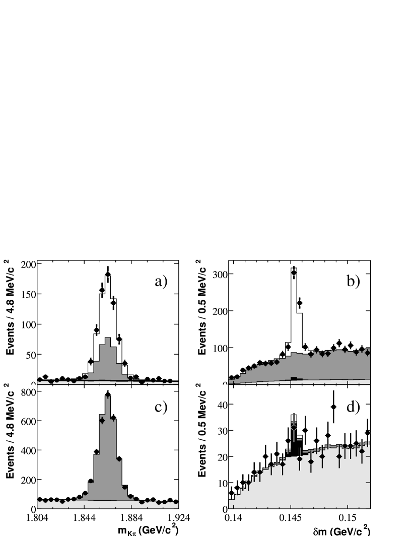
Figure 1: The distribution of the WS data for a) $m_{K\pi}$ with $144.5<\delta m<146.5~{}{\mathrm{\,Me\kern-1.00006ptV\!/}c^{2}}$, b) $\delta m$ with $|m_{K\pi}-m_{D^{0}}|<20~{}{\mathrm{\,Me\kern-1.00006ptV\!/}c^{2}}$, c) $m_{K\pi}$ with $150<\delta m<165~{}{\mathrm{\,Me\kern-1.00006ptV\!/}c^{2}}$, and d) $\delta m$ with $25<|m_{K\pi}-m_{D^{0}}|<60~{}{\mathrm{\,Me\kern-1.00006ptV\!/}c^{2}}$. Data are shown as points with the contributions from the fit overlaid: signal (open), unassociated pion background (dark shaded), double misidentification background (black), and combinatorial background (light shaded).

Table 1: Fit parameter results determined by the full fit, with no constraint on ${x^{\prime}}^{2}$ in the mixing-allowed cases. For the no-mixing cases, $R_{\rm WS}^{(\pm)}=R_{\rm D}^{(\pm)}$. The $+$($-$) signifies $D^{0}$ ($\kern 1.99997pt\overline{\kern-1.99997ptD}{}^{0}$).

Fit case	Parameter	Fit result (${}/10^{-3}$)
		$D^{0}$		$\kern 1.99997pt\overline{\kern-1.99997ptD}{}^{0}$		$D^{0}+\kern 1.99997pt\overline{\kern-1.99997ptD}{}^{0}$
Mixing allowed	$R_{\rm WS}^{(\pm)}$	$\phantom{-0}3.9$		$\phantom{-0}3.2$		$\phantom{-}3.6$
	${x^{\prime(\pm)}}^{2}$	$-0.79$		$-0.17$		$-0.32$
	$y^{\prime(\pm)}$	$\phantom{-}17$		$\phantom{-}12$		$\phantom{-}13$
No mixing	$R_{\rm WS}^{(\pm)}$	$\phantom{-0}3.9$		$\phantom{-0}3.2$		$\phantom{-}3.6$

In Table Search for $D^{0}$-$\kern 1.99997pt\overline{\kern-1.99997ptD}{}^{0}$ Mixing and a Measurement of the Doubly Cabibbo-suppressed Decay Rate in $D^{0}\rightarrow K\pi$ Decays we summarize the central values returned by the fit for the four cases. In Fig. 2 we show the decay-time distribution of the WS sample for the signal and a background region. We select a signal (background) region to provide a sample with 73% signal (50% combinatorial background) candidates based on the reconstructed values of $m_{K\pi}$ and $\delta m$. The selected signal region contains 64% of all signal events according to the fit. In total we observe about 120,000 RS (430 WS) signal decays.

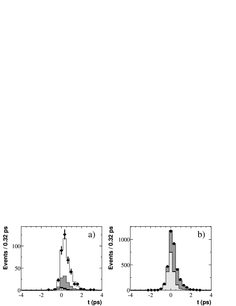
Figure 2: The proper time distribution for the WS candidates in a) the signal region (73% signal purity) and b) a background region (50% combinatorial background). See Fig. 1 for component definitions.

Our fit permits ${x^{\prime}}^{2}$ to take unphysical negative values. The interpretation of non-physical results and error estimates calculated from the log-likelihood surface (LLS) would require a Bayesian analysis where the choice of prior is not clear. In addition, an accurate error estimate from the LLS requires a LLS shape that is not strongly dependent on the outcome of the fit. These requirements are not satisfied here. Therefore, we use a frequentist approach, and construct 95% confidence-level (CL) contours in $({x^{\prime}}^{2}\!\!,y^{\prime})$ utilizing toy MC experiments. In each toy MC experiment we generate a WS dataset (the part sensitive to mixing) for a given $({x^{\prime}}^{2}\!\!,y^{\prime})$ with the same number of $D^{0}$ and $\kern 1.99997pt\overline{\kern-1.99997ptD}{}^{0}$ events as observed in the data, but with a decay-time distribution appropriate for the chosen point. Fit parameters for the $m_{K\pi}$ and $\delta m$ distributions and other parameters not sensitive to mixing are fixed at their fitted values from data. The $\sigma_{t}$ distribution and background fractions from the data fit are used as well. We fit each toy MC dataset, obtaining values for the mixing parameters and the corresponding LLS. We construct contours such that for any point $\vec{\alpha}_{c}=({x^{\prime}}^{2}_{c},y^{\prime}_{c})$ on the contour 95% of the experiments generated at that point will have a log-likelihood difference $\Delta\ln{\cal L}(\vec{\alpha}_{c})=\ln{\cal L}_{\rm max}-\ln{\cal L}(\vec{\alpha}_{c})$ less than the corresponding value $\Delta\ln{\cal L}_{\rm data}(\vec{\alpha}_{c})$ evaluated for the data. ${\cal L}_{\rm max}$ is the maximum likelihood obtained from a fit to either data or a toy MC sample.

Where we assume $C\!P$ conservation we apply this method to the combined $D^{0}$ and $\kern 1.99997pt\overline{\kern-1.99997ptD}{}^{0}$ WS samples. The resulting contour is shown by the dotted line in Fig. 3. The 95% CL limits for $R_{\rm D}$ and for $R_{\rm M}$ are obtained by finding their extreme values on the 95% CL contour.

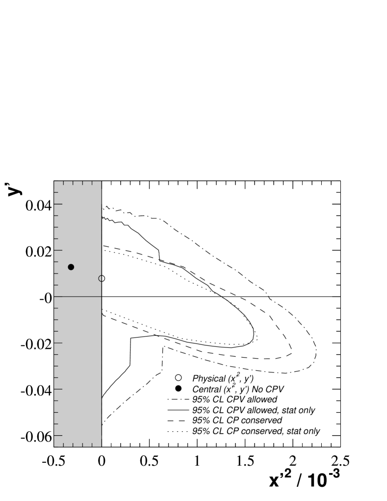
Figure 3: 95% CL limits in $({x^{\prime}}^{2}\!\!,y^{\prime})$ with and without $C\!P$ violation (CPV) allowed. The solid point represents the most likely fit point assuming $C\!P$ conservation and the open circle the same but allowing $C\!P$ violation and forcing ${x^{\prime}}^{2}>0$. The dotted (dashed) line is the statistical (statistical and systematic) contour for the case where no $C\!P$ violation is allowed. The solid and dash-dotted lines are for the corresponding case where $C\!P$ violation is allowed.

To consider $C\!P$ violation, we divide the WS sample into candidates produced as a $D^{0}$ or as a $\kern 1.99997pt\overline{\kern-1.99997ptD}{}^{0}$ and calculate separate contours for $({x^{\prime+}}^{2},y^{\prime+})$ and $({x^{\prime-}}^{2},y^{\prime-})$, each corresponding to a CL of $1-\sqrt{0.05}=77.6\%$. Each point on the $D^{0}$ contour is combined with each point on the $\kern 1.99997pt\overline{\kern-1.99997ptD}{}^{0}$ contour using Eqs. (3)–(5) to produce two potential solutions of {${x^{\prime}}^{2}\!\!$, $y^{\prime}$} for each relative sign of $x^{\prime+}$ and $x^{\prime-}$. The outer envelope of these points is presented as the 95% CL contour in the $({x^{\prime}}^{2}\!\!,y^{\prime})$ plane (see Fig. 3). The peculiar shape of the contour arises from the two potential solutions for each point on the $D^{0}$ and $\kern 1.99997pt\overline{\kern-1.99997ptD}{}^{0}$ contours. This contour is more stringent than the $C\!P$-conserving case in some cases, which is allowed as the definition of coverage is slightly different. No central value for ${x^{\prime}}^{2}$ exists if either ${x^{\prime+}}^{2}$ or ${x^{\prime-}}^{2}<0$.

We summarize results for all four fit cases in Table Search for $D^{0}$-$\kern 1.99997pt\overline{\kern-1.99997ptD}{}^{0}$ Mixing and a Measurement of the Doubly Cabibbo-suppressed Decay Rate in $D^{0}\rightarrow K\pi$ Decays. We obtain limits on the individual mixing parameters by projecting the contours onto the corresponding coordinate axes. Since the no-mixing solution is well within the 95% CL contour, we cannot place limits on $A_{\rm M}$ and $\varphi$.

Table 2: A summary of our results including systematic errors. A central value is reported for the full fit with ${x^{\prime}}^{2}$ fixed at zero. The 95% CL limits are for the case where ${x^{\prime}}^{2}$ was not constrained during the fit.

Fit case	Parameter	Central value	95% CL interval
		(${x^{\prime}}^{2}\!\!=\!0$) (${}/10^{-3}$)	(${}/10^{-3}$)
$C\!P$ violation allowed	$R_{\rm D}$	$3.1$	$2.3$$\;<\;$	$R_{\rm D}<5.2$
	$A_{\rm D}$	$1.2$	$-2.8$$\;<\;$	$A_{\rm D}<4.9$
	${x^{\prime}}^{2}$	$0\phantom{.0}$	${x^{\prime}}^{2}$$\;<\;$	$2.2$
	$y^{\prime}$	$8.0$	$-56$$\;<\;$	$y^{\prime}<39$
	$R_{\rm M}$		$R_{\rm M}$$\;<\;$	$1.6$
No $C\!P$ violation	$R_{\rm D}$	$3.1$	$2.4$$\;<\;$	$R_{\rm D}<4.9$
	${x^{\prime}}^{2}$	$0\phantom{.0}$	${x^{\prime}}^{2}$$\;<\;$	$2.0$
	$y^{\prime}$	$8.0$	$-27$$\;<\;$	$y^{\prime}<22$
	$R_{\rm M}$		$R_{\rm M}$$\;<\;$	$1.3$
No mixing	$R_{\rm D}=(0.357\pm 0.022\hbox{ (stat.)}\pm 0.027\hbox{ (syst.)})\%$
	$A_{\rm D}=0.095\pm 0.061\hbox{ (stat.)}\pm 0.083\hbox{ (syst.)}$
No $C\!P$ viol.	$R_{\rm D}=(0.359\pm 0.020\hbox{ (stat.)}\pm 0.027\hbox{ (syst.)})\%$
or mixing

To estimate systematic uncertainties we evaluate the contributions from uncertainties in the parametrization of the PDFs, detector effects, and event selection criteria. The small systematic effects of fixing the $m_{K\pi}$ and $\delta m$ parameters and the number of events in each category in the final fit is evaluated by varying these parameters within statistical uncertainties while accounting for statistical correlations.

For detector effects such as alignment errors or charge asymmetries we measure their effect on the RS sample. Under the assumption that RS decay is exponential and has no direct $C\!P$ violation, this method is very sensitive. The systematic error due to the size of the MC sample is insignificant since all distributions are obtained from the data.

Each systematic check yields a small shift in the fitted mixing parameters. We use MC experiments to determine the significance of each shift using the same method employed as for the 95% CL statistical contour. We scale the statistical contour with respect to the central fitted point by the factor $\sqrt{1+\sum m_{i}^{2}}$, where $m_{i}$ is the relative significance of each systematic check. For the general case we carry out this procedure for the $D^{0}$ and $\kern 1.99997pt\overline{\kern-1.99997ptD}{}^{0}$ contours separately before combination. In all fits the largest effect for ${x^{\prime}}^{2}$ and $y^{\prime}$ is the $D^{*+}$ momentum selection cut, with $m_{i}^{2}=0.24$; all others are at least three times smaller. For $R_{\rm D}$ the largest effect is the decay-time range. We show contours including systematic errors in Fig. 3 as a dashed line in the $C\!P$ conserving case and as a dash-dotted line in the general case.

In summary, we have set improved limits on $D^{0}$-$\kern 1.99997pt\overline{\kern-1.99997ptD}{}^{0}$ mixing and on $C\!P$ violation in WS decays of neutral $D$ mesons. Our results are compatible with previous measurements Anjos et al. (1988); Aitala et al. (1998); Godang et al. (2000) and with no mixing and no $C\!P$ violation, which agrees with Standard Model predictions.