Neutrino properties studied with a triton source using large TPC detectors

Abstract

Abstract The purpose of the present paper is to study the neutrino properties as they may appear in the low energy neutrinos emitted in triton decay:

$${}^{3}_{1}H\rightarrow^{3}_{2}He+e^{-}+\tilde{\nu}_{e}$$

with maximum neutrino energy of $18.6~{}KeV$. The technical challenges to this end can be summarized as building a very large TPC capable of detecting low energy recoils, down to a few 100 eV, within the required low background constraints. More specifically We propose the development of a spherical gaseous TPC of about 10-m in radius and a 200 Mcurie triton source in the center of curvature. One can list a number of exciting studies, concerning fundamental physics issues, that could be made using a large volume TPC and low energy antineutrinos: 1) The oscillation length involving the small angle $\delta=\sin{2\theta_{13}}$ in the $\nu_{e}$ disappearance experiment is comparable to the length of the detector. Measuring the counting rate of neutrino-electron elastic scattering as function of the distance of the source will give a precise and unambiguous measurement of the oscillation parameters free of systematic errors. In fact first estimations show that a sensitivity of a few percent for the measurement of the above angle. 2) The low energy detection threshold offers a unique sensitivity for the neutrino magnetic moment which is about two orders of magnitude beyond the current experimental limit of $10^{-10}\mu_{B}$. 3) Scattering at such low neutrino energies has never been studied and any departure from the expected behavior may be an indication of new physics beyond the standard model. We present a summary of various theoretical studies and possible measurements.

1 Introduction.

Neutrinos are the only particles in nature, which are characterized by week interactions only. They are thus expected to provide the laboratory for understanding the fundamental laws of nature. Furthermore they are electrically neutral particles characterized by a very small mass. Thus it is an open question whether they are truly neutral, in which case the particle coincides with its own antiparticle , i.e. they are Majorana particles, or they are characterized by some charge, in which case they are of the Dirac type, i.e the particle its different from its antiparticles VERGADOS . It is also expected that the neutrinos produced in week interactions are not eigenstates of the world Hamiltonian, they are not stationary states, in which case one expects them to exhibit oscillations VERGADOS ; VOGBEAC . As a matter of fact such neutrino oscillations seem to have observed in atmospheric neutrino SUPERKAMIOKANDE , interpreted as $\nu_{\mu}\rightarrow\nu_{\tau}$ oscillations, as well as $\nu_{e}$ disappearance in solar neutrinos SOLAROSC . These results have been recently confirmed by the KamLAND experiment KAMLAND , which exhibits evidence for reactor antineutrino disappearance. This has been followed by an avalanche of interesting analyses BAHCALL02 -BARGER02 . The purpose of the present paper is to discuss a new experiment to study the above neutrino properties as they may appear in the low energy neutrinos emitted in triton decay:

$${}^{3}_{1}H\rightarrow^{3}_{2}He+e^{-}+\tilde{\nu}_{e}$$

with maximum neutrino energy of $18.6~{}KeV$. The detection will be accomplished employing gaseous Micromegas,large TPC detectors with good energy resolution and low background GIOMATAR . In addition in this new experiment we hope to observe or set much more stringent constraints on the neutrino magnetic moments. This question has have been very interesting for a number of years and it has been revived recently VogEng -TROFIMOV . The existence of the neutrino magnetic moment can be demonstrated either in neutrino oscillations in the presence of strong magnetic fields or in electron neutrino scattering. The latter is expected to dominate over the weak interaction in the triton experiment since the energy of the outgoing electron is very small. Furthermore the possibility of directional experiments will provide additional interesting signatures. Even experiments involving polarized electron targets are beginning to be contemplated RASHBA . There are a number of exciting studies, of fundamental physics issues, that could be made using a large volume TPC and low energy antineutrinos:

• The oscillation length is comparable to the length of the detector. Measuring the counting rate of neutrino elastic scattering as function of the distance of the source will give a precise and unambiguous measurement of the oscillation parameters free of systematic errors. First estimations show that a sensitivity of a few percent for the measurement of $\sin^{2}{\theta_{13}}$.

• The low energy detection threshold offers a unique sensitivity for the neutrino magnetic moment, which is about two orders of magnitude beyond the current experimental limit of $10^{-10}\mu_{B}$. In our estimates below we will use the optimistic value of $10^{-12}\mu_{B}$.

• Scattering at such low neutrino energies has never been studied before. In addition one may exploit the extra signature provided by the photon in radiative electron neutrino scattering. As a result any departure from the expected behavior may be an indication of physics beyond the standard model.

In the following we will present a summary of various theoretical studies and possible novel measurements

2 The neutrino mixing.

We suppose that the neutrinos produced in week interactions are not stationary states, i.e. they are not eigenstates of the Hamiltonian. In this case the week eigenstates are linear combinations of the mass eigenstates VERGADOS :

$$\nu^{0}_{eL}=\sum^{3}_{k=1}~{}U^{(11)}_{ek}~{}\nu_{kL}+\sum^{3}_{k=1}~{}U^{(12)}_{ek}~{}N_{kL},$$ (1)

$$\nu^{0}_{eR}=\sum^{3}_{k=1}~{}U^{(21)}_{ek}~{}\nu_{kL}+\sum^{3}_{k=1}~{}U^{(22)}_{ek}~{}N_{kL},$$ (2)

the fields

$$\nu_{k}~{}(N_{k})$$

are the light (heavy) Majorana neutrino eigenfields with masses
$m_{k}~{}$ ($m_{k}<<1$ MeV) and $M_{k}$ ($M_{k}>>1$ GeV).

The matrices

$$U^{(11)}_{ek}~{}~{},~{}~{}U^{(22)}_{ek}$$

are approximately unitary, while the matrices

$$U^{(12)}_{ek}~{}~{},~{}~{}U^{(21)}_{ek}$$

are very small (of order of mass of the up quark divided by that of the heavy neutrino, $m_{N}\approx 10^{12}~{}GeV$)
$\nu_{k},N_{k}$ satisfy the Majorana condition:

$$\nu_{k}\xi_{k}=C~{}{\overline{\nu}}_{k}^{T}~{},~{}N_{k}\Xi_{k}=C~{}{\overline{N}}_{k}^{T}$$

where C denotes the charge conjugation. The quantities:

$$\xi_{k}=e^{i\lambda_{k}}~{},~{}\Xi_{k}=e^{i\Lambda_{k}}$$

are phase factors, which guarantee that the eigenmasses are positive. They are relevant even in a CP conserving theory since even then some of the phases $\lambda_{k}~{},~{}\Lambda_{k}$ can take the value $\pi$.

In what follows we will ignore the heavy neutrino components, i.e. we will assume that $U=U^{11}$.

3 Neutrino masses as extracted from various experiments

At this point it instructive to elaborate a little bit on the neutrino mass combinations entering various experiments.

• Neutrino oscillations.
  These in principle, determine the mixing matrix and two independent mass-squared differences, e.g.

  $$\Delta m^{2}_{21}=m^{2}_{2}-m^{2}_{1}~{}~{},~{}~{}\Delta m^{2}_{31}=m^{2}_{3}-m^{2}_{1}$$

  They cannot determine:

  1. the scale of the masses, e.g. the lowest eigenvalue $m_{1}$ and

  2. the two relative Majorana phases.

• The end point triton decay.

  This can determine one of the masses, e.g. $m_{1}$ by measuring:

  $$(m_{\nu})_{1\beta}\equiv m_{\nu}=|\sum_{j=1}^{3}U^{*}_{ej}U_{ej}m^{2}_{j}|^{1/2}\,,~{}U=U^{11}$$ (3)

  Once $m_{1}$ is known one can find
  

  $$m_{2}=[\delta m^{2}_{21}+m^{2}_{1}]^{1/2}~{}~{},~{}~{}m_{3}=[\delta m^{2}_{31}+m^{2}_{1}]^{1/2}$$

  provided, of course that the mixing matrix is known.
  Since the Majorana phases do not appear, this experiment cannot differentiate between Dirac and Majorana neutrinos. This can only be done via lepton violating processes, like:

• $0\nu\beta\beta$ decay.

  This provides an additional independent linear combinations of the masses and the Majorana phases.

  $$\langle m_{\nu}\rangle_{2\beta}\equiv\langle m_{\nu}\rangle=|\sum_{j=1}^{3}U_{ej}U_{ej}e^{i\lambda_{j}}m_{j}|$$ (4)

• and muon to positron conversion.

  This also provides an additional relation

  $$\langle m_{\nu}\rangle_{\mu e+}=|\sum_{j=1}^{3}U^{*}_{\mu j}U^{*}_{ej}e^{-i\lambda_{j}}m_{j}|\,.$$ (5)

Thus the two independent relative CP phases can in principle be measurable. So these three types of experiments together can specify all parameters not settled by the neutrino oscillation experiments.

Anyway from the neutrino oscillation data alone we cannot infer the mass scale. Thus the following scenarios emerge

1. the lightest neutrino is $m_{1}$ and its mass is very small. This is the normal hierarchy scenario. Then:

   $$\Delta m^{2}_{21}=m^{2}_{2}~{}~{},~{}~{}\Delta m^{2}_{31}=m^{2}_{3}$$

2. The inverted hierarchy scenario. In this case the mass $m_{3}$ is very small. Then:

   $$\Delta m^{2}_{21}=m^{2}_{2}-m^{2}_{1}~{}~{},~{}~{}\Delta m^{2}_{31}=m^{2}_{1}$$

3. The degenerate scenario. In such a situation all masses are about equal and much larger than the differences appearing in neutrino oscillations. In this case we can obtain limits on the mass scale as follows:

   • From triton decay. Then LOBASHEV

     $$m_{1}\approx(m_{\nu})_{1\beta}\leq 2.2eV$$

     This limit is expected to substantially improve in the future KATRIN .

   • From $0\nu~{}\beta\beta$ decay. The analysis now depends on the mixing matrix and the CP phases of the Majorana neutrino eigenstates VERGADOS (see discussion below). If the relative phase of the CP eigenvalues of the two strongly admixed states is zero, the best limit coming from $0\nu~{}\beta\beta$ decay is:

     $$m_{1}\approx\langle m_{\nu}\rangle_{2\beta}\leq 0.5~{}eV$$

     On the other hand it is

     $$m_{1}\approx\frac{\langle m_{\nu}\rangle_{2\beta}}{\cos{2\theta_{solar}}}\approx 2\langle m_{\nu}\rangle_{2\beta}\leq 1.0~{}eV,$$

     if this relative phase is $\pi$.

     These limits are going to greatly improve in the next generation of experiments, see e.g. the review by Vergados VERGADOS and the experimental references therein.

4 Experimental considerations

In this section we will focus on the experimental considerations

4.1 The radial TPC concept

One of the attractive features of the gaseous TPC is its ability to precisely reconstruct particle trajectories without precedent in the redundancy of experimental points, i.e. a bubble chamber quality with higher accuracy and real time recording of the events. Many proposals are actually under investigation to exploit the TPC advantages for various astroparticle projects and especially solar or reactor neutrino detection and dark matter search GORO -SNOWDEN . A common goal is to fully reconstruct the direction of the recoil particle trajectory, which together with energy determination provide a valuable piece of information. The virtue of using the TPC concept in such investigations has been now widely recognized and a special International Workshop has been recently organized in Paris PARIS . The study of low energy elastic neutrino-electron scattering using a strong tritium source was envisaged in by Bouchez and Giomataris BG employing a large volume gaseous cylindrical TPC. We will present here an alternate detector concept with different experimental strategy based on a spherical TPC design. A sketch of the principal features of the proposed TPC is shown in Fig. 1.

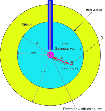
Figure 1: The principal features of the proposed TPC.

It consists of a spherical vessel of 10 meters in radius that contains about 20 Tons of gas made by a thin low radioactivity acrylic metalized in the inner surface to provide electric contact to the high voltage (drift voltage of about -100 kV). It is located in a cavern of an underground laboratory and separated from the rock by 1 meter shield (2-3 meters water equivalent of high purity shielding). The ground plane is another smaller sphere about 50 cm in radius which carries the detector plane and defines with the drift volume a gas target volume 9.5 m long; ionization electrons released during the elastic scattering with the target gas are drifting to the detector where are collected and amplified. There are actually many gaseous detectors adequate for this experiment but we will focus our detection strategy on Micromegas GIOMATAR , a new technology, which is now widely recognized and used by many particle physics experiments. The 200 Mcurie tritium source container is a sphere 20-cm in radius. Neutrino emitted can produce electron recoil in the gaseous volume by the elastic scattering reaction and the distance from the center of curvature is detected. The concept of the spherical TPC simplifies the whole structure since:

• It provides in a simple way a good estimation of the radial location (depth) of the neutrino-electron elastic scattering

• It does not require a special field cage as in the conventional-cylindrical TPC.

• the converging radial electric field is strongly focussing the drifting electron charges providing a reasonable size of the detection plane (about $4m^{2}$)

• Last, but not least, the whole structure is relatively simple and cheap with a very-reasonable number of detectors and electronics

A schematic view of the inner part vessel with the detector and the tritium source is shown in Fig. 2.

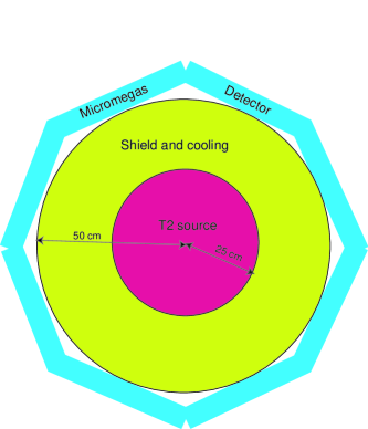
Figure 2: A schematic view of the inner part of the vessel with the detector and the tritium source.

Our approach is radically different from all other neutrino oscillation experiments in that it measures the neutrino interactions, as a function of the distance source-interaction point, with an oscillation length that is fully contained in the detector; it is equivalent to many experiments made in the conventional way where the neutrino flux is measured in a single space point. Furthermore, since the oscillation length is comparable to the detector depth, we expect an exceptional signature: a counting rate oscillating from the triton source location to the depth of the gas volume, i.e. at first a decrease, then a minimum and finally an increase. In other words we will have a full observation of the oscillation process as it has already been done in accelerator experiments with neutral strange particles ($K^{0}$).

4.2 The gas vessel

The external drift-electrode sphere will be made using low background materials. Polypropylene or polyethylene have the advantage that they do not contain oxygen in the bulk material. The drift sphere could be enclosed in an external pressure vessel containing, for instance, a low-radioactivity appropriate solid or liquid that is used as a buffer shield to cope with the rock background emission. Indeed the various background contributions evaluated by other groups show that natural radioactivity of the rock turns out to be by far the most important background component in such investigations. The gas volume acts both as target and detector of neutrino-electron elastic scattering events. The total elastic scattering cross section for the triton neutrinos is $0.58\times 10^{-47}cm^{2}$ integrating between 100eV and 1.27 keV, the maximum electron recoil energy. Filling the gas volume with Xenon gas at atmospheric pressure ( containing about $6\times 10^{30}$ electrons) will allow observation of 3500 elastic interactions/year using a 200 MCurie, 20 kg tritium source. The versatility of the gas volume Micromegas detector scheme allows a variety of gaseous targets: Xenon can be used at atmospheric pressure and has not any intrinsic radioactivity. It contains, however, a large fraction of 85Kr that is a beta emitter with end point energy of 700 keV and a quite short time of life of 10.7 years. However only a small part of the spectrum, about $0.1\%$, is contained in our energy bandwidth. First estimates show that a removal of Krypton at the level of $10^{-12}$ is required. The later requirement is about 3 orders of magnitude lower than in the liquid Xenon future WIMP searches projects ICHIGE ; LUSCHER . Since, however, Xenon is the most expensive noble gas other gas targets should be considered. Argon is very-cheap material and must operate at a pressure of about 2.5 bars. It has some intrinsic radioactivity mainly due to a beta emitting isotope ${}^{42}Ar$ ($t_{1/2}=33~{}y$, $E_{max}=565~{}keV$). The Icarus group ICARUS has measured the ratio ${}^{42}Ar/^{38}Ar$ to be less than $7\times 10^{-22}$; our first preliminary estimations show that the effect of this radioactivity is quite small and thus Argon should not be excluded as target for this experiment. Neon has no intrinsic radioactivity and because of its low boiling point is easy to purify and clean for unwanted impurities, but it must be used at a pressure of 5 bars. Helium is low cost and the cleanest gaseous target, but it has the drawback that its density is quite low , $166gr/m^{3}$ at NTP, which implies that it should operate at a pressure of about 25 bars.

The TPC is located underground and it is fully enclosed by the drift spherical electrode, which at the same time constitutes an efficient Faraday cage. We can then reasonably assume that the noise seen by the TPC will be generated only by its internal components. The radio purity of the various elements is one of the main challenges and, to deal with it, we need other groups participating in this project, in particular those who are world leaders in ultraslow background technology as well.

4.3 The detector

The energy released by ionizing particles (low energy electron recoils) in the drift volume will produce local charge clouds to be transported to the detector plane in order to be amplified and collected on the anodes. Since we are dealing with low energy recoils we need a high gain detector with good time resolution and capable to reject other backgrounds induced by Compton scattering of gamma rays, beta decays or other ionizing particles, such as small contaminants of radon, present in underground facilities. To meet the various objectives we will concentrate on Micromegas technology. The European experiment to search for solar axions ZIOUTAS ; AALSETH , CAST, is using the Micromegas idea, and several successful experiments have also been using such charge readout MAGNON ; ADRIAN . MICROMEGAS (MICROMEsh GAseous Structure) GIOMA98 ; DERRE99 ; DERRE01 is a gaseous two - stage parallel-plate avalanche chamber design consisting of a narrow $50-100\mu m$ amplification gap and a thick conversion region, separated by a light conducting micromesh, usually made of electroformed nickel or copper. Electrons released in the gas-filled conversion gap by an ionizing particle are transported to the amplification gap where they are multiplied in an avalanche process. In most of the applications signals induced on anode elements (strips or pads) are providing a precise x-y spatial projection of the energy deposition that is a key element for efficient background rejection. For this project such precise two- dimensional determination is not required and will be only optional in the cases for which the background level is so high that additional rejection will be needed. The detector element has a hexagonal-flat shape with a dimension of about 20- cm. A lot of such detector elements, about $100$, are arranged around a spherical surface. Each detector has a single read-out that consists of a low noise charge preamplifier (about 50 ns peaking time) followed by fast shaper and a 100 MHz flash ADC. Building such Micromegas detectors do not present a major technological effort since that size counters are routinely used in particle beams; larger detectors of $40\times 40cm^{2}$ are nicely operating in COMPASS experiment. Detecting such low energy recoils with Micromegas detectors at NTP is not a big deal. At high pressure there is a certain drop of the gain which is proportional to the value of the pressure. In the later case we could rely on various future developments and, in this context, we should point out the progress made in the framework of the HELLAZ GORO experiment. An exhaustive study, made for solar neutrino detection, using high pressure helium has shown the ability of the Micromegas detector to reach high gains (about $10^{6}$) at $20$  bars, which opens the possibility to lower the detection threshold to a single electron and therefore the single electron counting.

To summarize:

• The aim of the proposed detector will be the detection of very low energy neutrinos emitted by a strong tritium source through their elastic scattering on electrons of the target.

• The $(\nu,e)$ elastic differential cross section is the sum of the charged and neutral current contributions (see sec. 7) and is a function of the energy. It is, however, it is quite small, see Eq. (20).

• Integrating this cross section up to energies of $15~{}KeV$ we get a very small value, $\sigma=0.4\times 10^{-47}cm^{2}$. This means that, to get a significant signal in the detector, for 200 Mcurie tritium source (see next section) we will need about 20 kilotons of gaseous material.

• The elastic $(\nu,e)$ cross section, being dominated by the charged current, especially for low energy electrons (see Fig. 10 below), will be different from that of the other flavors, which is due to the neutral current alone. This will allow us to observe neutrino oscillation enabling a modulation on the counting rate along the oscillation length. The effect depends on the electron energy T as is shown in sec. 6

4.4 The neutrino source

Tritium is widely produced in nuclear reactors using light water and especially in those using heavy water, the back-up production technology being the Linear accelerator where tritium is usually made by capturing neutrons in ${}^{3}_{2}He$ (helium gas). Tritium has a relatively short half-life of 12.3 years, which is long enough to ensure a high neutrino flux for several years of experimental investigations. It emits a low energy beta particle (energy of about 5 keV), and an anti-neutrino (energy of about 5 keV ) and in the process decays to Helium-3 which is not radioactive. Absorbing such low energy beta particles is not a big deal, a few millimeter copper sheet will stop the total emitted beta energy or soft X-rays from bremsstrahlung process. The total power produced is 4 kwatt/20 kg that must be dissipated by an appropriate cooling system; a liquid circulating system in the volume surrounding the source must be designed. Temperature measurement of the heating loss will provide the neutrino flux to within one percent. Large amount of tritium radioactive material ($>>20~{}kgr$) are stored in various parts of the world due to the reduction of nuclear weapons or production by nuclear reactors (in particular those using heavy water).

The container of the source should be carefully designed in order to fulfill the safety requirements and, at the same time, provide a flexible moving system for source on- off measurements. It could be made, for instance, of low radioactivity copper about 1 cm thick. The space between the source and the detector plane is filled by a high radioactive purity material which must ensure, at the same time, adequate cooling to compensate for the power produced by the triton emission energy. The design, construction, test and transport of the source system to the underground laboratory is certainly a delicate project that requires a team of specialized physicists and engineers. We would like also to mention a more exhaustive study of such intense tritium source made by another group NEGANOV .

4.5 Simulation and results

We assume a spherical type detector, described in the previous section, filed with Xenon gas at NTP and a tritium source of 20 kg, providing a very-high intensity neutrino emission of $6\times 10^{18}/s$. The Monte Carlo program is simulating all the relevant processes:

• Beta decay and neutrino energy random generation

• Oscillation process of $\nu_{e}$ due to the small mixing $\theta_{13}$ (see Eq. 6 below).

• Neutrino elastic scattering with electrons of the gas target

• Energy deposition, ionization processes and transport of charges to the Micromegas detector.

The collected charge on the detector will provide the electron recoil energy with a good precision. The lack of trigger signal, however, will not allow a direct measurement of the radial distance in the conventional way used in drift chambers. We have adopted a novel method of estimating the radial dimension, which relies on the excellent time resolution of the detector (below 1 ns has been achieved GIOMA98 ) and its ability to detect low amount of charges (down to single electrons). The idea is to exploit the large longitudinal diffusion of charges, produced by energy deposition of the recoil electron, during their long drift to the detector plane. The special electric configuration with a very weak value ($E=10~{}Volt/cm$) at the highest distance (at 10 m) works towards this goal; the longitudinal diffusion at such low field is roughly proportional to E and the drift velocity inversely proportional to E, enhancing time dispersion of the collected signals. Measuring the arrival time of the ionization electrons and therefore their time dispersion will provide a rough but good estimation of the radial drift distance (L).

First Monte Carlo simulate are giving a resolution of better than 10 cm, which is good enough for our need. In Fig. 3 the energy distribution of the detected neutrinos, assuming a detection threshold of 200 eV, is exhibited. The energy is concentrated around 13 keV with a small tail to lower values.

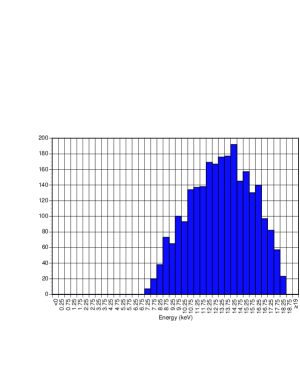
Figure 3: Neutrino energy distribution with an energy cutoff of $200~{}eV$.

In Figs 6 and 7 below we show the number of detected elastic events as function of the distance L in bins of one meter for several hypothesis for the value of the mixing angle $\theta^{2}_{13}=0.170,0.085$ and $0.045$. We observe a decreasing of the signal up to about 6.5 m and then a rise. Backgrounds are not yet included in this simulation but the result looks quite promising; even in the case of the lowest mixing angle the oscillation is seen, despite statistical fluctuations. We should point out that in the context of this experiment complete elimination of the backgrounds is not necessary. It is worth noting that:

• A source-off measurement at the beginning of the experiment will yield the background level to be subtracted from the signal.

• Fitting the observed oscillation pattern will provide, for the first time, a stand alone measurement of the oscillation parameters, the mixing angle and the square mass square difference.

• Systematic effects due to backgrounds or to bad estimates of the neutrino flux, which is the main worry in most of the neutrino experiments, are highly reduced in this experiment.

5 A simple phenomenological neutrino mixing matrix

The available neutrino oscillation data (solar SOLAROSC and atmospheric SUPERKAMIOKANDE )as well as the KamLand KAMLAND results can adequately be described by the following matrix:

$\left(\begin{array}[]{c}\nu_{e}\\ \nu_{\mu}\\ \nu_{\tau}\end{array}\right)=\left(\begin{array}[]{ccc}c&s&\delta\\ -\frac{s+c\delta}{\sqrt{2}}&\frac{c-s\delta}{\sqrt{2}}&\frac{1}{\sqrt{2}}\\ \frac{s-c\delta}{\sqrt{2}}&-\frac{c+s\delta}{\sqrt{2}}&\frac{1}{\sqrt{2}}\\ \end{array}\right)=\left(\begin{array}[]{c}\nu_{1}\\ \nu_{2}\\ \nu_{3}\end{array}\right)$

Up to order $\delta^{2}$ ($\delta^{2}=4\times 10^{-2}$). Sometimes we will use $\theta_{13}$ instead of $\delta$. In the above expressions

$$c=\cos\theta_{solar}~{},~{}s=\sin\theta_{solar}$$

This angle is determined from the solar neutrino data SOLAROSC , BAHCALL02 -BARGER02

$$\tan^{2}\theta_{solar}\approx 0.35-0.42$$

while the analysis of KamLAND results BAHCALL02 -BARGER02 yields:

$$\tan^{2}\theta_{solar}\approx 0.64-0.79$$

6 Simple expressions for neutrino oscillations

• Solar neutrino Oscillation (LMA solution) is given by:

  $$P(\nu_{e}\rightarrow\nu_{e})\approx 1-(\sin 2\theta_{solar})^{2}\sin^{2}(\pi\frac{L}{L_{21}})$$

  $$L_{21}=\frac{4\pi E_{\nu}}{\Delta m^{2}_{21}}$$

  The analysis of both the neutrino oscillation experiments as well as KamLAND BAHCALL02 -BARGER02 yield

  $$\Delta m^{2}_{21}=|m_{2}^{2}-m_{1}^{2}|=(5.0-7.5)\times 10^{-5}(eV)^{2}$$

• The Atmospheric Neutrino Oscillation takes the form:

  $$P(\nu_{\mu}\rightarrow\nu_{\tau})\approx 2(\cos\theta_{solar})^{2}\sin^{2}(\pi\frac{L}{L_{32}})$$

  $$L_{32}=\frac{4\pi E_{\nu}}{\Delta m^{2}_{32}}\rightarrow\Delta m^{2}_{32}=|m_{3}^{2}-m_{2}^{2}|=2.5\times 10^{-3}(eV)^{2}$$

• We conventionally write

  $$\Delta m^{2}_{32}=\Delta m_{atm}^{2}~{}~{},~{}~{}\Delta m^{2}_{21}=\Delta m_{sol}^{2}$$

• Corrections to disappearance experiments

  $$P(\nu_{e}\rightarrow\nu_{e})=1-\frac{(\sin 2\theta_{solar})^{2}\sin^{2}(\pi\frac{L}{L_{21}})+4\delta^{2}\sin^{2}(\pi\frac{L}{L_{32}})}{(1+\delta^{2})^{2}}$$ (6)

• The probability for $\nu_{e}\rightarrow\nu_{\mu}$ oscillation takes the form:

  $$P(\nu_{e}\rightarrow\nu_{\mu})=\frac{\left[(\sin 2\theta_{solar})^{2}+\delta\sin{4\theta_{solar}}\right]\sin^{2}(\pi\frac{L}{L_{21}})+4\delta^{2}\sin^{2}(\pi\frac{L}{L_{32}})}{(1+\delta^{2})^{2}}$$ (7)

• While the oscillation probability $\nu_{e}\rightarrow\nu_{\tau}$ becomes:

  $$P(\nu_{e}\rightarrow\nu_{\tau})=\frac{\left[(\sin 2\theta_{solar})^{2}-\delta\sin{4\theta_{solar}}\right]\sin^{2}(\pi\frac{L}{L_{21}})+4\delta^{2}\sin^{2}(\pi\frac{L}{L_{32}})}{(1+\delta^{2})^{2}}$$ (8)

From the above expression we see that the small amplitude $\delta$ term dominates in the case of triton neutrinos ($L\leq L_{32}~{},L_{21}=50L_{32}$)

In the proposed experiment the neutrinos will be detected via the recoiling electrons. If the neutrino-electron cross section were the same for all neutrino species one would not observe any oscillation at all. We know, however, that the electron neutrinos behave very differently due to the charged current contribution, which is not present in the other neutrino flavors. Thus the number of the observed electron events ($ELEV$) will vary as a function of $L/E_{\nu}$ as follows:

$$ELEV\propto\left[1-\chi(E_{\nu},T)\frac{(\sin 2\theta_{solar})^{2}\sin^{2}(\pi\frac{L}{L_{21}})+4\delta^{2}\sin^{2}(\pi\frac{L}{L_{32}})}{(1+\delta^{2})^{2}}\right]\frac{d(\sigma(\nu_{e},e^{-}))}{dT}$$ (9)

where

$$\chi(E_{\nu},T)=\frac{(d\sigma(\nu_{e},e^{-}))/dT-d(\sigma(\nu_{\alpha},e^{-}))/dT}{d(\sigma(\nu_{e},e^{-}))/dT}$$

($\nu_{\alpha}$ is either $\nu_{\mu}$ or $\nu_{\tau}$). In other words $\chi$ represents the fraction of the $\nu_{e}$-electron cross-section, $\sigma(\nu_{e},e^{-})$, which is not due to the neutral current. Thus the apparent disappearance oscillation probability will be quenched by this fraction. As we will see below, see section 7, the parameter $\chi$, for $sin^{2}\theta_{W}=0.2319$, can be cast in the form:

$$\chi(E_{\nu},T)=2\frac{2-(m_{e}T/E^{2}_{\nu})}{4.6199+0.4638(1-T/E{\nu})^{2}-1.4638(m_{e}T/E^{2}_{\nu})}$$ (10)

We thus see that the parameter $\chi$ depends not only on the neutrino energy, but on the electron energy as well, see Figs 4-5.

Figure 4: The parameter $\chi$ as a function of the electron kinetic energy T for $E_{\nu}=9.0~{}KeV$ on the left and $12.0~{}KeV$ on the right.

Figure 5: The parameter $\chi$ as a function of the electron kinetic energy T for $E_{\nu}=15.0~{}KeV$ on the left and $18.0~{}KeV$ on the right.

It interesting to see that, for a given neutrino energy, $\chi$, as a function of $T$, is almost a straight line. We notice that, for large values of $T$, the factor $\chi$ is suppressed, which is another way of saying that, in this regime, in the case of $(\nu_{e},e^{-})$ differential cross-section the charged current contribution is cancelled by that of the neutral current. In order to simplify the analysis one may try to replace $\chi$ by an average value $\bar{\chi}(E_{\nu})$, e.g. defined by:

$$\bar{\chi}(E_{\nu})=\frac{1}{T_{max}(E_{\nu})}\int_{0}^{T_{max}(E_{\nu})}\chi(E_{\nu},T)~{}dT$$ (11)

Then surprisingly one finds $\bar{\chi}(E_{\nu})$ is independent of $E_{\nu}$ with a constant value of $0.42$. This is perhaps a rather high price one may have to pay for detecting the neutrino oscillations as proposed in this work.

6.1 Modification of neutrino oscillation in a magnetic field due to the magnetic moment

In the presence of a neutrino magnetic moment (see the Appendix for derivations) one finds that the electron neutrino disappearance probability in the three generation model discussed above with Majorana neutrinos takes the form:

$$P(\nu_{e}L\rightarrow\nu_{e}L)\approx 1 - \frac{\left[\sin^{2}{2\theta_{1}}^{2}+sin^{2}{2\theta}\cos^{2}{2\theta_{1}}\right]\sin^{2}{\pi\frac{L}{L_{21}}}\sqrt{1+(\xi\frac{B}{1T})^{2}}}{(1+\delta^{2})^{2}}$$ (12)

$$- \frac{4\delta^{2}\sin^{2}(\pi\frac{L}{L_{32}})}{(1+\delta^{2})^{2}}$$ (13)

The parameter $\theta_{1}$ describes the $L-R$ mixing due to the neutrino magnetic moment (see the Appendix).

In the case of Dirac neutrinos (see the Appendix) the above equation becomes

$$P(\nu_{e}L\rightarrow\nu_{e}L)\approx 1-\frac{(\sin 2\theta)^{2}\sin^{2}{\pi\frac{L}{L_{21}}}\cos^{2}{(\mu_{\nu}BL)}-\sin^{2}{(\mu_{\nu}BL})+4\delta^{2}\sin^{2}{\pi\frac{L}{L_{32}}}}{(1+\delta^{2})^{2}}$$ (14)

The parameter $\xi$ describes the mixing due to the neutrino magnetic moment (see the Appendix) and has been evaluated in a magnetic field of strength $1T$, is given as follows:

$$\xi=\frac{4\mu_{\nu}E_{\nu}~{}1T}{\delta m^{2}_{21}}$$

For $L_{12}>>L$, $L_{23}\approx L$ and for small magnetic moment the above equations become:

$$P\left(\nu_{eL}\rightarrow\nu_{eL}\right)\approx 1-\frac{\left[\sin{2\theta}^{2}+\xi^{2}(B/1T)^{2}\right](\pi\frac{L}{L_{21}})^{2}+4\delta^{2}\sin^{2}{\pi\frac{L}{L_{32}}}}{(1+\delta^{2})^{2}}$$ (15)

We see that in the experiment involving a triton target one will actually observe a sinusoidal oscillation as a function of the source-detector distance $L$ with an amplitude, which is proportional to the square of the small mixing angle $\delta$. The relevant oscillation length is given by:

$$L_{32}=2.476m\frac{E_{\nu}(MeV)}{\Delta m^{2}_{32}((eV)^{2})}$$

In the present experiment for an average neutrino energy $E_{\nu}\approx 13KeV$ and $\Delta m^{2}_{32}=2.5\times 10^{-3}(eV)^{2}$ we find

$$L_{32}\approx 13.5m$$

In other words the maximum will occur close to the source at about $L=7.5m$. Simulations of the above neutrino oscillation involving $\nu_{e}$ disappearance due to the large $\Delta m^{2}=2.5\times 10^{-3}$, i.e associated with the small mixing $\delta$, are shown in Figs 6- 7. One clearly sees that the expected oscillation, present even for $\delta$ as low as $0.045$, will occur well inside the detector.

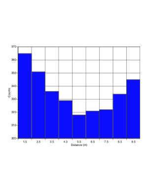
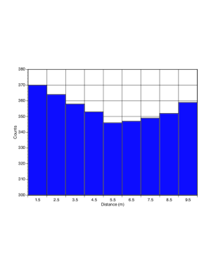
Figure 6: Simulation of $\nu_{e}$ disappearance due to the large $\Delta m^{2}=2.5\times 10^{-3}(eV)^{2}$ involving the small mixing angle $\delta$. On the left we show results for $\delta=0.170$, while on the right we show results for $\delta=0.085$. One expects to unambiguously see the full oscillation inside the detector with the maximum disappearance occurring around $5.5m$. This a bit smaller than the calculated value of $7.5m$ due to the fact that the simulation takes into account all energies.

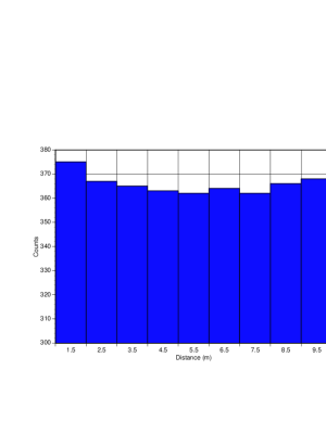
Figure 7: The same as in Fig. 6 for $\delta=0.045$.

Superimposed on this oscillation one will see an effect due to the smaller mass difference, which will increase quadratically with the distance $L$. In the presence of a magnetic field this amplitude will also depend quadratically in the magnetic field. The product of the mixing angle with the mass-squared difference in one hand and the effect of the magnetic moment squared on the other are additive. This is indeed very beautiful experimental signature. Its practical exploitation depends, of course, on the actual value of the parameter $\xi$. This can be cast in the form:

$$\xi=2\times 10^{-10}\frac{\mu_{\nu}}{10^{-12}\mu_{B}}\frac{E_{\nu}}{0.5MeV}\frac{10^{-2}~{}eV^{2}}{\delta m^{2}_{21}}$$ (16)

It is unfortunately clear that the parameter $\xi$ is unobservable in all experiments involving low energy neutrinos, if the magnetic moment is of the order of $10^{-12}\mu_{B}$. This is particularly true for the triton decay experiments with maximum energy of 18.6 KeV.

6.2 Modification of neutrino oscillations due to neutrino decay

The effect of the finite life time of neutrinos on the oscillation pattern VogEng has mainly been investigated in connection with solar neutrinos, see, e.g., Indumathi INDUMATHI and references therein. If in fact the decay widths are very small only in the case of very long distances one may have a detectable effect. In spite of this we will examine what effects, if any, the finite neutrino life time may have on our experiment or other non-solar experiments. For the readers convenience some useful formulas are given in the appendix. We find that the decay width for the transition $i\rightarrow j$ is given by the formula PAKVASA :

$$\Gamma_{i}=K_{0}\frac{m_{i}^{2}-m_{j}^{2}}{E_{\nu}}(1+\frac{m_{j}}{m_{i}})^{2}$$ (17)

For more complete expressions, involving Majoron models VERGADOS ; MAJORON , the reader is referred to the literature BEACOM ; RATES . We prefer to use here the dimensionless quantity $K_{0}$ rather the decay constant $\alpha=m_{i}/\tau_{0i}$. These quantities are related via the equation $K_{0}=\alpha/\Delta m^{2}$. A limit on the decay constant $\alpha$ exists from the SNO data BEACOM , $\alpha\leq 10^{4}(m/s)=7\times 10^{-12}(eV)^{2}$, but it is not very firm since depends on certain assumptions. Anyway this leads to $K_{0}\leq 2.6\times 10^{-9}$. For the proposed experiment, $L\approx 10m$ $<E_{\nu}>=10KeV$, if we demand $\Gamma L/2\approx 3$, the dimensionless quantity $K_{0}$ has to be of order unity. For $K_{0}=0.5$ in the hierarchical case, $m_{i}^{2}\approx\Delta m^{2}=m_{i}^{2}-m_{j}^{2}$, we obtain:

$$\Gamma_{3}=1.0\times 10^{-7}eV~{}~{}~{},~{}~{}~{}\Gamma_{2}=3.0\times 10^{-9}eV$$

These are much larger than those obtained from the above bound and $\Gamma\approx 10^{-26}eV\Leftrightarrow\tau=10^{11}s$ or typical values expected in reasonable theoretical models VERGADOS . In the case of solar neutrinos a value of $K_{0}\approx 10^{-9}$ may be adequate, see Indumathi INDUMATHI .

From the formulas in the appendix (Eqs. (46 )- (49)) we see that at sufficiently long distances the neutrino oscillation is wiped out by the finite neutrino lifetime. It is amusing to remark that for the rather unrealistic case $\Gamma_{3}L/2\approx 0.1$ the oscillation proportional to $\delta^{2}$, the observation of which is one of the main goals of this experiment, will be suppressed to $10\%$ of its value without the presence of neutrino decay. In other words in this case the extraction of the parameter $\delta$ may not be straightforward.

7 Elastic electron neutrino scattering.

The elastic neutrino electron scattering is very crucial in our investigation, since it will be employed for the detection of neutrinos.

We have seen in the previous section that the detection of the neutrino magnetic moment in laboratory neutrino oscillation experiments is extremely difficult, if not impossible. The elastic electron neutrino scattering offers a better possibility. Following the work of Vogel and Engel VogEng one can write the relevant differential cross section as follows:

$$\frac{d\sigma}{dT}=\left(\frac{d\sigma}{dT}\right)_{week}+\left(\frac{d\sigma}{dT}\right)_{EM}$$ (18)

We ignored the contribution due to the neutrino charged radius.

The cross section due to weak interaction alone takes the form VogEng :

$$\left(\frac{d\sigma}{dT}\right)_{week}=\frac{G^{2}_{F}m_{e}}{2\pi}\left[(g_{V}+g_{A})^{2}+(g_{V}-g_{A})^{2}[1-\frac{T}{E_{\nu}}]^{2}+(g_{A}^{2}-g_{V}^{2})\frac{m_{e}T}{E^{2}_{\nu}}\right]$$ (19)

where

$$g_{V}=2\sin^{2}\theta_{W}+1/2~{}~{}for~{}~{}\nu_{e}~{}~{}~{}~{},~{}~{}~{}~{}g_{V}=2\sin^{2}\theta_{W}-1/2~{}~{}for~{}~{}\nu_{\mu},\nu_{\tau}$$

$$g_{A}=1/2~{}~{}for~{}~{}\nu_{e}~{}~{}~{}~{},~{}~{}~{}~{}g_{A}=-1/2~{}~{}for~{}~{}\nu_{\mu},\nu_{\tau}$$

For antineutrinos $g_{A}\rightarrow-g_{A}$. To set the scale we see that

$$\frac{G^{2}_{F}m_{e}}{2\pi}=0.445\times 10^{-48}~{}\frac{m^{2}}{MeV}$$ (20)

In the above expressions for the $\nu_{\mu},\nu_{\tau}$ only the neutral current has been included, while for $\nu_{e}$ both the neutral and the charged current contribute.

The second piece of the cross-section becomes:

$$\left(\frac{d\sigma}{dT}\right)_{EM}=\pi(\frac{\alpha}{m_{e}})^{2}(\frac{\mu_{l}}{\mu_{B}})^{2}\frac{1}{T}\left(1-\frac{T}{E_{\nu}}\right)$$ (21)

where

$$\mu^{2}_{l}=|\mu^{2}_{\nu}|$$

$$\mu^{2}_{l}=\left(\sin{(\alpha_{CP}/2)}\sin{2\theta}\right)^{2}|\mu_{\nu}|2$$

for Dirac and Majorana neutrinos respectively. The angle $\alpha_{CP}$ is the relative CP phase of the Majorana neutrino mass eigenstates. The contribution of the magnetic moment can also be written as:

$$\left(\frac{d\sigma}{dT}\right)_{EM}=\sigma_{0}\left(\frac{\mu_{l}}{10^{-12}\mu_{B}}\right)^{2}\frac{1}{T}\left(1-\frac{T}{E_{\nu}}\right)$$ (22)

The quantity $\sigma_{0}$ sets the scale for the cross section and is quite small, $\sigma_{0}=2.5\times 10^{-25}b$.

The electron energy depends on the neutrino energy and the scattering angle and is given by:

$$T=\frac{X^{2}}{2m_{e}}~{}~{},~{}~{}X=2E_{\nu}\frac{m_{e}(m_{e}+E_{\nu})\cos{\theta}}{(m_{e}+E_{\nu})^{2}-(E_{\nu}\cos{\theta})^{2}}$$

The last equation can be simplified as follows:

$$T\approx\frac{2(E_{\nu}\cos{\theta})^{2}}{m_{e}}$$

The electron energy depends on the neutrino spectrum. For $E_{\nu}=18.6~{}KeV$ one finds that the maximum electron kinetic energy approximately is GIOMATAR :

$$T_{max}=1.27~{}KeV$$

Integrating the differential cross section between $0.1$ and $1.27~{}KeV$ we find that the total cross section is:

$$\sigma=2.5~{}\sigma_{0}$$

It is tempting for comparison to express the above EM differential cross section in terms of the week interaction as follows:

$$\left(\frac{d\sigma}{dT}\right)_{EM}=\xi^{2}_{1}\frac{2G_{F}^{2}m_{e}}{\pi}\left(\frac{\mu_{l}}{10^{-12}\mu_{B}}\right)^{2}\frac{1.27KeV}{T}\left(1-\frac{T}{E_{\nu}}\right)$$ (23)

The parameter $\xi_{1}$ essentially gives the ratio of the interaction due to the magnetic moment divided by that of the week interaction. Evaluated at the energy of $1.27KeV$ it becomes:

$$\xi_{1}\approx 0.39$$

So the magnetic moment at these low energies can make a detectable contribution provided that it is not much smaller than $10^{-12}\mu_{B}$. In many cases one would like to know the difference between the cross section of the electronic neutrino and that of one of the other flavors, i.e.

$$\chi(E_{\nu},T)=\frac{(d\sigma(\nu_{e},e^{-}))/dT-d(\sigma(\nu_{\alpha},e^{-}))/dT}{d(\sigma(\nu_{e},e^{-}))/dT}$$ (24)

with $\nu_{\alpha}$ is either $\nu_{\mu}$ or $\nu_{\tau}$). Then from the above expression for the differential cross-section one finds:

$$\chi=2\frac{2-(m_{e}T/E^{2}_{\nu})}{(1+2\sin^{2}\theta_{W})^{2}/(2sin^{2}\theta_{W})+2sin^{2}\theta_{W}(1-T/E_{\nu})^{2}-(1+2\sin^{2}\theta_{W})(m_{e}T/E^{2}_{\nu})}$$ (25)

8 Radiative neutrino decay

Using the formulas obtained in the appendix we can compute the differential and total radiative neutrino decay width. This is due to the neutrino magnetic moment. In a hierarchical scheme, $m_{1}<<m_{2}<<m_{3}$, and assuming that the neutrino masses are much smaller than the neutrino energy the differential width for the electron neutrino decay

$$\frac{d\Gamma_{\gamma}(\nu_{e}(E_{\nu})\rightarrow\nu_{e}(E_{\nu}-k))}{dk}$$

takes the form

$$\frac{d\Gamma_{\gamma}(\nu_{e}\rightarrow\nu_{e})}{dk} = 10^{-24}\frac{\alpha}{2}\frac{1}{(2m_{e})^{2}4E_{\nu}}$$ (26)

$$[ \left(4\delta^{2}\frac{|\mu_{31}|^{2}+|\mu_{32}|^{2}}{(10^{-12}\mu_{B})^{2}}\right)(\Delta m^{2}_{32})^{3/2}+\sin^{2}{2\theta_{solar}}\frac{|\mu_{21}|^{2}}{(10^{-12}\mu_{B})^{2}}(\Delta m^{2}_{21})^{3/2}]$$ (27)

The range of the photon energy (see the appendix) is $k_{min}=(1-\frac{m_{i}^{2}}{m_{j}^{2}})\frac{E_{i}-p_{i}}{2}\approx\frac{m^{2}_{i}}{4p_{i}}\approx 0$, $k_{max}=(1-\frac{m_{i}^{2}}{m_{j}^{2}})\frac{E_{i}+p_{i}}{2}\approx p_{i}\approx E_{\nu}$ i.e. $0\leq k\leq E_{\nu}$. Thus the total radiative decay width takes the form:

$$\Gamma_{\gamma}(\nu_{e}\rightarrow\nu_{e}) = 10^{-24}\frac{\alpha}{2}\frac{1}{(2m_{e})^{2}}\frac{1}{4}$$ (28)

$$[ \left(4\delta^{2}\frac{|\mu_{31}|^{2}+|\mu_{32}|^{2}}{(10^{-12}\mu_{B})^{2}}\right)(\Delta m^{2}_{32})^{3/2}+\sin^{2}{2\theta_{solar}}\frac{|\mu_{21}|^{2}}{(10^{-12}\mu_{B})^{2}}(\Delta m^{2}_{21})^{3/2}]$$ (29)

With the above approximations the differential rate can be cast in the form:

$$\frac{d\Gamma_{\gamma}(\nu_{e}\rightarrow\nu_{e})}{dk}=\frac{\Gamma_{\gamma}(\nu_{e}\rightarrow\nu_{e})}{E_{\nu}}$$ (30)

We notice that only the off diagonal elements of the magnetic moment appear, reminiscent of the fact that a charged particle cannot radiate off photons in the absence of matter, i.e in the absence of an external electromagnetic field. This means that radiative decay will be further suppressed, if the neutrinos are Dirac particles, a GIM like effect. No such suppression occurs in the Majorana neutrino case, since the diagonal elements of the magnetic moment are zero anyway. We should also point out that, since for real photons we have one electromagnetic interaction less, the rate contains one power of $\alpha$ less compared to that associated with neutrino-electron scattering.

The width due to the small mixing $\delta$ for $\mu_{32}=10^{-12}\mu_{B}$ is $\Gamma_{\gamma}(\nu_{e}\rightarrow\nu_{e})=4.5\times 10^{-45}eV\Longleftrightarrow\tau=1.7\times 10^{11}s$. Again for $\mu_{21}=10^{-12}\mu_{B}$ the width due to the $\sin^{2}{2\theta}$ is even smaller, $\Gamma_{\gamma}(\nu_{e}\rightarrow\nu_{e})=3.5\times 10^{-47}eV\Longleftrightarrow\tau=2.2\times 10^{13}s$, since the advantage of the larger mixing angle is lost due to the smaller neutrino mass squared difference. The above lifetimes are on the short side when compared to model calculations VERGADOS . In spite of this the above radiative widths seem too small for their observation in the case of decay of terrestrial neutrinos, but reasonable for solar neutrinos or other astrophysical observations.

9 Radiative neutrino-electron scattering

We have seen in the previous section that the radiative neutrino decay for low energy neutrinos is perhaps unobservable. In this section we will examine the radiative neutrino decay in the presence of matter, in our case electrons.

$$\nu_{e}(p_{\nu})+e^{-}\longrightarrow\nu_{e}(p^{{}^{\prime}}_{\nu})+e^{-}(p_{e})+\gamma(k)$$

This occurs via the collaborative effect of electromagnetic and week interactions as is shown in Fig. 8 and 9, for the charged and neutral current respectively.

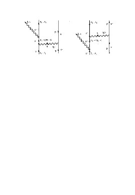
Figure 8: The Feynman diagrams contributing to radiative neutrino electron scattering via the charged current.

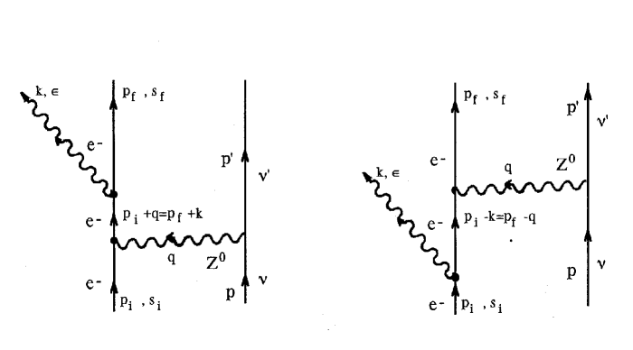
Figure 9: The Feynman diagrams contributing to radiative neutrino electron scattering via the neutral current.

The evaluation of the cross section associated with these diagrams is rather complicated, but in the present case the electrons are extremely non relativistic. Thus in the inverse of the (intermediate) electron propagator we can retain the mass rather than the momenta (exact results without this approximation will appear elsewhere). Then after some tedious, but straight-forward, trace calculations one can perform the angular integrals over the three-body final states to get:

$$k\frac{d\sigma(k,p_{e})}{dk}=\sigma_{\gamma}\frac{p_{e}dp_{e}}{m_{e}^{2}}[\rho+(1+\rho)\frac{p_{e}^{2}}{4E^{2}_{\nu}}]$$ (31)

where

$$\sigma_{\gamma}=\frac{37}{2\pi^{2}}(G_{F}~{}m_{e})^{2}~{}\alpha\approx 6.8\times 10^{-14}pb$$

sets the scale for this process, $\rho=5.4\times 10^{-2}$ is the ratio of the neutral to charged current contribution and $p_{e}$ is the final electron momentum. This momentum depends on the photon momentum k and the scattering angles. For a given $k$ is restricted as follows:

$$0\leq p_{e}\leq E_{\nu}-k$$

with maximum electron energy given by:

$$T_{e}=\frac{2(E_{\nu}-k)^{2}}{m_{e}}$$

From the above equations we cam immediately see that this process is roughly of order $\alpha$ down compared to the week neutrino-electron scattering cross-section. We also notice that the total cross section diverges logarithmically as the photon momentum goes to zero, reminiscent of the infrared divergence of Bremsstrahlung radiation. In our case we will adopt a lower photon momentum cutoff as imposed by our detector. We also notice that $\sigma_{\gamma}$, characterizing this process, is only a factor of three smaller than $\sigma_{0}$ characterizing the neutrino electron scattering cross section due to the magnetic moment. We should bare in mind, however, that:

1. The magnetic moment is not known. $\sigma_{0}$ was obtained with the rather optimistic value $\mu_{\nu}=10^{-12}\mu_{B}$, which is two orders of magnitude smaller than the present experimental limit.

2. One now has the advantage of observing not only the electron but the photon as well.

Integrating over the electron momenta we get

$$k\frac{d\sigma(k}{dk}=\sigma_{\gamma}~{}2\left[\frac{E_{\nu}-k}{m_{e}}\right]^{2}[\rho+2(1+\rho)\frac{(E_{\nu}-k)^{2}}{E^{2}_{\nu}}]$$ (32)

Integrating this cross-section with respect to the photon momentum we get:

$$\sigma_{total}=\sigma_{\gamma}~{}2\frac{E_{\nu}^{2}}{m^{2}_{e}}[(2+3\rho)\ell n\frac{E_{\nu}}{E_{cutoff}}-\frac{4+17\rho}{6}]$$ (33)

with the energy cutoff such lower than that required to make the above expression in the brackets vanish. Notice that the total cross-section is reduced further from the value $\sigma_{\gamma}$ by the ratio of the square of the neutrino energy divided by the electron mass.

We have considered in our discussion only electron targets. For such low energy neutrinos the charged current cannot operate on hadronic targets, since this process is not allowed so long as the target, being stable, is not capable of undergoing ordinary $\beta$ decay. The neutral current, however, can always make a contribution.

10 Summary and outlook

The perspective of the experiment is to provide high statistics -redundant, high precision measurement and minimize as much as possible the systematic uncertainties of experimental origin, which could be the main worry in the results of existing experiments. The physics goals of the new atmospheric neutrino measurement are summarized as follows:

1. Establish the phenomenon of neutrino oscillations with a different Experimental technique free of systematic biases. Thus one hopes to measure all the oscillation parameters, including the small mixing angle in the electronic neutrino, clarifying this way the nature of the oscillation mechanism.

2. A high sensitivity measurement of the neutrino magnetic moment, via electron neutrino scattering. At the same time radiative electron neutrino scattering will be investigated, exploiting the additional photon signature.

3. A new experimental investigation of neutrino decay.

4. Other novel improvements of the experimental sensitivity are possible and must be investigated. The benefit of increasing the gas pressure of the detector that increases proportionally the number of events must be investigated. A significant increase of event rate is a great step forward improving the experimental accuracy and reducing the impact of background rates.

11 Appendix

11.1 Modification of neutrino oscillations due to the magnetic moment

The electromagnetic interaction between the mass neutrino eigenstates $\nu_{i}$ and $\nu_{j}$ due to the magnetic moment $\mu_{ji}$ takes the form:

$$\textit{L}_{EM}=\mu_{ji}\bar{u}(p_{j})\sigma_{\lambda\rho}q^{\rho}u(p_{i})\epsilon^{\lambda}~{},~{}\mu_{ji}=10^{-12}\frac{\sqrt{4\pi\alpha}}{2m_{e}}(\frac{\mu_{ji}}{10^{-12}\mu_{B}})$$

with $\epsilon^{\lambda}$ the photon polarization and

$$\sigma_{\lambda\rho}=\frac{1}{2i}\left[\gamma_{\lambda},\gamma_{\rho}\right]~{}~{},~{}~{}q=p_{i}-p_{j}~{}~{}$$

For the moment will limit ourselves to the case of two generations only, i.e. we will ignore the small mixing $\delta$. The two cases of Dirac and Majorana neutrinos must be treated separately.

Majorana Neutrinos.

The flavor states are related to the mass eigenstates as follows:

$$\nu_{eL}=\cos{\theta}\nu_{1L}+\sin{\theta}\nu_{2L}$$

$$\nu_{\mu L}=-\sin{\theta}\nu_{1L}+\cos{\theta}\nu_{2L}$$

$$\nu_{eR}^{C}=\cos{\theta}\nu_{1R}+\sin{\theta}e^{i\alpha}\nu_{2R}$$

$$\nu_{\mu R}^{C}=-\sin{\theta}\nu_{1L}+\cos{\theta}e^{i\alpha}\nu_{2L}$$

In the above expressions for convenience we dropped the subscript ”solar” from the mixing angle. The above results are modified if the neutrinos have a magnetic moment and are found in a magnetic field. Then the left and the right neutrino fields are coupled via the dipole magnetic transition $\mu_{12}=\mu_{\nu}$. The diagonal elements of the magnetic transition operator (magnetic moments of the mass eigenstates) are zero (the Majorana neutrinos do not possess electromagnetic properties). Furthermore the magnetic moment submatrices are antisymmetric. Thus the mass eigenstates evolve as follows:

$\left(\begin{array}[]{c}\frac{d\nu_{1L}}{dt}\\ \frac{d\nu_{2L}}{dt}\\ \frac{d\nu_{1R}}{dt}\\ \frac{d\nu_{2R}}{dt}\\ \end{array}\right)=\left(\begin{array}[]{cccc}E_{1}&0&0&\mu_{\nu}B\\ 0&E_{2}&-\mu_{\nu}B&0\\ 0&-\mu_{\nu}B&E_{1}&0\\ \mu_{\nu}B&0&0&E_{2}\\ \end{array}\right)=\left(\begin{array}[]{c}\nu_{1L}\\ \nu_{2L}\\ \nu_{1R}\\ \nu_{2R}\end{array}\right)$
The eigenvalues of the above matrix are:

$$\lambda_{\pm}=\frac{E_{1}+E_{2}\pm\sqrt{(E_{1}-E_{2})^{2}+4(\mu_{\nu}B)^{2}}}{2}$$

(doubly degenerate), while the eigenvectors, indicated via $\eta_{1}^{+},\eta_{2}^{+},eta_{1}^{-},\eta_{2}^{-}$, are related to the mass eigenstates as follows:

$$\nu_{1L}=\sin{\theta_{1}}\eta_{1}^{+}+\cos{\theta_{1}}\eta_{1}^{-}$$

$$\nu_{2L}=\cos{\theta_{1}}\eta_{2}^{+}+\sin{\theta_{1}}\eta_{2}^{-}$$

$$\nu_{1R}=-\sin{\theta_{1}}\eta_{2}^{+}+\cos{\theta_{1}}\eta_{2}^{-}$$

$$\nu_{2R}=\cos{\theta_{1}}\eta_{1}^{+}-\sin{\theta_{1}}\eta_{1}^{-}$$

with the mixing angle defined by:

$$\tan{2\theta_{1}}=\frac{2\mu_{\nu}B}{E_{2}-E_{1}}=\frac{4\mu_{\nu}BE_{\nu}}{\Delta m_{21}^{2}}$$

Restricting oneself to two generations one now has the following pattern of neutrino oscillations:

$$P\left(\nu_{eL}\rightarrow\nu_{\mu L}\right)=\left[\cos{2\theta_{1}}\sin{2\theta}\sin{\pi\frac{L}{L_{21}}\sqrt{1+(\xi\frac{B}{1T})^{2}}}\right]^{2}$$

$$P\left(\nu_{eL}\rightarrow\nu^{C}_{eR}\right)=\sin^{2}{(\alpha/2)}\sin^{2}{2\theta_{1}}\left[\sin{\pi\frac{L}{L_{21}}\sqrt{1+(\xi\frac{B}{1T})^{2}}}\right]^{2}$$

$$P\left(\nu_{eL}\rightarrow\nu^{C}_{\mu R}\right)=\sin^{2}{2\theta_{1}}\sin^{2}{(\alpha/2)}\left[1-\sin{2\theta}\sin{\pi\frac{L}{L_{21}}\sqrt{1+(\xi\frac{B}{1T})^{2}}}\right]^{2}$$

$$P\left(\nu_{eL}\rightarrow\nu_{eL}\right)=1-\left[\sin{2\theta_{1}}+cos^{2}{2\theta_{1}}\sin^{2}{2\theta}\right]\sin^{2}{\pi\frac{L}{L_{21}}\sqrt{1+(\xi\frac{B}{1T})^{2}}}$$

with the parameter $\xi$ describes the mixing due to the neutrino magnetic moment, in a magnetic field taken to be of strength $1T$, and is given as follows:

$$\xi=\frac{4\mu_{\nu}E_{\nu}~{}1T}{\delta m^{2}_{21}}$$

We see that the oscillation $P\left(\nu_{eL}\rightarrow\nu^{C}_{eR}\right)$ vanishes when the relative $CP$ phase of the two eigenstates, $\alpha$, is zero, since, then, the flavor neutrinos are themselves Majorana particles. The electron neutrino disappearance probability in the three generation model discussed above takes the form:

$$P(\nu_{e}L\rightarrow\nu_{e}L)\approx 1 - \frac{\left[\sin^{2}{2\theta_{1}}^{2}+sin^{2}{2\theta}\cos^{2}{2\theta_{1}}\right]\sin^{2}{\pi\frac{L}{L_{21}}}\sqrt{1+(\xi\frac{B}{1T})^{2}}}{(1+\delta^{2})^{2}}$$ (34)

$$- \frac{4\delta^{2}\sin^{2}(\pi\frac{L}{L_{32}})}{(1+\delta^{2})^{2}}$$ (35)

We notice that the disappearance probability is independent of the phase $\alpha$. For $L_{12}>>L$, $L_{23}\approx L$ and for small magnetic moment the above equation becomes:

$$P\left(\nu_{eL}\rightarrow\nu_{eL}\right)\approx 1-\frac{\left[\sin{2\theta}^{2}+\xi^{2}(B/1T)^{2}\right](\pi\frac{L}{L_{21}})^{2}+4\delta^{2}\sin^{2}{\pi\frac{L}{L_{32}}}}{(1+\delta^{2})^{2}}$$ (36)

We see that in the experiment involving a triton target one will actually observe a sinusoidal oscillation as a function of the source-detector distance $L$ with an amplitude, which is proportional to the square of the small mixing angle $\delta$. The relevant oscillation length is given by:

$$L_{32}=2.476m\frac{E_{\nu}(MeV)}{\Delta m^{2}_{32}((eV)^{2})}$$

In the present experiment for an average neutrino energy $E_{\nu}\approx 15KeV$ and $\Delta m^{2}_{32}=2.5\times 10^{-3}(eV)^{2}$ we find

$$L_{32}\approx 15m$$

In other words the maximum will occur close to the source at about $L=7.5m$

Superimposed on this oscillation one will see an effect due to the smaller mass difference, which will increase quadratically with the distance $L$. In the presence of a magnetic field this will also depend quadratically in the magnetic field. The product of the mixing angle with the mass-squared difference in one hand and the effect of the magnetic moment squared are additive. This is indeed very beautiful experimental signature. Its practical exploitation depends, of course on the actual value of the parameter $\xi$. This can be cast in the form:

$$\xi=2\times 10^{-10}\frac{\mu_{\nu}}{10^{-12}\mu_{B}}\frac{E_{\nu}}{0.5MeV}\frac{10^{-2}~{}eV^{2}}{\delta m^{2}_{21}}$$ (37)

It is unfortunately clear that the parameter $\xi$ is unobservable in reactor experiments involving low energy neutrinos, even if the magnetic moment of the order of $10^{-12}\mu_{B}$. This is particularly true for the triton decay experiments with maximum energy of 18.6 KeV.

Dirac Neutrinos.

The case of Dirac neutrinos is not favored in most gauge theories. It is, however, a possibility favored in recent brane theories in extra dimensions. The flavor states are now related to the mass eigenstates as follows:

$$\nu_{eL}=\cos{\theta}\nu_{1L}+\sin{\theta}\nu_{2L}$$

$$\nu_{\mu L}=-\sin{\theta}\nu_{1L}+\cos{\theta}\nu_{2L}$$

$$\nu_{eR}=\cos{\theta}\nu_{1L}+\sin{\theta}\nu_{2L}$$

$$\nu_{\mu R}=-\sin{\theta}\nu_{1R}+\cos{\theta}e^{i\alpha}\nu_{2R}$$

The above results are also modified if the neutrinos have a magnetic moment and are found in a magnetic field. We will assume that, in the mass eigenstate basis, the off diagonal masses are much smaller than the off diagonal ones (GIM effect).We will consider the case of the inverse hierarchical masses, in which case in the masses $m_{1}$ and$m_{2}$ are almost degenerate. As a result the magnetic moments, which are proportional to the corresponding masses, are also almost equal. In this case the mass eigenstates evolve as follows:
$\left(\begin{array}[]{c}\frac{d\nu_{1L}}{dt}\\ \frac{d\nu_{2L}}{dt}\\ \frac{d\nu_{1R}}{dt}\\ \frac{d\nu_{2R}}{dt}\\ \end{array}\right)=\left(\begin{array}[]{cccc}E_{1}&0&\mu_{\nu}B&0\\ 0&E_{2}&0&\mu_{\nu}B\\ \mu_{\nu}B&0&E_{1}&0\\ 0&\mu_{\nu}B&0&E_{2}\\ \end{array}\right)=\left(\begin{array}[]{c}\nu_{1L}\\ \nu_{2L}\\ \nu_{1R}\\ \nu_{2R}\end{array}\right)$
The eigenvalues of the above matrix are:

$$\lambda_{1}=E_{1}+\mu_{\nu}B,\lambda_{2}=E_{1}-\mu_{\nu}B,\lambda_{3}=E_{2}+\mu_{\nu}B,\lambda_{4}=E_{2}-\mu_{\nu}B,$$

while the eigenvectors, indicated via $\eta_{1},\eta_{2},\eta_{3},\eta_{4}$, are related to the mass eigenstates as follows:

$$\nu_{1L}=\frac{1}{\sqrt{2}}(\eta_{1}+\eta_{2})$$

$$\nu_{2L}=\frac{1}{\sqrt{2}}(\eta_{3}+\eta_{4})$$

$$\nu_{1R}=\frac{1}{\sqrt{2}}(\eta_{1}-\eta_{2})$$

$$\nu_{2R}=\frac{1}{\sqrt{2}}(\eta_{3}-\eta_{4})$$

The following pattern of neutrino oscillations emerges:

$$P\left(\nu_{eL}\rightarrow\nu_{\mu L}\right)=\left[\cos{(\mu_{\nu}BL)}\sin{2\theta}\sin{\pi\frac{L}{L_{21}}}\right]^{2}$$

$$P\left(\nu_{eL}\rightarrow\nu_{eR}\right)=\sin^{2}{(\mu_{\nu}BL)}\left[1-\sin{2\theta}\sin{\pi\frac{L}{L_{21}}}\right]^{2}$$

$$P\left(\nu_{eL}\rightarrow\nu_{\mu R}\right)=\left[\sin{(\mu_{\nu}BL)}\sin{2\theta}\sin{\pi\frac{L}{L_{21}}}\right]^{2}$$

$$P\left(\nu_{eL}\rightarrow\nu_{eL}\right)=\cos^{2}{(\mu_{\nu}BL)}\left[1-\sin{2\theta}\sin{\pi\frac{L}{L_{21}}}\right]^{2}$$

The three generation electron neutrino disappearance probability takes the form:

$$P(\nu_{e}L\rightarrow\nu_{e}L)\approx 1-\frac{(\sin 2\theta)^{2}\sin^{2}{\pi\frac{L}{L_{21}}}\cos^{2}{(\mu_{\nu}BL)}-\sin^{2}{\mu_{(\nu}BL})+4\delta^{2}\sin^{2}{\pi\frac{L}{L_{32}}}}{(1+\delta^{2})^{2}}$$ (38)

For $L_{12}>>L$, $L_{23}\approx L$ and for small magnetic moment the above equation becomes:

$$P\left(\nu_{eL}\rightarrow\nu_{eL}\right)\approx 1-\frac{\left[\sin{2\theta}^{2}+\xi^{2}(B/1T)^{2}\right](\pi\frac{L}{L_{21}})^{2}+4\delta^{2}\sin^{2}{\pi\frac{L}{L_{32}}}}{(1+\delta^{2})^{2}}$$ (39)

We see that in this limit one cannot distinguish between the Dirac and Majorana neutrino oscillation patterns (compare eqs (36) and (39)).

11.2 Modification of neutrino oscillations due to decay

We will suppose the normal hierarchy of neutrino masses. In the presence of a finite neutrino decay width the quantum evolution of the neutrino mass eigenstate takes the form:

$$\nu_{i}(t)=\nu_{i}(0)Exp[-(iE_{i}+\Gamma_{i}/2)t]$$ (40)

where $\Gamma_{i},~{}i=2,3$ is the decay, width with respect to the laboratory, of $\nu_{i}$. The neutrino $\nu_{1}$ is assumed to be absolutely stable. The most common decay modes are VERGADOS :

$$\nu_{iL}\rightarrow\nu_{jL}+\gamma$$ (41)

radiative decay, which is expected to be quite slow. Or

$$\nu_{i}\rightarrow\nu_{j}+\nu_{k}+\bar{\nu}_{k}$$ (42)

which is also expected to be slow. One may also have

$$\nu_{iL}\rightarrow\nu_{jR}+\phi^{0}$$ (43)

which requires the existence of a very light physical Higgs scalar and sterile neutrinos. The most dominant mechanism is perhaps the Majoron emission:

$$\nu_{iL}\rightarrow\bar{\nu}_{jR}+\chi^{0}$$ (44)

available only to Majorana neutrinos.

In all the above channels the final neutrino $\nu_{j}$ is different from $\nu_{1}$ (in the case of processes (41) and (42) the final neutrino has a different energy, so it cannot be mistaken with $\nu_{1}$)

The widths $\Gamma_{k}=1/\tau_{k}$ can be related to those in the rest frame $\Gamma_{0k}=1/\tau_{0k}$ using the well known relation

$$\tau_{k}=\gamma\tau_{0k}=(E_{\nu_{e}}/m_{k})\tau_{0k}$$

The life-time in the rest frame can be cast in the form PAKVASA

$$\tau_{0}=\frac{1}{K_{0}}\frac{m_{i}}{m_{i}^{2}-m_{j}^{2}}(1+\frac{m_{j}}{m_{i}})^{-2}$$

We thus get

$$\Gamma_{i}=K_{0}\frac{m_{i}^{2}-m_{j}^{2}}{E_{\nu}}(1+\frac{m_{j}}{m_{i}})^{2}$$ (45)

The parameter $K_{0}$ depends on the model. For a lifetime for $\nu_{3}$ of the order of $10^{11}s$ we need $K_{0}$ of order of $10^{-10}$.

Since the neutrino $\nu_{1}$ can neither decay nor be repopulated, the relevant amplitude entering $\nu_{e}$ disappearance takes the form:

$$\cos^{2}{\theta}Exp[-iE_{1}]+\sin^{2}{\theta}Exp[-(iE_{2}+\Gamma_{2}/2)t]+\delta^{2}Exp[-(iE_{3}+\Gamma_{3}/2)t]$$

Thus the disappearance probability can be written as:

$$P(\nu_{e}L\rightarrow\nu_{e}L)=A^{2}(L)+B(L)-\frac{\sin^{2}2\theta\sin^{2}(\pi\frac{L}{L_{21}})+4\delta^{2}\sin^{2}(\pi\frac{L}{L_{32}})}{(1+\delta^{2})^{2}}$$ (46)

with $A(L)$ describing the part due to decay alone and $B(L)$ providing the collaborative effect due to oscillation and decay. One finds:

$$A(L)=1-\frac{\sin^{2}{\theta}[1-Exp(-\Gamma_{2}L/2)]+\delta^{2}[1-Exp(-\Gamma_{3}L/2)]}{1+\delta^{2}}$$ (47)

$$B(L) = \frac{\sin 2\theta^{2}\sin^{2}(\pi\frac{L}{L_{21}})[1-Exp(-\Gamma_{2}L/2)]}{(1+\delta^{2})^{2}}$$ (48)

$$+ \frac{4\delta^{2}\sin^{2}(\pi\frac{L}{L_{32}})\left[1-Exp(-\Gamma_{3}L/2)~{}[\cos^{2}{\theta}+\sin^{2}{\theta}Exp(-\Gamma_{2}L/2)]\ \right]}{(1+\delta^{2})^{2}}$$ (49)

In the absence of neutrino oscillations the disappearance is given by the function $A(L)$, which has the properties:

$$B(0)=0~{}~{},~{}~{}B(\infty)=\frac{\sin^{2}2\theta\sin^{2}(\pi\frac{L}{L_{21}})+4\delta^{2}\sin^{2}(\pi\frac{L}{L_{32}})}{(1+\delta^{2})}$$

$$A(0)=1~{}~{},~{}~{}A(\infty)=\frac{\cos^{4}{\theta_{solar}}}{(1+\delta^{2})^{2}}$$

In other words the neutrino oscillation is wiped out at sufficiently long distances.

11.3 Derivation of the neutrino decay width

We are now going to study the radiative neutrino decay, see (41), a bit further. The differential decay width for a neutrino $\nu_{i}$ with mass $m_{i}$ to a neutrino $\nu_{j}$ with mass $m_{j}$, $m_{i}>m_{j}$, with production of a photon of momentum $k$ is given by:

$$\frac{d\Gamma(i\rightarrow j)}{dk}=10^{-24}\frac{\alpha}{2}\frac{1}{(2m_{e})^{2}p_{i}}\left|\frac{\mu_{ij}}{10^{-12}\mu_{B}}\right|^{2}\frac{\left(m_{i}+m_{j}\right)^{4}}{m_{i}}$$ (50)

where $p_{i}$ is the momentum of the initial neutrino and the range of the photon momentum k is given by:

$$(1-\frac{m^{2}_{j}}{m^{2}_{i}})\frac{E_{i}-p_{i}}{2}\leq k\leq(1-\frac{m^{2}_{j}}{m^{2}_{i}})\frac{E_{i}+p_{i}}{2}$$

The total rate takes the form:

$$\Gamma(i\rightarrow j)=10^{-24}\frac{\alpha}{2}\frac{1}{(2m_{e})^{2}}\left|\frac{\mu_{ij}}{10^{-12}\mu_{B}}\right|^{2}(1-\frac{m^{2}_{j}}{m^{2}_{i}})\frac{\left(m_{i}+m_{j}\right)^{4}}{m_{i}}$$ (51)

The differential rate for electron neutrino disappearance takes the form

$$\frac{d\Gamma(\nu_{e}(E_{\nu})\rightarrow\nu_{e}(E_{\nu}-k))}{dk}=10^{-24}\sum_{j<i}\frac{\alpha}{2}\frac{1}{(2m_{e})^{2}2p_{i}}\left|\Lambda_{ij}\right|^{2}\frac{\left(m_{i}+m_{j}\right)^{4}}{m_{i}}$$ (52)

while the total rate takes the form:

$$\Gamma(\nu_{e}\rightarrow\nu_{e})=10^{-24}\sum_{j<i}\frac{\alpha}{2}\frac{1}{(2m_{e})^{2}}\left|\Lambda_{ij}\right|^{2}\frac{\left(m_{i}+m_{j}\right)^{4}}{m_{i}}(1-\frac{m^{2}_{j}}{m^{2}_{i}})$$ (53)

with

$$\Lambda_{ij}=U^{*}_{ej}U_{ei}\frac{\mu_{ij}}{10^{-12}\mu_{B}}$$

with the mass hierarchy $m_{j}<m_{i}$

References

-
(1)
See, e.g.
J.D. Vergados, Phys. Rep. 361, 1 (2002);
J.D. Vergados, Phys. Rep. 133, 1 (1986). - (2) P. Vogel and J.F. Beacon, Phys. Rev. D 60, 053003 (1999)
- (3) Y. Fukuda et al, The Super-Kamiokande Collaboration, Phys. Rev. Lett. 86, 5651 (2001); ibid 81, 1562 (1998); ibid 85, 3999 (2002).
-
(4)
Q.R. Ahmad et al, The SNO Collaboration, Phys. Rev.
Lett. 89 011302 (2002); ibid 89, 011301 (2002);
ibid 87 071301, (2001); ibid 89, 011301
(2002).
K. Lande et al, Homestake Collaboration, Astrophys, J 496, 505 (1998)
W. Hampel et al, The Gallex Collaboration, Phys. Lett. B 447 127, (1999);
J.N. Abdurashitov al, Sage Collaboration, Phys. Rev. c 80, 056801 (1999);
G.L Fogli et al, Phys. Rev. D 66, 053010 (2002) - (5) K. Eguchi et al, The KamLAND Collaboration, Submitted to Phys. Rev. Lett., hep-exp/0212021.
- (6) J,N. Bahcall, M.C. Gonzalez-Garcia, C. Pea-Garay, hep-ph/0212147
- (7) H Nunokawa et al, hep-ph/0212202.
- (8) P. Aliani et al, hep-ph/0212212.
- (9) V. Barger and D. Marfatia, hep-ph/0212126.
-
(10)
Y. Giomataris, Ph. Rebourgeant, J.P. Robert and C. Charpak,
Nucl. Instr. Meth Abf 376, 29 (1996);
J.I. Collar, Y. Giomataris, Nucl. Instr. Meth. A 471, 251 (2000)
J. Bouchez and Y. Giomataris, Private communication. - (11) P. Vogel and J. Engel, Phys. Rev. D 39, 3378 (1989).
- (12) J. Schechter and J.W.F. Valle, Phys. Rev. D 24, 1853 (1981); D 25, 283 (1982).
- (13) A.V. Derbin et al,Yad. Fiz. 57, 236 (1984); Phys. Atom. Nucl. 57, 222 (1994).
- (14) V.N. Trofimov et al,Yad. Fiz. 61, 1963 (1998); Phys. Atom. Nucl. 61, 1271 (1998).
- (15) T.L. Rashba, hep-ph/0104012.
- (16) V. Lobashev et al, Nuc. Phys. Proc. Sup. 91, 280 (2001)
- (17) KATRIN Collaboration, A. Osipowicz e͡t al, hep-exp/0109033
- (18) P. Gorodetzky et al., Nucl. Instr. and Meth. in Physics Research A 433, 554 (1999).
- (19) T. Ypsilantis, Europhys.News 27, 1996
- (20) [1b] G.Bonvicini, D.Naples, V.Paolone, Nucl.Instr.and Meth.A 491, 402 (2002).
- (21) [D.P. Snowden et al, Phys. Rev. D 61,01301 (2000);
- (22) http://www.unine.ch/phys/tpc.html
- (23) J. Bouchez, I. Giomataris, DAPNIA-01-07, Jun 2001
- (24) M. Ichige et al., Nucl.Instrum. Meth. A 333, 355 (1993)
- (25) [R. Luscher et al, Nucl. Phys. Proc. Suppl. 95, 233 (2001)2001
- (26) ICARUS Collaboration, Nucl. Instr. And Meth. A 356, 256 (1994).
- (27) K.Zioutas et al, Nucl. Instr. and Meth. A 425, 480 (1999).
- (28) C.E. Aalseth et al, Nucl. Phys. Proc. Suppl. 110, :85 (2002)
- (29) A. Magnon et al, Nucl. Instr. Meth. A 478, 210 (2002)
- (30) S. Andriamonje et al, DAPNIA-02-47, Submitted to Nucl. Phys. B
- (31) I. Giomataris , Nucl. Instr. Meth. A 419 , 239 (1998).
- (32) J. Derre et al, Nucl. Instr. Meth. A 449, 554 (1999).
- (33) J. Derre e͡t al, Nucl. Instr. Meth. A 449, 523 (2001).
- (34) B.S.Neganov et al., Phys. Atom. Nucl.,Vol.64,No.11, 1948 (2001).
-
(35)
D. Indumathi, hep-ph/0212038;
A. Bandyopadhyay, S. Choubey and S. Goswami, Phys. Rev. D 65, 073021 (2002);
A. Bandyopadhyay, S. Choubey and S. Goswami, hep-ph/0204173. - (36) A. Acker and S. Pakvasa, Phys. Lett. B 320, 320 (1994); hep-ph/9320207.
-
(37)
Y. Chikashige, R.N. Mohapatra and R.D. Peccei, Phys. Lett. 98 B, 265 (1981)
G.B. Gelmini and M. Rocandelli Phys. Lett. 99 B, 411 (1981) - (38) J.F. Beacom and N.F. Bell, Phys. Rev. D 65, 113009 (2002); hep-ph/0204111.
-
(39)
C.W. Kim and W.P. Lam, Mod. Phys. Lett. A 5, 297 (1990);
C. Kiunti, C.W. Kim, U.W. Lee and W.P. Lam,Phys. Rev. D 45, 1557 (1992);
Z.G. Berezhiani, G. Fiorentini, M. Moretti and A. Rossi, Z. Phys. C 54, 581 (1992).