The BABAR Collaboration

Using events in which one of two neutral $B$ mesons from the decay of an $\mathchar 28935\relax{(4S)}$ resonance is fully reconstructed, we set limits on the lifetime difference between the two neutral-$B$ mass eigenstates and on $C\!P$, $T$, and $C\!PT$ violation in $B^{0}{\kern-1.60004pt\kern 1.79993pt\overline{\kern-1.79993ptB}{}^{0}}$ mixing. Both $C\!P$ and non-$C\!P$ eigenstates were obtained from the 88 million $\mathchar 28935\relax{(4S)}\rightarrow B\kern 1.79993pt\overline{\kern-1.79993ptB}{}$ decays collected between 1999 and 2002 with the BABAR detector at the PEP-II asymmetric-energy $B$-Factory at SLAC. We determine six independent parameters governing mixing ($\Delta m$, $\Delta\Gamma/\Gamma$), $C\!PT$/$C\!P$ violation (${\mathop{\rm Re}}z$, ${\mathop{\rm Im}}z$), and $C\!P$/$T$ violation (${\mathop{\rm Im}}\lambda_{C\!P}$, $|q/p|$), where $\lambda_{C\!P}$ characterizes $B^{0}$ and $\kern 1.79993pt\overline{\kern-1.79993ptB}{}^{0}$ decays to states of charmonium plus $K^{0}_{\scriptscriptstyle S}$ or $K^{0}_{\scriptscriptstyle L}$. The preliminary results are

$$\begin{array}[]{ r@{\ \ =\ }r@{.}l@{\pm 0.}l@{{\rm(stat.)}\pm 0.} l@{{\rm{(syst.)}}\ \ [}r@{,}l@{]}l}\mathop{\rm{sgn}}({\mathop{\rm Re}}\lambda_{C\!P})\Delta\Gamma/\Gamma&-0&008&037&018&-0.084&0.068&~{},\\ |q/p|&1&029&013&011&1.001&1.057&~{},\\ \left({\mathop{\rm Re}}\lambda_{C\!P}/|\lambda_{C\!P}|\right){\mathop{\rm Re}}z&0&014&035&034&-0.072&0.101&~{},\\ {\mathop{\rm Im}}z&0&038&029&025&-0.028&0.104&~{}.\end{array}$$

The values inside square brackets indicate the 90% confidence-level intervals. For ${\mathop{\rm Im}}\lambda_{C\!P}/|\lambda_{C\!P}|$ and $\Delta m$ we find values consistent with recent results from other analyses. These results are consistent with Standard Model expectations.

1 Introduction and analysis overview

The neutral $B^{0}_{d}$ meson system has two mass eigenstates with mass and total decay rate differences $\Delta m$ and $\Delta\Gamma$. While the mass difference has been measured recently with high precision [1, 2, 3, 4], only weak limits exist for the lifetime difference $\Delta\tau_{B}=-\Delta\Gamma/\Gamma^{2}$. Using the time-integrated mixing parameter $\chi_{d}$, the CLEO Collaboration has set a limit of $|\Delta\Gamma/\Gamma|<80\%$ [6]. A stronger constraint, $|\Delta\Gamma/\Gamma|<20\%$ at 90% confidence-level, has been obtained by the DELPHI Collaboration from a direct time-dependent study using flavor eigenstate events [7]. In the Standard Model, the ratio of the difference in the decay widths to the difference of the masses is proportional to $m_{b}^{2}/m_{t}^{2}$ and thus quite small. Recent calculations of $\Delta\Gamma/\Gamma$, including $1/m_{b}$ contributions and part of the next-to-leading order QCD corrections within the Standard Model [5], find values of about $-0.3\%$. The large data set available at the asymmetric $B$ Factories provides the opportunity to reach much closer to the anticipated range for $\Delta\Gamma/\Gamma$.

The behavior of neutral $B$ mesons is sensitive to $C\!PT$ violation [8, 9]. The $C\!PT$ theorem [10, 11], based on very general principles of relativistic quantum field theory, states that the triple product of the universal discrete symmetries $C$, $P$, and $T$ represent an exact symmetry. The $C\!PT$ symmetry remains to date the only combination of $C$, $P$, and $T$ that is not known to be violated. However, the proof of the $C\!PT$ theorem relies on locality, which could break down at very short distances. For instance, string theories are fundamentally non-local and therefore do not necessarily fulfill the conditions of the $C\!PT$ theorem. Therefore it is possible, although perhaps unlikely, that $C\!PT$ could break down. To date, the best tests have come from experiments in the neutral kaon system [12]. Bounds obtained so far in the $B$ meson system [4, 13] are, however, mainly sensitive to the absorptive (lifetime) component of the Hamiltonian, where the small expected value of $\Delta\Gamma$ suppresses the asymmetry effects.

Violation of $C\!P$ in the neutral $B$ meson system may occur in mixing, in decay, or in the interference between mixing and decay. There is no fundamental way of assigning the source of $C\!P$ violation observed in interference to either mixing or to decay. The standard phase choice puts $C\!P$ violation in the mixing, but this is simply a convention. Other observable processes, however, can isolate $C\!P$ violation due entirely to mixing. Similarly, mixing may intrinsically contain $T$ violation or even $C\!PT$ violation. It is these possibilities for the breaking of discrete symmetries in mixing itself that we address in this analysis.

To measure the lifetime difference of the neutral $B$-meson mass eigenstates and $C\!P$, $T$, or $C\!PT$ violation we observe the time dependence of decays of neutral $B$ mesons produced in pairs at the $\mathchar 28935\relax{(4S)}$ resonance. The conventional mixing and $C\!P$ analyses allow for exponential decay modulated by oscillatory terms with frequency $\Delta m$. This neglects the difference between the decay rates $\Delta\Gamma$ of the two mass eigenstates, which would introduce new exponential factors. $C\!P$, $T$, and $C\!PT$ violation in the mixing of the neutral $B$ mesons would modify the coefficients of the various terms involving exponential and oscillatory behavior. To detect these potential subtle changes requires precision measurements of the decays and thorough consideration of systematic issues. It also requires a more comprehensive treatment of the coherent decays of the mesons than has been conducted previously.

The analysis is based on a total of about 88 million $\mathchar 28935\relax{(4S)}\rightarrow B\kern 1.79993pt\overline{\kern-1.79993ptB}{}$ decays collected between 1999 and 2002 with the BABAR detector at the PEP-II asymmetric-energy $B$ Factory at the Stanford Linear Accelerator Center. There, 9 $\mathrm{\,Ge\kern-1.00006ptV}$ electrons and 3.1 $\mathrm{\,Ge\kern-1.00006ptV}$ positrons annihilate to produce the $B\kern 1.79993pt\overline{\kern-1.79993ptB}{}$ pairs moving along the $e^{-}$ beam direction ($z$-axis) with a Lorentz boost of $\beta\gamma\approx 0.56$, allowing a measurement of the proper time difference $\Delta t$ between the two $B$ decays. In this analysis, one $B$ meson is fully reconstructed in a flavor ($B_{\rm flav}$) or $C\!P$ ($B_{C\!P}$) eigenstate (generally denoted as $B_{\rm rec}$). The remaining charged particles in the event, which originate from the other $B$ meson ($B_{\rm tag}$), are used to identify its flavor as $B^{0}$ or $\kern 1.79993pt\overline{\kern-1.79993ptB}{}^{0}$. The time difference $\Delta t=t_{\rm rec}-t_{\rm tag}\approx\Delta z/\beta\gamma c$ is determined from the separation $\Delta z$ of the decay vertices for the fully reconstructed $B$ candidate and the tagging $B$ along the boost direction.

A single maximum-likelihood fit to the time distributions of tagged and untagged, flavor and $C\!P$ eigenstates determines six independent parameters (see Sec. 2) governing mixing ($\Delta m$, $\Delta\Gamma/\Gamma$), $C\!PT$/$C\!P$ violation (${\mathop{\rm Re}}z$, ${\mathop{\rm Im}}z$) and $C\!P$/$T$ violation (${\mathop{\rm Im}}\lambda_{C\!P}$, $|q/p|$), where $\lambda_{C\!P}$ is the traditional variable characterizing the decays of neutral $B$ mesons into final states of charmonium and a $K^{0}_{\scriptscriptstyle S}$ or $K^{0}_{\scriptscriptstyle L}$. The parameters ${\mathop{\rm Im}}\lambda_{C\!P}$ and $\Delta m$ are used only as a cross-check with the BABAR $\sin 2\beta$ analysis [14] and previous $\Delta m$ results [1, 2, 3, 4].

The analysis has several challenges. First, the tagged $B$ and the fully reconstructed $B$ decays are correlated and interference between allowed and doubly-$\rm CKM$-suppressed (DCKM) decays cannot be neglected. Second, tagging incorrectly assigns the flavor with a certain mistag probability. Third, the resolution for $\Delta t$ is comparable to the $B$ lifetime and asymmetric for positive and negative $\Delta t$. This asymmetry must be well understood lest it be mistaken for a fundamental asymmetry we seek to measure. Fourth, possible direct $C\!P$ violation in the $B_{C\!P}$ sample can be a competing source of fake effects and must be parameterized appropriately. Finally, we have to account possible asymmetries induced by the differing response of the detector to positive and negative particles. In resolving these issues we rely mainly on data.

The paper is organized as follows. In Sec. 2 we present a general formulation of the time-dependent decay rates of $B^{0}{\kern-1.60004pt\kern 1.79993pt\overline{\kern-1.79993ptB}{}^{0}}$ pairs produced at the $\mathchar 28935\relax{(4S)}$ resonance, including effects from the lifetime difference, possible $C\!PT$ violation, and interference effects induced by doubly-$\rm CKM$-suppressed decays. We derive the expressions for $B$ decays to final states with flavor and $C\!P$ eigenstates. In Sec. 3 we describe the BABAR detector. After discussing the data sample in Sec. 4, we describe the $b$-quark tagging algorithm in Sec. 5. Sec. 6 is devoted to the description of the measurement of ${\rm\Delta}z$ and the determination of $\Delta t$ and its resolution function. In Sec. 7 we describe the unbinned log-likelihood function and the assumptions made in the nominal fit. The results of the fit are given in Sec. 8. Cross-checks are discussed in Sec. 9 and systematic uncertainties are summarized in Sec. 10. The results of the analysis are summarized and discussed in Sec. 11.

2 General time-dependent decay rates from $\mathchar 28935\relax(4S)\rightarrow B^{0}{\kern-1.60004pt\kern 1.79993pt\overline{\kern-1.79993ptB}{}^{0}}$

The neutral $B$ meson system can be described by the effective Hamiltonian $\tilde{M}-i\tilde{\Gamma}/2$, where ${\tilde{M}}$ and ${\tilde{\Gamma}}$ are two-by-two hermitian matrices describing, respectively, the mass (dispersive) and lifetime (absorptive) components. If either $C\!P$ or $C\!PT$ is a good symmetry, then $M_{11}=M_{22}$ and $\Gamma_{11}=\Gamma_{22}$, with the index $1$ indicating $B^{0}$  and $2$ indicating $\kern 1.79993pt\overline{\kern-1.79993ptB}{}^{0}$. If either $C\!P$ or $T$ is a good symmetry, $\Gamma_{12}/M_{12}$ is real. This condition does not depend on the phase convention chosen for the $B^{0}$ and $\kern 1.79993pt\overline{\kern-1.79993ptB}{}^{0}$. The masses $\mu_{\pm}$ and decay rates $\gamma_{\pm}$ of the two eigenstates are

$$\omega_{\pm}=\mu_{\pm}-\frac{i}{2}\gamma_{\pm}=M-\frac{i}{2}\Gamma\pm\sqrt{\left(M_{12}-\frac{i}{2}\Gamma_{12}\right)\left(M_{12}^{*}-\frac{i}{2}\Gamma_{12}^{*}\right)+\left(\delta M-\frac{i}{2}\delta\Gamma\right)^{2}}~{},$$ (1)

where we define

$$M\equiv\frac{M_{11}+M_{22}}{2}\quad,\quad\Gamma\equiv\frac{\Gamma_{11}+\Gamma_{22}}{2}\quad,\quad\delta M\equiv\frac{M_{11}-M_{22}}{2}\quad,\quad\delta\Gamma\equiv\frac{\Gamma_{11}-\Gamma_{22}}{2}~{}.$$ (2)

Neglecting $C\!PT$ violation, and anticipating that the lifetime difference is small compared to the mass difference, we have

$$\Delta m=2|M_{12}|~{};\qquad\Delta\Gamma=2|M_{12}|{\mathop{\rm Re}}(\Gamma_{12}/M_{12})~{}.$$ (3)

Here we have taken $\Delta m$ to be the mass of the heavier state minus the mass of the lighter. Thus $\Delta\Gamma$ is the decay rate of the heavier state minus the decay rate of the lighter and its sign is not known a priori.

The light and heavy mass eigenstates of the neutral $B$-meson system may be written

$$|B_{L}\rangle = p|B^{0}\rangle+q|\kern 1.79993pt\overline{\kern-1.79993ptB}{}^{0}\rangle$$

$$|B_{H}\rangle = p|B^{0}\rangle-q|\kern 1.79993pt\overline{\kern-1.79993ptB}{}^{0}\rangle$$ (4)

where

$${q\over p}\equiv-\sqrt{{M^{\ast}_{12}-\frac{i}{2}\,\Gamma^{\ast}_{12}\over M_{12}-\frac{i}{2}\,\Gamma_{12}}}~{}.$$ (5)

The magnitude of $q/p$ is very nearly unity:

$$\left|\frac{q}{p}\right|^{2}\approx 1-{\mathop{\rm Im}}\frac{\Gamma_{12}}{M_{12}}~{}.$$ (6)

In the Standard Model, the $C\!P$- and $T$-violating quantity $|q/p|^{2}-1$ is small not just because $|\Gamma_{12}|$ is small, but additionally because the $C\!P$-violating quantity ${\mathop{\rm Im}}(\Gamma_{12}/M_{12})$ would vanish if the $u$- and $c$-quark mass were the same. $C\!P$ violation is not possible in mixing if two of the quark masses (for quarks of identical charge) are identical because we could redefine them so one quark did not mix with the other two. The remaining two generations would be inadequate to support $C\!P$ violation. The result is that ${\mathop{\rm Im}}(\Gamma_{12}/M_{12})$ is suppressed by an additional factor $m_{c}^{2}/m_{b}^{2}\approx 0.1$. When the remaining factors are included, the result is $|{\mathop{\rm Im}}({\Gamma_{12}}/{M_{12}})|<10^{-3}$.

$C\!PT$ violation in mixing can be described conveniently by the phase-convention independent quantity

$$z\equiv{\delta M-\frac{i}{2}\,\delta\Gamma\over\sqrt{\left(M_{12}-\frac{i}{2}\,\Gamma_{12}\right)\left(M^{\ast}_{12}-\frac{i}{2}\,\Gamma^{\ast}_{12}\right)+\left(\delta M-\frac{i}{2}\,\delta\Gamma\right)^{2}}}~{}=~{}\frac{\delta M-\frac{i}{2}\,\delta\Gamma}{\frac{1}{2}\left(\Delta m-\frac{i}{2}\Delta\Gamma\right)}~{}.$$ (7)

States that begin as purely $B^{0}$ or $\kern 1.79993pt\overline{\kern-1.79993ptB}{}^{0}$  will oscillate and after a time $t$ will be mixtures

$$\begin{split}|{{B^{0}}_{\text{phys}}(t)}\rangle&=\bigl{(}g_{+}(t)+z\cdot g_{-}(t)\bigr{)}\,|{B^{0}}\rangle-\sqrt{1-z^{2}}\cdot\frac{q}{p}\,g_{-}(t)\,|{\kern 1.79993pt\overline{\kern-1.79993ptB}{}^{0}}\rangle\\ |{{\kern 1.79993pt\overline{\kern-1.79993ptB}{}^{0}}_{\text{phys}}(t)}\rangle&=\bigl{(}g_{+}(t)-z\cdot g_{-}(t)\bigr{)}\,|{\kern 1.79993pt\overline{\kern-1.79993ptB}{}^{0}}\rangle-\sqrt{1-z^{2}}\cdot\frac{p}{q}\,g_{-}(t)\,|{B^{0}}\rangle~{},\end{split}$$ (8)

where we have introduced

$$g_{\pm}(t)=\frac{1}{2}(e^{-i\omega_{+}t}\pm e^{-i\omega_{-}t})~{}.$$ (9)

At the $\mathchar 28935\relax(4S)$ resonance, neutral $B$ mesons are produced in coherent pairs. If we subsequently observe a final state $f_{1}$ at time $t_{0}=0$ and another state $f_{2}$ at some other time $t$, either positive or negative, we cannot in general know whether $f_{1}$ came from the decay of a $B^{0}$ or a $\kern 1.79993pt\overline{\kern-1.79993ptB}{}^{0}$   and similarly for the state $f_{2}$. If $A_{1,2}$ and ${\overline{A}}_{1,2}$ are the amplitudes for the decay of $B^{0}$ and $\kern 1.79993pt\overline{\kern-1.79993ptB}{}^{0}$ to the states $f_{1}$ and $f_{2}$, then the overall amplitude when $t>0$ is given by

$${\cal A} = a_{+}g_{+}(t)+a_{-}g_{-}(t)~{},$$ (10)

where

$$a_{+} = -A_{1}{\overline{A}}_{2}+{\overline{A}}_{1}A_{2}$$

$$a_{-} = \sqrt{1-z^{2}}\left[{p\over q}A_{1}A_{2}-{q\over p}{\overline{A}}_{1}{\overline{A}}_{2}\right]+z[A_{1}{\overline{A}}_{2}+{\overline{A}}_{1}A_{2}]~{}.$$ (11)

Using the relations

$$|g_{\pm}(t)|^{2}=\frac{1}{2}\,e^{-t/\tau_{B}}\left[\cosh(\Delta\Gamma t/2)\pm\cos(\Delta mt)\right]$$ (12)

and

$$g_{+}^{\ast}(t)\,g_{-}(t)=-\frac{1}{2}\,e^{-t/\tau_{B}}\left[\sinh(\Delta\Gamma t/2)+i\,\sin(\Delta mt)\right]~{},$$ (13)

with $\tau_{B}=1/\Gamma$, we find the decay rate, which in fact is correct for $t$ positive or negative,

$${{\rm d}N\over{\rm d}t}\propto e^{-\Gamma|t|}\Bigl{\{}{1\over 2}c_{+}\cosh(\Delta\Gamma t/2)+{1\over 2}c_{-}\cos(\Delta mt)-{\mathop{\rm Re}}\,s\,\sinh(\Delta\Gamma t/2)+{\mathop{\rm Im}}\,s\,\sin(\Delta mt)\Bigr{\}}$$ (14)

where

$$c_{\pm}=|a_{+}|^{2}\pm|a_{-}|^{2}~{};\quad s=a_{+}^{*}a_{-}~{}.$$ (15)

Now let us take $f_{1}\equiv f_{tag}$ to be the state that is incompletely reconstructed and which provides the tagging decay, and $f_{2}\equiv f_{rec}$ the fully reconstructed state (flavor or $C\!P$ eigenstate). Because the tagging algorithm is imperfect, we may incorrectly identify the flavor of the decaying $B$ meson. This can be accounted for by incoherently combining correct and incorrect tags. A more subtle problem arises because there may be a basic ambiguity: the state $f_{tag}$ may result from interference between decay from a $B^{0}$ and decay from a $\kern 1.79993pt\overline{\kern-1.79993ptB}{}^{0}$. We consider first the simpler situation where there is no underlying ambiguity.

If the tag is a $\kern 1.79993pt\overline{\kern-1.79993ptB}{}^{0}$, we display this explicitly writing ${\overline{A}}_{{\overline{tag}}}\neq 0,A_{{\overline{tag}}}=0$. We define

$$\lambda_{rec}=\frac{q}{p}\frac{\overline{A}_{rec}}{A_{rec}}~{},$$ (16)

which is independent of phase conventions for the $B^{0}$ and $\kern 1.79993pt\overline{\kern-1.79993ptB}{}^{0}$ states. Dropping terms of order $z^{2}$, we find a decay rate

$${{\rm d}N\over{\rm d}t}{(tag=\kern 1.79993pt\overline{\kern-1.79993ptB}{}^{0})} \!\propto\! |{\overline{A}}_{\rm\overline{tag}}|^{2}|A_{rec}|^{2}e^{-\Gamma|t|}\Biggl{\{}{1\over 2}\left[1+|\lambda_{rec}-z|^{2}\right]\cosh(\Delta\Gamma t/2)$$ (17)

$$\qquad+{1\over 2}\left[1-|\lambda_{rec}-z|^{2}\right]\cos(\Delta mt)$$

$$\qquad-{\mathop{\rm Re}}(-\lambda_{rec}+z)\sinh(\Delta\Gamma t/2)+{\mathop{\rm Im}}(-\lambda_{rec}+z)\sin(\Delta mt)\Biggr{\}}~{}.$$

Correspondingly, if $f_{tag}$ is tagged as a $B^{0}$, ${\overline{A}}_{tag}=0,\ A_{tag}\neq 0$, and we have

$${{\rm d}N\over{\rm d}t}{(tag=B^{0})} \!\propto\! |{A}_{\rm tag}|^{2}|A_{rec}|^{2}\left|\frac{p}{q}\right|^{2}e^{-\Gamma|t|}\Biggl{\{}{1\over 2}\left[|\lambda_{rec}|^{2}+|1+z\lambda_{rec}|^{2}\right]\cosh(\Delta\Gamma t/2)$$

$$\qquad+{1\over 2}\left[|\lambda_{rec}|^{2}-|1+z\lambda_{rec}|^{2}\right]\cos(\Delta mt)$$

$$\qquad+{\mathop{\rm Re}}[\lambda_{rec}^{*}(1+\lambda_{rec}z)]\sinh(\Delta\Gamma t/2)-{\mathop{\rm Im}}[\lambda_{rec}^{*}(1+\lambda_{rec}z)]\sin(\Delta mt)\Biggr{\}}~{}.$$

The normalizations are identical in Eqs. (17) and (LABEL:eq:btag_general).

We consider several scenarios. If $f_{rec}$ is a $C\!P$ eigenstate, then $|\lambda_{C\!P}|=R_{C\!P}|q/p|$, with $R_{C\!P}=|\overline{A}_{C\!P}/A_{C\!P}|$. If all the weak decay mechanisms have the same weak phase, $R_{C\!P}=1$. This is expected for final states like ${J\mskip-3.0mu/\mskip-2.0mu\psi\mskip 2.0mu}K^{0}_{\scriptscriptstyle S}$, where indeed measurements show $|\lambda_{C\!P}|\approx 1$ [14]. Dropping quadratic terms in $z$ and $\Delta\Gamma$ we have

$${{\rm d}N\over{\rm d}t}{(tag=\kern 1.79993pt\overline{\kern-1.79993ptB}{}^{0};rec=C\!P)} \!\propto\! |{\overline{A}}_{\rm\overline{tag}}|^{2}|A_{C\!P}|^{2}e^{-\Gamma|t|}\Biggl{\{}{1\over 2}\left[1+|\lambda_{C\!P}|^{2}-2{\mathop{\rm Re}}\lambda_{C\!P}{\mathop{\rm Re}}z-2{\mathop{\rm Im}}\lambda_{C\!P}{\mathop{\rm Im}}z\right]$$ (19)

$$\qquad+{1\over 2}\left[1-|\lambda_{C\!P}|^{2}+2{\mathop{\rm Re}}\lambda_{C\!P}{\mathop{\rm Re}}z+2{\mathop{\rm Im}}\lambda_{C\!P}{\mathop{\rm Im}}z\right]\cos(\Delta mt)$$

$$\qquad+{\mathop{\rm Re}}\lambda_{C\!P}\sinh(\Delta\Gamma t/2)-{\mathop{\rm Im}}\left[\lambda_{C\!P}-z\right]\sin(\Delta mt)\Biggr{\}}~{},$$

$${{\rm d}N\over{\rm d}t}{(tag=B^{0};rec={C\!P})} \!\propto\! |{A}_{\rm tag}|^{2}|A_{C\!P}|^{2}\left|\frac{p}{q}\right|^{2}e^{-\Gamma|t|}\Biggl{\{}{1\over 2}\left[1+|\lambda_{C\!P}|^{2}+2{\mathop{\rm Re}}\lambda_{C\!P}{\mathop{\rm Re}}z-2{\mathop{\rm Im}}\lambda_{C\!P}{\mathop{\rm Im}}z\right]$$ (20)

$$\qquad+{1\over 2}\left[|\lambda_{C\!P}|^{2}-1-2{\mathop{\rm Re}}\lambda_{C\!P}{\mathop{\rm Re}}z+2{\mathop{\rm Im}}\lambda_{C\!P}{\mathop{\rm Im}}z\right]\cos(\Delta mt)$$

$$\qquad+{\mathop{\rm Re}}\lambda_{C\!P}\sinh(\Delta\Gamma t/2)+{\mathop{\rm Im}}\left[\lambda_{C\!P}-|\lambda_{C\!P}|^{2}z\right]\sin(\Delta mt)\Biggr{\}}~{}.$$

Data from directly related final states like ${J\mskip-3.0mu/\mskip-2.0mu\psi\mskip 2.0mu}K^{0}_{\scriptscriptstyle S}$, with $\eta_{C\!P}=-1$, and ${J\mskip-3.0mu/\mskip-2.0mu\psi\mskip 2.0mu}K^{0}_{\scriptscriptstyle L}$, with $\eta_{C\!P}=+1$, where $\eta_{C\!P}$ is the $C\!P$ eigenvalue of the final state, can be combined by assuming that they are identical, except for an overall sign in $\lambda_{C\!P}$.

We assume that the decays of flavor eigenstates are dominated by a single weak mechanism, so that $|A_{\rm flav}|=|{\overline{A}}_{{\overline{\rm flav}}}|$, $|{\overline{A}}_{\rm flav}|=|{A}_{{\overline{\rm flav}}}|$. This will enable us to relate the four possibilities that arise from the tag and reconstructed state being either $B^{0}$ or $\kern 1.79993pt\overline{\kern-1.79993ptB}{}^{0}$. When the fully reconstructed meson $f_{rec}$ is a flavor eigenstate, $|\lambda_{rec}|$ is either very small or very large. If it appears to come from a $B^{0}$, then $|\lambda_{\rm flav}|\ll 1$ and we have

$${{\rm d}N\over{\rm d}t}{(tag=\kern 1.79993pt\overline{\kern-1.79993ptB}{}^{0};rec=B^{0})} \!\propto\! |{A}_{\rm{tag}}|^{2}|A_{{\rm flav}}|^{2}e^{-\Gamma|t|}\Biggl{\{}{1\over 2}+{1\over 2}\cos(\Delta mt)+{\mathop{\rm Im}}(-\lambda_{\rm flav}+z)\sin(\Delta mt)\Biggr{\}}~{},$$

$${{\rm d}N\over{\rm d}t}{(tag=B^{0};rec=B^{0})} \!\propto\! |{A}_{\rm tag}|^{2}|A_{\rm flav}|^{2}\left|\frac{p}{q}\right|^{2}e^{-\Gamma|t|}\Biggl{\{}{1\over 2}-{1\over 2}\cos(\Delta mt)+{\mathop{\rm Im}}\lambda_{\rm flav}\sin(\Delta mt)\Biggr{\}}~{}.$$

Conversely, if the fully reconstructed state is nominally a $\kern 1.79993pt\overline{\kern-1.79993ptB}{}^{0}$, $|\lambda_{\overline{\rm flav}}|\gg 1$ and

$${{\rm d}N\over{\rm d}t}{(tag=\kern 1.79993pt\overline{\kern-1.79993ptB}{}^{0};rec=\kern 1.79993pt\overline{\kern-1.79993ptB}{}^{0})} \!\propto\! |{A}_{\rm{tag}}|^{2}|{A}_{\rm\overline{flav}}|^{2}|\lambda_{\overline{\rm flav}}|^{2}e^{-\Gamma|t|}\Biggl{\{}{1\over 2}-{1\over 2}\cos(\Delta mt)+{\mathop{\rm Im}}\overline{\lambda}_{\rm flav}\sin(\Delta mt)\Biggr{\}}$$

$$\!\propto\! |{A}_{\rm{tag}}|^{2}|A_{\rm flav}|^{2}\left|\frac{q}{p}\right|^{2}e^{-\Gamma|t|}\Biggl{\{}{1\over 2}-{1\over 2}\cos(\Delta mt)+{\mathop{\rm Im}}\overline{\lambda}_{\rm flav}\sin(\Delta mt)\Biggr{\}}~{},$$

(23)

$${{\rm d}N\over{\rm d}t}{(tag=B^{0};rec=\kern 1.79993pt\overline{\kern-1.79993ptB}{}^{0})} \!\propto\! |{A}_{\rm tag}|^{2}|{A}_{\rm\overline{flav}}|^{2}\left|\frac{p}{q}\right|^{2}|\lambda_{\overline{\rm flav}}|^{2}e^{-\Gamma|t|}\Biggl{\{}{1\over 2}+{1\over 2}\cos(\Delta mt)$$

$$\qquad-{\mathop{\rm Im}}[z+\overline{\lambda}_{\rm flav}]\sin(\Delta mt)\Biggr{\}}$$

$$\!\propto\! |{A}_{\rm tag}|^{2}|{A}_{\rm{flav}}|^{2}e^{-\Gamma|t|}\Biggl{\{}{1\over 2}+{1\over 2}\cos(\Delta mt)-{\mathop{\rm Im}}[z+\overline{\lambda}_{\rm flav}]\sin(\Delta mt)\Biggr{\}}~{},$$

where $\overline{\lambda}_{\rm flav}\equiv 1/\lambda_{\overline{\rm flav}}$. We see that the overall normalization in the mixed final states has a factor of $|q/p|^{2}$ or $|p/q|^{2}$ relative to the unmixed final states.

Doubly-$\rm CKM$-suppressed decays, such as $B^{0}\rightarrow D^{+}\pi^{-}$, occur at a rate roughly $|V_{ub}^{*}V_{cd}/V_{cb}^{*}V_{ud}|^{2}\approx(0.02)^{2}$, and can be ignored. However, interference between favored and suppressed decays are reduced by a factor of approximately $0.02$. For decays reconstructed in a final state as apparent $B^{0}$ mesons, we anticipate $|\lambda_{\rm flav}|\approx 0.02|q/p|$, while for reconstructed $\kern 1.79993pt\overline{\kern-1.79993ptB}{}^{0}$ mesons, $|\overline{\lambda}_{\rm flav}|\approx 0.02|p/q|$. In principle, every hadronic final state has a different $\lambda_{\rm flav}$ that can be written as $\lambda_{\rm flav}=|\lambda_{\rm flav}|e^{-i\phi_{s}}e^{-i\phi_{w}}$, where $\phi_{s}$ is the strong phase and $\phi_{w}$ is the weak phase. Provided that a single mechanism contributes to the allowed and suppressed decays, $\lambda_{\rm flav}$ and $\overline{\lambda}_{\rm flav}$ have the same strong phase but opposite sign weak phase, and the magnitudes are the same up to a relative $|p/q|^{2}$ factor. For simplicity, in our analysis we take the $\rm DCKM$ effect to be equal for all reconstructed flavor states.

Eqs. (17)-(LABEL:eq:btag_bbarreco) show that while ${\mathop{\rm Im}}\lambda_{C\!P}$, ${\mathop{\rm Im}}z$, $|q/p|$ and $R_{C\!P}$ are unambiguously determined, ${\mathop{\rm Re}}z$ appears only in the product ${\mathop{\rm Re}}\lambda_{C\!P}$${\mathop{\rm Re}}z$. Similarly, $\Delta\Gamma$ cannot be determined separately from ${\mathop{\rm Re}}\lambda_{C\!P}$ since there is an ambiguity in ${\mathop{\rm Re}}\lambda_{C\!P}$: ${\mathop{\rm Re}}\lambda_{C\!P}=\pm\sqrt{|\lambda_{C\!P}|^{2}-({\mathop{\rm Im}}\lambda_{C\!P})^{2}}$. As a result, the parameters which can actually be determined by the analysis are $\mathop{\rm{sgn}}({\mathop{\rm Re}}\lambda_{C\!P})\Delta\Gamma/\Gamma$, $|q/p|$, $\left({\mathop{\rm Re}}\lambda_{C\!P}/|\lambda_{C\!P}|\right){\mathop{\rm Re}}z$, ${\mathop{\rm Im}}z$, ${\mathop{\rm Im}}\lambda_{C\!P}/|\lambda_{C\!P}|$, $R_{C\!P}$, $\Delta m$ and $\tau_{B}=1/\Gamma$. Both $C\!P$ eigenstates and flavor eigenstates are needed for the analysis, as shown in Table 1. The sensitivity to $\left({\mathop{\rm Re}}\lambda_{C\!P}/|\lambda_{C\!P}|\right){\mathop{\rm Re}}z$ and ${\mathop{\rm Im}}\lambda_{C\!P}/|\lambda_{C\!P}|$ is provided by the $C\!P$-eigenstate events $B_{C\!P}$, for which the $t$ dependence is even for the former and odd for the latter. The $B_{\rm flav}$ sample contributes marginally because it lacks explicit dependence on ${\mathop{\rm Im}}\lambda_{C\!P}/|\lambda_{C\!P}|$ and the dependence with ${\mathop{\rm Re}}z$ is scaled by the $\sinh\left(\Delta\Gamma t/2\right)$ term, which is small for small $\Delta\Gamma$. In contrast, $|q/p|$ and ${\mathop{\rm Im}}z$ (and $\Delta m$) are completely dominated by the large statistics $B_{\rm flav}$ sample, for which the $t$ dependence is even for the former and odd for the latter. For small values of $\Delta\Gamma/\Gamma$, the determination of $\Delta\Gamma/\Gamma$ is dominated by the $B_{C\!P}$ sample, in spite of the relatively small statistics compared to the $B_{\rm flav}$ sample. This is due to the even $\cosh(\Delta\Gamma t/2)$ dependence ($\Delta\Gamma^{2}$ to first order) of the flavor sample, while the $C\!P$ sample has a non-vanishing odd $\sinh(\Delta\Gamma t/2)$ ($\Delta\Gamma$ to first order) dependence. The contribution of $\sinh(\Delta\Gamma t/2)$ is the same for both $B^{0}$ and $\kern 1.79993pt\overline{\kern-1.79993ptB}{}^{0}$ tags, so untagged events may be included as well. The $B_{C\!P}$ sample is also sensitive to the sign of $\Delta\Gamma/\Gamma$ (up to the sign ambiguity from ${\mathop{\rm Re}}\lambda_{C\!P}$). Overall, the combined use of the $B_{\rm flav}$ and $B_{C\!P}$ samples provides maximal sensitivity to the physical parameters, since they are determined either from different samples, or from different $t$ dependencies. Small correlations are induced by the detector resolution.

Table 1: Dominant sensitivity of physical parameters to the distributions measured with the fully reconstructed flavor and $C\!P$ states. The flavor sample is much larger than the $C\!P$ sample.

	$B_{\rm flav}$		$B_{C\!P}$
Variable	$t$-even	$t$-odd	$t$-even	$t$-odd
$\mathop{\rm{sgn}}({\mathop{\rm Re}}\lambda_{C\!P})\Delta\Gamma/\Gamma$				$\times$
$|q/p|$	$\times$	$\times$
$\left({\mathop{\rm Re}}\lambda_{C\!P}/|\lambda_{C\!P}|\right){\mathop{\rm Re}}z$			$\times$
${\mathop{\rm Im}}z$		$\times$
${\mathop{\rm Im}}\lambda_{C\!P}/|\lambda_{C\!P}|$				$\times$
$R_{C\!P}$			$\times$
$\Delta m$	$\times$

Doubly-$\rm CKM$-suppressed decays occur on the tagging side as well, if the decay is non-leptonic. Consider, for example, the contribution of doubly-$\rm CKM$-suppressed decays when the tagging decay is ostensibly a $B^{0}$. To first order in $\lambda_{\rm tag}=(q/p){\overline{A}}_{\rm tag}/A_{\rm tag}$, $z$ and $\Delta\Gamma/\Gamma$, the new contribution to the decay rate is

$${{\rm d}N\over{\rm d}t}{(tag=B^{0};\ \rm DCKM\ {\rm contribution})}\propto|{A}_{\rm tag}|^{2}|A_{rec}|^{2}\left|\frac{p}{q}\right|^{2}e^{-\Gamma|t|}$$

$$\times\Biggl{\{}{1\over 2}\left[-4{\mathop{\rm Re}}\lambda_{\rm tag}{\mathop{\rm Re}}\lambda_{rec}\right]+{1\over 2}\left[-4{\mathop{\rm Im}}\lambda_{\rm tag}{\mathop{\rm Im}}\lambda_{rec}\right]\cos(\Delta mt)+{\mathop{\rm Im}}\lambda_{\rm tag}(|\lambda_{rec}|^{2}-1)\sin(\Delta mt)\Biggr{\}}~{}.$$

This shows that if the reconstructed state is a flavor eigenstate, the $\rm DCKM$ effect in tagging is negligible except in the $\sin(\Delta mt)$ term. Conversely, if the reconstructed state is a $C\!P$ eigenstate with $|\lambda_{rec}|\approx 1$, the $\rm DCKM$ effect is confined to the terms even in $t$. Because terms quadratic in $\lambda_{\rm tag}$ can be ignored, the combined effect of $\rm DCKM$ on tagging can be incorporated in one value of $\lambda_{\rm tag}$ and one of $\overline{\lambda}_{\rm tag}\equiv 1/\lambda_{\rm\overline{tag}}$.

3 The BABAR detector

The data used in this analysis were collected with the BABAR detector at the PEP-II storage ring. The BABAR detector is described in detail elsewhere [16], so here we provide only a brief description of the apparatus.

Surrounding the beam-pipe is a five-layer silicon vertex tracker (SVT), which provides precise measurements of points along the trajectories of charged particles as they leave the interaction region. This allows track reconstruction, even for some particles with momentum less than $120{\mathrm{\,Me\kern-1.00006ptV\!/}c}$. Outside of the SVT is a 40-layer drift chamber (DCH) filled with an 80:20 helium-isobutane gas mixture, chosen to minimize multiple scattering. The DCH measurements provide charged-particle tracking and determination of momenta through track curvature in the 1.5-T magnetic field generated by the superconducting coil. The DCH also provides $dE/dx$ energy-loss measurements, which contribute to charged-particle identification. Surrounding the drift chamber is a novel detector of internally reflected Cerenkov radiation (DIRC), which provides charged-particle identification in the barrel region. Outside of the DIRC is a CsI(Tl) highly segmented electromagnetic calorimeter (EMC), which is used to measure the energy of photons, to provide electron identification, and to detect neutral hadrons through shower shapes. Finally, the flux return of the superconducting coil surrounding the EMC is instrumented with resistive plate chambers interspersed with iron (IFR) for the identification of muons and neutral hadrons.

A detailed Monte Carlo program based on the GEANT4 [17] software package is used to simulate the BABAR detector response and performance. The agreement between data and simulation is very good [16].

4 Data samples and $B$ meson reconstruction

We have selected events where one of the $B$ mesons is completely reconstructed in either a flavor ($B_{\rm flav}$) or $C\!P$ ($B_{C\!P}$) eigenstate, using the same criteria used for the BABAR hadronic $\Delta m$ [1, 18] and $\sin{2\beta}$ measurements [14]. The decay modes used for the flavor sample, the $C\!P$ sample, and a control sample are displayed in Table 2.

Table 2: The flavor, $C\!P$, and control samples used in this analysis. Charged and neutral flavor eigenstate decay modes imply also their charge conjugate.

Samples	Decay modes
$B_{\rm flav}$
	$B^{0}\rightarrow D^{*-}\pi^{+}(\rho^{+},a_{1}^{+})$
		$D^{*-}\rightarrow{\overline{D}}^{0}\pi^{-}$
		${\overline{D}}^{0}\rightarrow K^{+}\pi^{-},K^{+}\pi^{-}\pi^{0},K^{+}\pi^{-}\pi^{+}\pi^{-},K^{0}_{\scriptscriptstyle S}\pi^{+}\pi^{-}$
		$\rho^{+}\rightarrow\pi^{+}\pi^{0}$
		$a_{1}^{+}\rightarrow\pi^{+}\pi^{+}\pi^{-}$
	$B^{0}\rightarrow D^{-}\pi^{+}(\rho^{+},a_{1}^{+})$
		$D^{-}\rightarrow K^{+}\pi^{-}\pi^{-},K^{0}_{\scriptscriptstyle S}\pi^{-}$
	$B^{0}\rightarrow{J\mskip-3.0mu/\mskip-2.0mu\psi\mskip 2.0mu}K^{*0}$
		$K^{*0}\rightarrow K^{+}\pi^{-}$
$B_{C\!P}$
	$B^{0}\rightarrow{J\mskip-3.0mu/\mskip-2.0mu\psi\mskip 2.0mu}K^{0}_{\scriptscriptstyle S}$
		${J\mskip-3.0mu/\mskip-2.0mu\psi\mskip 2.0mu}\rightarrow e^{+}e^{-},\mu^{+}\mu^{-}$
		$K^{0}_{\scriptscriptstyle S}\rightarrow\pi^{+}\pi^{-},\pi^{0}\pi^{0}$
	$B^{0}\rightarrow\psi{(2S)}K^{0}_{\scriptscriptstyle S}$
		$\psi{(2S)}\rightarrow e^{+}e^{-},\mu^{+}\mu^{-},{J\mskip-3.0mu/\mskip-2.0mu\psi\mskip 2.0mu}\,\pi^{+}\pi^{-}$
	$B^{0}\rightarrow\chi_{c1}K^{0}_{\scriptscriptstyle S}$
		$K^{0}_{\scriptscriptstyle S}\rightarrow\pi^{+}\pi^{-}$
		$\chi_{c1}\rightarrow{J\mskip-3.0mu/\mskip-2.0mu\psi\mskip 2.0mu}\,\gamma$
		$K^{0}_{\scriptscriptstyle S}\rightarrow\pi^{+}\pi^{-}$
	$B^{0}\rightarrow\psi K^{0}_{\scriptscriptstyle L}$
Control
	$B^{+}\rightarrow\overline{D}^{(*)0}\pi^{+}$
		$\overline{D}^{*0}\rightarrow\overline{D}^{0}\pi^{0}$
	$B^{+}\rightarrow{J\mskip-3.0mu/\mskip-2.0mu\psi\mskip 2.0mu}K^{+}$
	$B^{+}\rightarrow\psi{(2S)}K^{+}$
	$B^{+}\rightarrow\chi_{c1}K^{+}$
	$B^{+}\rightarrow{J\mskip-3.0mu/\mskip-2.0mu\psi\mskip 2.0mu}K^{*+}$
		$K^{*+}\rightarrow K^{0}_{\scriptscriptstyle S}\pi^{+}$

We select $B_{\rm flav}$ and $B_{C\!P}$ candidates by requiring that the difference $\Delta E$ between their energy and the beam energy in the center-of-mass frame be less than three standard deviations from zero. The $\Delta E$ resolution ranges between 10 and 50 $\mathrm{\,Me\kern-1.00006ptV}$ depending on the decay mode. For $B_{\rm flav}$ and $B_{C\!P}$ modes involving $K^{0}_{\scriptscriptstyle S}$ ($B_{{C\!P}K^{0}_{\scriptscriptstyle S}}$), the beam-energy substituted mass must be greater than $5.2{\mathrm{\,Ge\kern-1.00006ptV\!/}c^{2}}$. The beam-energy substituted mass is given by $m_{\rm ES}=\sqrt{(\frac{1}{2}s+{\bf p}_{i}\cdot{\bf p}_{B})^{2}/E_{i}^{2}-p_{B}^{2}}$, where $s$ is the square of the center-of-mass energy, $E_{i}$ and ${\bf p}_{i}$ are the total energy and the three-momentum of the initial state in the laboratory frame, and ${\bf p}_{B}$ is the three-momentum of the $B$ candidate in the same frame. In the case of decays to ${J\mskip-3.0mu/\mskip-2.0mu\psi\mskip 2.0mu}K^{0}_{\scriptscriptstyle L}$, the $K^{0}_{\scriptscriptstyle L}$ direction is measured but its momentum is only inferred by constraining the mass of the ${J\mskip-3.0mu/\mskip-2.0mu\psi\mskip 2.0mu}K^{0}_{\scriptscriptstyle L}$ candidate to the known $B^{0}$ mass. As a consequence there is only one parameter left to define the signal region, which is taken to be $|\Delta E|<10\mathrm{\,Me\kern-1.00006ptV}$.

The purities are determined from fitting the data to the $m_{\rm ES}$ ($B_{\rm flav}$ and $B_{{C\!P}K^{0}_{\scriptscriptstyle S}}$ modes) or $\Delta E$ ($B_{{C\!P}K^{0}_{\scriptscriptstyle L}}$ mode) distributions [18]. Figure 1 shows the $m_{\rm ES}$ distribution for the $B_{\rm flav}$ and $B_{{C\!P}K^{0}_{\scriptscriptstyle S}}$ samples and the $\Delta E$ distribution for the $B_{{C\!P}K^{0}_{\scriptscriptstyle L}}$ candidates, before the vertexing requirements (see Sec. 6). The combinatorial background in the $m_{\rm ES}$ distributions is described by an empirical phase-space model [18] and the signal with a Gaussian distribution. The combinatorial background consists of continuum and $B\kern 1.79993pt\overline{\kern-1.79993ptB}{}$ sources, and has a time structure with both prompt and non-prompt components. A small correlated background due to other $B$ decays (not shown) also peaks at the $B$ mass. The background in the ${J\mskip-3.0mu/\mskip-2.0mu\psi\mskip 2.0mu}K^{0}_{\scriptscriptstyle L}$ channel receives contributions from other $B$ decays with real ${J\mskip-3.0mu/\mskip-2.0mu\psi\mskip 2.0mu}$ mesons in the final state, and combinatorial sources.

After completely reconstructing one $B$ meson, the rest of the event is analyzed to identify the flavor of the opposite $B$ and to reconstruct its decay point, as described in Secs. 5 and 6.

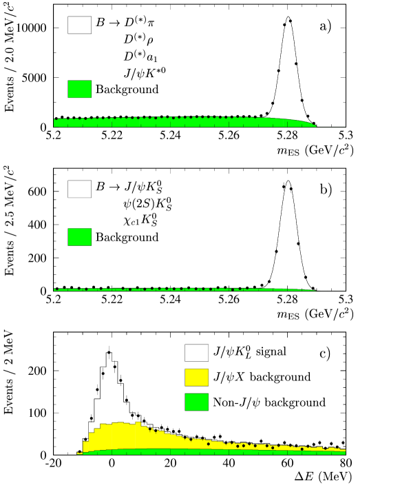
Figure 1: Distributions for $B_{\rm flav}$ and $B_{C\!P}$ candidates before vertexing requirements: a) $m_{\rm ES}$ for $B_{\rm flav}$ states; b) $m_{\rm ES}$ for $B^{0}\rightarrow{J\mskip-3.0mu/\mskip-2.0mu\psi\mskip 2.0mu}K^{0}_{\scriptscriptstyle S},\psi{(2S)}K^{0}_{\scriptscriptstyle S},\chi_{c1}K^{0}_{\scriptscriptstyle S}$ final states; and c) $\Delta E$ for the final state $B^{0}\rightarrow{J\mskip-3.0mu/\mskip-2.0mu\psi\mskip 2.0mu}K^{0}_{\scriptscriptstyle L}$.

Using exactly the same requirements, we analyze GEANT4-simulated samples of generic $B\kern 1.79993pt\overline{\kern-1.79993ptB}{}$ and signal events to check for any biases in the procedure or extracted parameters. The Monte Carlo samples are also used to assess detector response and to estimate some background sources. The values of the physics parameters assumed in the simulations are similar to those measured in the data. We used additional samples with significantly different values to check the reliability of the analysis in other regions of the parameter space.

5 Flavor tagging

The tracks that are not part of the fully reconstructed $B$ meson are used to determine whether the $B_{\rm tag}$ was a $B^{0}$ or $\kern 1.79993pt\overline{\kern-1.79993ptB}{}^{0}$ when it decayed. This determination cannot be done perfectly. If the probability of an incorrect assignment is $w$, an asymmetry that depends on the difference between $B^{0}$ and $\kern 1.79993pt\overline{\kern-1.79993ptB}{}^{0}$ tags will be reduced by a factor $D=1-2w$, frequently called the dilution. A neural network combining the outputs of physics-based algorithms is used to take into account the correlations between the different sources of flavor information and to assign the event to one of five mutually exclusive tagging categories. The dilution for each category is determined from data. Grouping tags into several categories, each with a relatively narrow range in mistag probability, increases the overall power of the tagging.

We group together events of similar character to make it possible to study systematic effects. Events with an identified primary electron or muon and a supporting kaon, if present, are assigned to the Lepton category. The KaonI category contains events with an identified kaon and a soft-pion candidate with opposite charges and similar flight direction. Soft pions from $D^{*+}$ decays are selected on the basis of their momentum and direction with respect to the thrust axis of $B_{\rm tag}$. Events with only an identified kaon are assigned to the KaonI or KaonII category depending on the estimated mistag probability. Events with only a soft-pion candidate are assigned to the KaonII category as well. The remaining events are assigned to the Inclusive or UnTagged category based on the estimated mistag probability. The UnTagged tagging category has a mistag rate near 50%, and therefore does not provide tagging information but it increases the sensitivity to the lifetime difference and allows the determination from the data of the detector charge asymmetries, as described in Sec. 7. The tagging efficiencies $t^{\alpha}$, defined after vertexing cuts, for the five categories are measured from the data and summarized in Table 4 of Sec. 8. This tagging algorithm is identical to that used in Ref. [14].

The mistag probabilities appear separately for $B^{0}$ and $\kern 1.79993pt\overline{\kern-1.79993ptB}{}^{0}$ tags in each tagging category. If we define $w^{\alpha}=(w^{\alpha}_{B^{0}}+w^{\alpha}_{\kern 1.25995pt\overline{\kern-1.25995ptB}{}^{0}})/2$ and $\Delta w^{\alpha}=w^{\alpha}_{B^{0}}-w^{\alpha}_{\kern 1.25995pt\overline{\kern-1.25995ptB}{}^{0}}$, we have that

$$w^{\alpha}_{B^{0}{\kern-1.12003pt\kern 1.25995pt\overline{\kern-1.25995ptB}{}^{0}}}=w^{\alpha}\pm\Delta w^{\alpha}/2~{}.$$ (26)

A correlation between the mistag rate and the $\Delta t$ uncertainty estimated event-by-event (discussed in Sec. 6) is observed in the Monte Carlo simulation for kaon based tags [2, 18]. For a ${\rm\Delta}t$ uncertainty less than 1.4 ${\rm\,ps}$, this correlation is found to be approximately linear:

$$w^{\alpha}=w^{\alpha}_{0}+w^{\alpha}_{\rm slope}\sigma_{\Delta t}~{}.$$ (27)

All signal mistag parameters, $w^{\alpha}_{0}$, $w^{\alpha}_{\rm slope}$ and $\Delta w^{\alpha}$, are floated in the global fit (11 in total since $w^{\tt Lepton}_{\rm slope}$ is assumed to be zero), and their results can be found in Table 4 in Sec. 8.

6 Decay time measurement and $\Delta t$ resolution function

The time interval $\Delta t=t_{\rm rec}-t_{\rm tag}$ between the two $B$ decays is calculated from the measured separation ${\rm\Delta}z$ between the decay vertex of the reconstructed $B_{\rm rec}$ meson and the vertex of the $B_{\rm tag}$ meson along the $z$-axis, using the known boost of the $\mathchar 28935\relax{(4S)}$ resonance in the laboratory, $\beta\gamma=0.56$. The method is the same as described in Sec. V in Ref. [18].

An estimated error $\sigma_{\Delta t}$ on $\Delta t$  is calculated for each event. This error accounts for uncertainties in the track parameters from the SVT and DCH hit resolution and multiple scattering, our knowledge of the beam spot size and most of the effects from the average $B$ flight length in the vertical direction as well as the ${\rm\Delta}z$ to $\Delta t$ conversion. However, it does not account for errors due to mistakes of the pattern recognition system, wrong associations of tracks to vertices, misalignment within and between the tracking devices, inaccuracies in the modeling of the amount of material in the tracking detectors and in our knowledge of the beam spot position and size, and the absolute $z$ scale. We use parameters in the $\Delta t$ resolution function, extracted from the data in the global fit (Table 5 in Sec. 8), to absorb most of these effects. Remaining systematic uncertainties are discussed in detail in Sec. 10.

We use only those events in which the vertices of the $B_{\rm rec}$ and $B_{\rm tag}$ are successfully reconstructed and for which $|\Delta t|<20$ ps and the $\Delta t$ uncertainty ($\sigma_{\Delta t}$) is less than 1.4 ps, as used in Ref. [1]. The fraction of events in data satisfying these requirements is about 85%. From Monte Carlo simulation we find that the reconstruction efficiency does not depend on the true value of $\Delta t$. Excluding 0.3% of the events that are poorly measured, the rms vertex resolution is about 160$\,\mu\rm m$ (1.0 ps). Because this resolution is poorer than that for the completely reconstructed vertex, the overall ${\rm\Delta}z$ resolution is dominated by the resolution of the $B_{\rm tag}$ vertex.

To model the $\Delta t$ resolution we use the sum of three Gaussian distributions (called core, tail and outlier components) with different means and widths:

$${\cal R}(\delta t,\sigma_{\Delta t};\vec{q}) = (1-f_{\rm tail}-f_{\rm out})h_{\rm G}(\delta t;\delta_{\rm core}\sigma_{\Delta t},S_{\rm core}\sigma_{\Delta t})+$$ (28)

$$f_{\rm tail}h_{\rm G}(\delta t;\delta_{\rm tail}\sigma_{\Delta t},S_{\rm tail}\sigma_{\Delta t})+$$

$$f_{\rm out}h_{\rm G}(\delta t;\delta_{\rm out},\sigma_{\rm out})$$

with

$$h_{\rm G}(\delta t;\delta,\sigma) = \frac{1}{\sqrt{2\pi}\sigma}\exp(-(\delta t-\delta)^{2}/(2\sigma^{2}))~{},$$ (29)

where $\vec{q}$ represents the collection of parameters needed to describe the Gaussians and $\delta t=\Delta t-\Delta t_{\rm true}$ represents the reconstruction error. The vertex reconstruction provides an event-by-event estimate for $|\delta t|$, namely $\sigma_{\Delta t}$. We incorporate the last Gaussian in Eq. (28) without reference to $\sigma_{\Delta t}$ since the outlier component is not expected to be well described by the estimated error. The first two Gaussian components allow two independent scale factors, $S_{\rm core}$ and $S_{\rm tail}$, to accommodate an overall underestimate ($>1$) or overestimate ($<1$) of the estimated errors. The core and tail Gaussian distributions are allowed to have non-zero means ($\delta_{\rm core}$ and $\delta_{\rm tail}$, respectively) to account for residual biases due to daughters of long-lived charm particles included in the $B_{\rm tag}$ vertex. Separate means are used for the core distribution of each tagging category. These means are scaled by $\sigma_{\Delta t}$ to account for a correlation observed in Monte Carlo simulation between the mean of the $\delta t$ distribution and $\sigma_{\Delta t}$ [2, 18]. This correlation is found to be approximately linear for a $\sigma_{\Delta t}$ less than 1.4 ps. The non-zero means of the resolution functions introduce an asymmetry into the otherwise symmetric $\Delta t$ distributions. The outlier Gaussian has a global width ($\sigma_{\rm out}$) and offset ($\delta_{\rm out}$), and it accounts for less than 0.3% of the reconstructed vertices. The parameters $f_{\rm tail}$ and $f_{\rm out}$ in Eq. (28) represent, respectively, the fractions of the tail and the outlier Gaussian components. In simulated events, we find no significant differences between the $\Delta t$ resolution function of the $B_{\rm flav}$, $B_{{C\!P}K^{0}_{\scriptscriptstyle S}}$ and $B_{{C\!P}K^{0}_{\scriptscriptstyle L}}$ samples. This is expected, since the $B_{\rm tag}$ vertex precision dominates the ${\rm\Delta}t$ resolution. Hence, the same resolution function is used for all modes. Residual differences are taken into account in the evaluation of systematic errors, as described in Sec. 10.

We find that the three parameters describing the outlier Gaussian component are largely correlated among themselves and with other resolution function parameters. Therefore, we fix the outlier bias $\delta_{\rm out}$ and width $\sigma_{\rm out}$ to 0 and 8 ps, respectively, and vary them in a wide range to evaluate systematic uncertainties. The resulting signal resolution function is described by a total of 12 parameters,

$$\vec{q}=\left\{S_{\rm core},\delta_{\rm core}^{\tt Lepton},\delta_{\rm core}^{\tt KaonI},\delta_{\rm core}^{\tt KaonII},\delta_{\rm core}^{\tt Inclusive},\delta_{\rm core}^{\tt UnTagged},f_{\rm tail},\delta_{\rm tail},S_{\rm tail},f_{\rm out},\delta_{\rm out},\sigma_{\rm out}\right\},$$

10 of which are floated in the final fit. Their final values can be found in Table 5 in Sec. 8.

As a cross-check, we use an alternative resolution function that is the sum of a single Gaussian distribution (centered at zero), the same Gaussian convolved with a one-sided exponential to describe the core and tail parts of the resolution function, and a single Gaussian distribution to describe the outlier component [2]. The exponential component is used to accommodate the bias due to tracks from charm decays on the $B_{\rm tag}$ side. The exponential constant is scaled by $\sigma_{\Delta t}$ to account for the previously described correlation between the mean of the $\delta t$ distribution and $\sigma_{\Delta t}$. In this case, each tagging category has a different core component fraction and exponential constant.

7 Likelihood fit method

We perform a single unbinned maximum-likelihood fit to all $B_{\rm flav}$, $B_{{C\!P}K^{0}_{\scriptscriptstyle S}}$ and $B_{{C\!P}K^{0}_{\scriptscriptstyle L}}$ events. Each event is characterized by its assigned tag category, $\alpha\in\{\tt Lepton,~{}KaonI,~{}KaonII,~{}Inclusive,$ ${\tt UnTagged\}}$; its tag-flavor type, $tag=B^{0},\kern 1.79993pt\overline{\kern-1.79993ptB}{}^{0}$ (unless it is untagged); its reconstructed event type, $rec=B^{0},\kern 1.79993pt\overline{\kern-1.79993ptB}{}^{0},{C\!P}K^{0}_{\scriptscriptstyle S},{C\!P}K^{0}_{\scriptscriptstyle L}$; the values of $\Delta t$ and $\sigma_{\Delta t}$; and a variable $\zeta$, either $m_{\rm ES}$ or $\Delta E$, used to assign the probabilities that the event is signal or background. The underlying distributions depend on whether the event is signal or any of a variety of backgrounds (together specified by $j$), on the tag category ($\alpha$), on the tag flavor ($tag$), and on the reconstructed final state type ($rec$). The contribution of a single event to the log-likelihood is

$$\ln\left[\sum_{j}{\cal F}^{\alpha,j}_{rec}(\zeta){\cal H}_{tag,rec}^{\alpha,j}(\Delta t,\sigma_{\Delta t})\right]~{}.$$ (30)

For a given reconstructed event type $rec$ and tagging category $\alpha$, ${\cal F}^{\alpha,j}_{rec}(\zeta)$ gives the probabilities that the event belongs to the signal or any of the various backgrounds indicated by $j$. Each such combination has its own PDF ${\cal H}_{tag,rec}^{\alpha,j}(\Delta t,\sigma_{\Delta t})$, which depends as well on the particular tag flavor, $tag$. This distribution is a convolution of a tagging-category-dependent time distribution, ${H}^{\alpha,j}_{tag,rec}(\Delta t_{\rm true})$, with a $\Delta t$ resolution function

$${\cal H}^{\alpha,j}_{tag,rec}(\Delta t,\sigma_{\Delta t}) = \int_{-\infty}^{+\infty}{\rm d}(\Delta t_{\rm true}){\cal R}(\Delta t-\Delta t_{\rm true},\sigma_{\Delta t};\vec{q}^{~{}\alpha,j}){H}^{\alpha,j}_{tag,rec}(\Delta t_{\rm true})$$ (31)

where

$${H}^{\alpha,j}_{tag,rec}(\Delta t_{\rm true}) = r_{rec}^{j}\left\{t^{\alpha,j}_{tag}(1-w^{\alpha,j}_{tag}){h}^{j}_{tag,rec}(\Delta t_{\rm true})\right.$$ (32)

$$\qquad+\left.t^{\alpha,j}_{{\overline{tag}}}w^{\alpha,j}_{{\overline{tag}}}{h}^{j}_{{\overline{tag}},rec}(\Delta t_{\rm true})\right\}~{}.$$

Here ${h}^{j}_{tag,rec}(\Delta t_{\rm true})$ represents the time dependence ${{\rm d}N/{\rm d}\Delta t_{\rm true}}$ described in Sec. 2, with $\Delta t_{\rm true}\equiv t$, using full expressions rather than expansions in $\Delta\Gamma$ and $z$. We indicate by $w^{\alpha,j}_{tag/{\overline{tag}}}$ the mistag fractions for category $\alpha$ and component $j$. The index ${\overline{tag}}$ denotes the opposite flavor to that given by $tag$. For events falling into tagging category UnTagged, $w^{\alpha,j}_{tag/{\overline{tag}}}=1/2$. The efficiency $t^{\alpha,j}_{tag}$ is the probability that an event whose signal/background nature is $j$ and whose true tag flavor is $tag$ will be assigned to category $\alpha$, regardless of whether the flavor assigned is correct or not. The efficiency $r^{j}_{rec}$ is the probability that an event whose signal/background nature is indicated by $j$ and whose true character is $rec$ will, in fact, be reconstructed.

7.1 PDF normalization

Every reconstructed event, whether signal or background occurs at some time $\Delta t_{\rm true}$, so

$$\int_{-\infty}^{+\infty}\,{\rm d}(\Delta t_{\rm true}){h}^{j}_{tag,rec}(\Delta t_{\rm true}) = 1~{},~{}~{}~{}{\rm for~{}all}~{}rec,tag~{}{\rm and}~{}j~{}.$$ (33)

Moreover, every event is assigned to some tag category (possibly UnTagged), thus

$$\sum_{\alpha}t^{\alpha,j}_{tag}=1~{}.$$ (34)

It follows then that the normalization of ${H}^{\alpha,j}_{tag,rec}(\Delta t_{\rm true})$ is

$$\sum_{\alpha}\sum_{tag}\int_{-\infty}^{+\infty}\,{\rm d}(\Delta t_{\rm true}){H}^{\alpha,j}_{tag,rec}(\Delta t_{\rm true})=r^{j}_{rec}~{}.$$ (35)

In this analysis the nominal normalization of ${\cal H}^{\alpha,j}_{tag,rec}(\Delta t,\sigma_{\Delta t})$ is the same as ${H}^{\alpha,j}_{tag,rec}(\Delta t_{\rm true})$ (asymptotic normalization), but fits with normalization in the interval $[-20,20]$ ps were also performed as a cross-check to evaluate possible systematic effects.

7.2 Efficiency asymmetries

For each signal or background, $j$, there is an average reconstruction efficiency, $r^{j}=(r^{j}_{B^{0}}+r^{j}_{\kern 1.25995pt\overline{\kern-1.25995ptB}{}^{0}})/2$. These average efficiencies are ultimately absorbed when we define fractions of reconstructed events falling into the different signal and background classes. In contrast, because all events fall into some tagging category (including UnTagged), the averages $t^{\alpha,j}=(t^{\alpha,j}_{B^{0}}+t^{\alpha,j}_{\kern 1.25995pt\overline{\kern-1.25995ptB}{}^{0}})/2$ are meaningful, and for $j$=signal, and $\alpha={\tt UnTagged}$ the result plays an important role. The asymmetries in the efficiencies,

$$\nu^{j} = \frac{r^{j}_{B^{0}}-r^{j}_{\kern 1.25995pt\overline{\kern-1.25995ptB}{}^{0}}}{r^{j}_{B^{0}}+r^{j}_{\kern 1.25995pt\overline{\kern-1.25995ptB}{}^{0}}}~{},$$

$$\mu^{\alpha,j} = \frac{t^{\alpha,j}_{B^{0}}-t^{\alpha,j}_{\kern 1.25995pt\overline{\kern-1.25995ptB}{}^{0}}}{t^{\alpha,j}_{B^{0}}+t^{\alpha,j}_{\kern 1.25995pt\overline{\kern-1.25995ptB}{}^{0}}}~{},$$ (36)

need to be determined because they might otherwise mimic fundamental asymmetries we seek to measure. In Appendix A we illustrate how the use of the untagged sample makes it possible to determine the asymmetries in the efficiencies. Note that asymmetries due to differences in the magnitudes of the decay amplitudes, $|A_{\rm flav}|\neq|\overline{A}_{\rm\overline{flav}}|$ and $|A_{\rm tag}|\neq|\overline{A}_{\rm\overline{tag}}|$, cannot be distinguished from the asymmetries in the efficiencies, thus are absorbed in the $\nu$, $\mu^{\alpha}$ parameters.

We fix the average tagging efficiencies $t^{\alpha,j}$ to estimates determined by counting the number of events falling into the different tagging categories, for each decay channel separately and in all the $\zeta$ range, after vertexing cuts. The parameters $\nu^{\rm sig}$ and $\mu^{\alpha,\rm sig}$ (signal events) are included as free parameters in the global fit, and are assumed to be the same for all $B^{0}$ peaking background sources. For $B^{+}$ peaking background components, the $\nu$s and $\mu$s are fixed to the values extracted from a previous unbinned maximum-likelihood fit to the tagged and untagged $\Delta t$ distributions of $B^{+}$ data used as control samples, described in Sec. 4. We neglected $\nu^{j}$ and $\mu^{\alpha,j}$ for combinatorial background sources.

7.3 Signal and background characterization

The function ${\cal F}^{\alpha,j}_{rec}(\zeta)$ in Eq. (30) describes the signal or background probability of observing a particular value of $\zeta$. It satisfies

$$\int_{\zeta_{\rm min}}^{\zeta_{\rm max}}{\rm d}\zeta\sum_{j}{\cal F}^{\alpha,j}_{rec}(\zeta)=1~{},$$ (37)

where $[\zeta_{\rm min},\zeta_{\rm max}]$ is the range of $m_{\rm ES}$/$\Delta E$ values used for analysis.

For $B_{\rm flav}$ and $B_{{C\!P}K^{0}_{\scriptscriptstyle S}}$ events, the $m_{\rm ES}$ shape is described with a single Gaussian distribution for the signal and an ARGUS parameterization for the background [18]. Based on these fits, an event-by-event signal probability $p^{\alpha,\rm sig}_{rec}(m_{\rm ES})$ can be calculated for each tagging category $\alpha$ and sample $rec$. As we do not expect signal probability differences between $B^{0}$ and $\kern 1.79993pt\overline{\kern-1.79993ptB}{}^{0}$, the $m_{\rm ES}$ fits were performed to $B_{\rm flav}^{0}$ and $\overline{B}_{\rm flav}^{0}$ events together. Due to the lack of statistics and the high purity of the sample, the $m_{\rm ES}$ fits to the $B^{0}\rightarrow\psi{(2S)}K^{0}_{\scriptscriptstyle S}$ and $B^{0}\rightarrow\chi_{c1}K^{0}_{\scriptscriptstyle S}$ samples were performed without splitting by tagging category. The component fractions ${\cal F}^{\alpha,j}_{rec}(m_{\rm ES})$ are then given by

$${\cal F}^{\alpha,\rm sig}_{rec}(m_{\rm ES}) = \left[1-f^{\alpha,\rm peak}_{rec}\right]p^{\alpha,\rm sig}_{rec}(m_{\rm ES})$$

$${\cal F}^{\alpha,\rm peak}_{rec}(m_{\rm ES}) = f^{\alpha,\rm peak}_{rec}p^{\alpha,\rm sig}_{rec}(m_{\rm ES})$$

$${\cal F}^{\alpha,\beta}_{rec}(m_{\rm ES}) = \left[1-p^{\alpha,\rm sig}_{rec}(m_{\rm ES})\right]f^{\alpha,\beta}_{rec}$$ (38)

where $\beta$ indexes the combinatorial, prompt and non-prompt, background components,

$$\sum_{\beta}f^{\alpha,\beta}_{rec}=1~{}.$$ (39)

The fraction $f^{\alpha,\rm peak}_{rec}$ of the signal Gaussian distribution is due to backgrounds that peak in the same region as the signal, determined from Monte Carlo simulation [18]. The estimated contributions are $(1.5\pm 0.6)\%$, $(0.28\pm 0.11)\%$, $(1.8\pm 0.6)\%$, $(1\pm 3)\%$ and $(3.5\pm 1.4)\%$ for the $B_{\rm flav}$, ${J\mskip-3.0mu/\mskip-2.0mu\psi\mskip 2.0mu}K^{0}_{\scriptscriptstyle S}\ (K^{0}_{\scriptscriptstyle S}\rightarrow\pi^{+}\pi^{-})$, ${J\mskip-3.0mu/\mskip-2.0mu\psi\mskip 2.0mu}K^{0}_{\scriptscriptstyle S}\ (K^{0}_{\scriptscriptstyle S}\rightarrow\pi^{0}\pi^{0})$, $\psi{(2S)}K^{0}_{\scriptscriptstyle S}$ and $\chi_{c1}K^{0}_{\scriptscriptstyle S}$ channels, respectively. A common peaking background fraction is assumed for all tagging categories within each decay mode. We take a common prompt fraction for all tagging categories for each $B_{{C\!P}K^{0}_{\scriptscriptstyle S}}$ decay channel independently. Due to the higher statistics of the $B_{\rm flav}$ sample and the significant differences in the background levels for each tagging category, $f^{\alpha,\rm prompt}_{B^{0}}=f^{\alpha,\rm prompt}_{\kern 1.25995pt\overline{\kern-1.25995ptB}{}^{0}}$ is allowed to vary with the tagging category. Note that the parameters of the ${\cal F}^{\alpha,\rm sig}_{rec}(m_{\rm ES})$ functions, determined from the set of separate unbinned maximum-likelihood fits to the $m_{\rm ES}$ distributions, are kept fixed in the global fit.

For $B_{{C\!P}K^{0}_{\scriptscriptstyle L}}$ events the background level is much higher, with significant non-combinatorial components, therefore requiring special treatment [18]. A binned likelihood fit to the $\Delta E$ spectrum in the data is used to determine the relative amounts of signal and background from $B\rightarrow{J\mskip-3.0mu/\mskip-2.0mu\psi\mskip 2.0mu}X$ events and events from a misreconstructed ${J\mskip-3.0mu/\mskip-2.0mu\psi\mskip 2.0mu}\rightarrow\ell^{+}\ell^{-}$ candidate (non-${J\mskip-3.0mu/\mskip-2.0mu\psi\mskip 2.0mu}$ background). In these fits, the signal and $B\rightarrow{J\mskip-3.0mu/\mskip-2.0mu\psi\mskip 2.0mu}X$ background distributions are obtained from inclusive ${J\mskip-3.0mu/\mskip-2.0mu\psi\mskip 2.0mu}$ Monte Carlo, while the non-${J\mskip-3.0mu/\mskip-2.0mu\psi\mskip 2.0mu}$ distribution is obtained from the ${J\mskip-3.0mu/\mskip-2.0mu\psi\mskip 2.0mu}$ dilepton mass sideband. The Monte Carlo simulation is also used to evaluate the channels that contribute to the $B\rightarrow{J\mskip-3.0mu/\mskip-2.0mu\psi\mskip 2.0mu}X$ background. Due to differences in purity and background composition, the fit is performed separately for each $K^{0}_{\scriptscriptstyle L}$ reconstruction type (EMC and IFR) and lepton type (${J\mskip-3.0mu/\mskip-2.0mu\psi\mskip 2.0mu}$ $\rightarrow$ $e^{+}e^{-}$ and ${J\mskip-3.0mu/\mskip-2.0mu\psi\mskip 2.0mu}$ $\rightarrow$ $\mu^{+}\mu^{-}$). The different inclusive ${J\mskip-3.0mu/\mskip-2.0mu\psi\mskip 2.0mu}$ backgrounds from Monte Carlo are then renormalized to the ${J\mskip-3.0mu/\mskip-2.0mu\psi\mskip 2.0mu}$ background fraction extracted from the data. The fractions are adjusted for lepton-tagged and non-lepton-tagged events in order to compensate for the observed differences in flavor tagging efficiencies in the ${J\mskip-3.0mu/\mskip-2.0mu\psi\mskip 2.0mu}$ sideband events relative to the $B_{\rm flav}$ and inclusive ${J\mskip-3.0mu/\mskip-2.0mu\psi\mskip 2.0mu}$ Monte Carlo. In addition, some of the decay modes in the inclusive ${J\mskip-3.0mu/\mskip-2.0mu\psi\mskip 2.0mu}$ background have particular $C\!P$ content. The PDF can then be formulated as

$$\sum_{j}{\cal F}_{{C\!P}K^{0}_{\scriptscriptstyle L}}^{\alpha,j}(\Delta E){\cal H}^{\alpha,j}_{tag,{C\!P}K^{0}_{\scriptscriptstyle L}}(\Delta t,\sigma_{\Delta t};\Delta E) = {\cal F}_{{C\!P}K^{0}_{\scriptscriptstyle L}}^{\alpha,\rm sig}(\Delta E){\cal H}^{\alpha,\rm sig}_{tag,{C\!P}K^{0}_{\scriptscriptstyle L}}(\Delta t,\sigma_{\Delta t})+$$

$$\sum_{j={J\mskip-3.0mu/\mskip-2.0mu\psi\mskip 2.0mu}~{}X}{\cal F}^{\alpha,j}_{{C\!P}K^{0}_{\scriptscriptstyle L}}(\Delta E){\cal H}^{\alpha,j}_{tag,{C\!P}K^{0}_{\scriptscriptstyle L}}(\Delta t,\sigma_{\Delta t})+$$

$${\cal F}^{\alpha,\rm non-{J\mskip-3.0mu/\mskip-2.0mu\psi\mskip 2.0mu}}_{{C\!P}K^{0}_{\scriptscriptstyle L}}(\Delta E)\left[\sum_{\beta}f^{\alpha,\beta}_{{C\!P}K^{0}_{\scriptscriptstyle L}}{\cal H}^{\alpha,\beta}_{tag,{C\!P}K^{0}_{\scriptscriptstyle L}}(\Delta t,\sigma_{\Delta t})\right]~{}.$$

As the ${J\mskip-3.0mu/\mskip-2.0mu\psi\mskip 2.0mu}$ lepton type is not expected to influence the $\Delta E$ shape, the PDFs are used without regard to lepton type. The $\Delta E$ PDFs are used separately for EMC and IFR $K^{0}_{\scriptscriptstyle L}$ type, and they are grouped for ${J\mskip-3.0mu/\mskip-2.0mu\psi\mskip 2.0mu}K^{0}_{\scriptscriptstyle L}$ (signal), ${J\mskip-3.0mu/\mskip-2.0mu\psi\mskip 2.0mu}K^{0}_{\scriptscriptstyle S}$ background, ${J\mskip-3.0mu/\mskip-2.0mu\psi\mskip 2.0mu}X$ background (excluding ${J\mskip-3.0mu/\mskip-2.0mu\psi\mskip 2.0mu}K^{0}_{\scriptscriptstyle S}$) and non-${J\mskip-3.0mu/\mskip-2.0mu\psi\mskip 2.0mu}$.

7.4 Signal and background structure

For signal events, a common set of mistag, $\Delta t$ resolution function, and $\nu$ and $\mu^{\alpha}$ parameters for all samples are assumed. This assumption is supported by extensive Monte Carlo studies. Peaking backgrounds originating in $B^{0}$ decays are assumed to have the same parameters as the signal. For $B^{+}$ peaking backgrounds we still assume the same resolution function as for signal, but the mistag and $\nu$, $\mu^{\alpha}$ parameters are fixed to the values extracted from the previous unbinned maximum-likelihood fit to the $B^{+}$ data. For combinatorial background components we use an empirical description of the mistags and $\Delta t$ resolution, allowing various intrinsic time dependencies. In the nominal fit we assume prompt and non-prompt components, the non-prompt component being a pure exponential dependence. As discussed in Sec. 10, fits with oscillatory, $C\!P$/$T$, $C\!PT$/$C\!P$ and $\rm DCKM$ structure have been also performed to evaluate possible systematic biases. A common set of mistags and $\Delta t$ resolution parameters, independent of the signal, is assumed for the non-${J\mskip-3.0mu/\mskip-2.0mu\psi\mskip 2.0mu}$  background in the $B_{{C\!P}K^{0}_{\scriptscriptstyle L}}$ sample and for the prompt and non-prompt background components in the $B_{\rm flav}$ and $B_{{C\!P}K^{0}_{\scriptscriptstyle S}}$ samples. In this case, the parameters $\Delta w^{\alpha}$ and $w^{\alpha}_{\rm slope}$ are fixed to zero, and the resolution model uses the core and outlier Gaussian distributions. The fraction of prompt and non-prompt component and the exponential constant of the non-prompt component in the non-${J\mskip-3.0mu/\mskip-2.0mu\psi\mskip 2.0mu}$ background are fixed to the values obtained from an external fit to the time distribution of the ${J\mskip-3.0mu/\mskip-2.0mu\psi\mskip 2.0mu}$ dilepton mass sideband. The nominal fit neglects $\nu^{j}$ and $\mu^{\alpha,j}$ for combinatorial background sources.

7.5 Free parameters for the nominal fit

The ultimate aim of the fit is to obtain simultaneously $\mathop{\rm{sgn}}({\mathop{\rm Re}}\lambda_{C\!P})\Delta\Gamma/\Gamma$, $|q/p|$, $\left({\mathop{\rm Re}}\lambda_{C\!P}/|\lambda_{C\!P}|\right){\mathop{\rm Re}}z$ and ${\mathop{\rm Im}}z$, assuming $R_{C\!P}=1$. The parameters ${\mathop{\rm Im}}\lambda_{C\!P}/|\lambda_{C\!P}|$ and $\Delta m$ are also floated to account for possible correlations and to provide an additional cross-check of the measurements, comparing our values with the BABAR $\sin{2\beta}$ result based on the same data sample [14] and recent $\Delta m$ measurements. The average $B^{0}$ lifetime, $\tau_{B}$, is fixed to the PDG value, $1.542$ ps [19]. As a cross-check we also performed fits with $R_{C\!P}$ and $\tau_{B}$ allowed to vary. All these physics parameters are by construction common to all samples and tagging categories, although the statistical power for determining each parameter comes from a particular combination of samples or $\Delta t$ dependences, as discussed in Sec. 2.

The doubly-$\rm CKM$-suppressed parameters are necessarily small and difficult to determine. In particular, ${\mathop{\rm Re}}\lambda_{\rm flav}$ occurs only multiplied by other small parameters. As a result, we have chosen to fix ${\mathop{\rm Re}}\lambda_{\rm flav}=0$. We fit for the parameter ${\mathop{\rm Im}}\lambda_{\rm flav}/|\lambda_{\rm flav}|$, but fix $|A_{\rm flav}/\overline{A}_{\rm flav}|=0.02$. We regard these two variables as formal entities, without the connection implied by taking ${\mathop{\rm Re}}\lambda_{\rm flav}=0$. We vary separately ${\mathop{\rm Im}}\overline{\lambda}_{\rm flav}/|\overline{\lambda}_{\rm flav}|$, but keep $|\overline{\lambda}_{\rm flav}|=|\lambda_{\rm flav}||p/q|^{2}$. Thus there are two free parameters, plus one fixed magnitude. We treat the tagging $\rm DCKM$ similarly. We assign a systematic error by varying the magnitudes by 100% and scanning all possible combinations of the phases (Sec. 10). This strategy provides, for the current data sample size, the optimal trade-off for all measured parameters between statistical and systematic uncertainties originating in the ambiguities of doubly-$\rm CKM$ suppression in the $B_{\rm tag}$, and to a lesser extent the $B_{\rm flav}$.

The total number of parameters that are free in the fit is 58, of which 36 parameterize the signal: physics parameters (4), cross-check physics parameters (2), single effective imaginary parts of the doubly-$\rm CKM$-suppressed phases (4), resolution function (10), mistags (11) and differences in the fraction of $B^{0}$ and $\kern 1.79993pt\overline{\kern-1.79993ptB}{}^{0}$ mesons that are tagged and reconstructed (5). The $\Delta t$ distributions, the asymmetries and the physics parameters $\mathop{\rm{sgn}}({\mathop{\rm Re}}\lambda_{C\!P})\Delta\Gamma/\Gamma$, $|q/p|$, $\left({\mathop{\rm Re}}\lambda_{C\!P}/|\lambda_{C\!P}|\right){\mathop{\rm Re}}z$, ${\mathop{\rm Im}}z$ and the cross-check parameter ${\mathop{\rm Im}}\lambda_{C\!P}/|\lambda_{C\!P}|$ were kept hidden until the analysis was finished. However, the parameter $\Delta m$, the residual $\Delta t$ distributions and asymmetries, the statistical errors and changes in the physics parameters due to changes in the analysis were not hidden.

8 Analysis results

We extract the parameters $\mathop{\rm{sgn}}({\mathop{\rm Re}}\lambda_{C\!P})\Delta\Gamma/\Gamma$, $|q/p|$, $\left({\mathop{\rm Re}}\lambda_{C\!P}/|\lambda_{C\!P}|\right){\mathop{\rm Re}}z$ and ${\mathop{\rm Im}}z$, ${\mathop{\rm Im}}\lambda_{C\!P}/|\lambda_{C\!P}|$, $\Delta m$, the parameters for doubly-$\rm CKM$-suppressed decays, the signal mistag, resolution function and $\nu$, $\mu^{\alpha}$ parameters and the empirical background parameters with the likelihood function described in Sec. 7. In Table 3 we list the signal yields in each tagging category after vertexing requirements. The purities (estimated in the region $m_{\rm ES}>5.27$ ${\mathrm{\,Ge\kern-1.00006ptV\!/}c^{2}}$ for non-$B_{{C\!P}K^{0}_{\scriptscriptstyle L}}$ samples and $|\Delta E|<10$ $\mathrm{\,Me\kern-1.00006ptV}$ for $B_{{C\!P}K^{0}_{\scriptscriptstyle L}}$ events), averaged over tagging categories, are 82%, 94% and 55%, for $B_{\rm flav}$, $B_{{C\!P}K^{0}_{\scriptscriptstyle S}}$ and $B_{{C\!P}K^{0}_{\scriptscriptstyle L}}$ candidates, respectively. The fitted signal mistag and resolution function parameters are shown, respectively, in Tables 4 and 5. The values of the asymmetries in reconstruction and tagging efficiencies are summarized in Table 6. There is good agreement with the asymmetries extracted with the counting-based approach outlined in Appendix A. Note that in the counting technique the time-dependence of UnTagged events is not used, therefore decreasing significantly the statistical power of the measurement of $\Delta\Gamma/\Gamma$.

Table 3: Signal event yields, obtained from the $m_{\rm ES}$ fits for the $B_{\rm flav}$ and $B_{{C\!P}K^{0}_{\scriptscriptstyle S}}$ samples and multiplying by the signal fraction in the $|\Delta E|<10$ $\mathrm{\,Me\kern-1.00006ptV}$ interval for the $B_{{C\!P}K^{0}_{\scriptscriptstyle L}}$ sample, after vertexing requirements.

	$B_{\rm flav}$			$B_{{C\!P}K^{0}_{\scriptscriptstyle S}}$			$B_{{C\!P}K^{0}_{\scriptscriptstyle L}}$
Tag	$B^{0}$	$\kern 1.79993pt\overline{\kern-1.79993ptB}{}^{0}$	Tot	$B^{0}$	$\kern 1.79993pt\overline{\kern-1.79993ptB}{}^{0}$	Tot	$B^{0}$	$\kern 1.79993pt\overline{\kern-1.79993ptB}{}^{0}$	Tot
Lepton	1478	1419	2897	96	98	194	35	35	70
Kaon I	2665	2672	5337	154	175	329	74	65	139
Kaon II	3183	2976	6159	181	188	369	85	66	151
Inclusive	3197	3014	6211	184	172	356	78	72	150
UnTagged	10423			585			260

Table 4: Signal tagging efficiencies and mistag parameters for each tagging category $\alpha$ as extracted from the nominal maximum-likelihood fit. Uncertainties are statistical only.

Tagging category	$t^{\alpha}(\%)$	$w^{\alpha}_{0}$	$w^{\alpha}_{\rm slope}$	$\Delta w^{\alpha}$
Lepton	$9.4\pm 0.2$	$0.026\pm 0.007$	0 (fixed)	$-0.012\pm 0.012$
Kaon I	$17.2\pm 0.3$	$0.020\pm 0.020$	$0.13\pm 0.04$	$-0.027\pm 0.013$
Kaon II	$19.9\pm 0.3$	$0.159\pm 0.024$	$0.07\pm 0.04$	$-0.042\pm 0.013$
Inclusive	$19.9\pm 0.3$	$0.265\pm 0.025$	$0.07\pm 0.04$	$-0.029\pm 0.013$
UnTagged	$33.6\pm 0.6$	—	—	—

Table 5: Signal ${\rm\Delta}t$ resolution function parameters as extracted from the nominal maximum-likelihood fit. Uncertainties are statistical only.

Parameter	Fitted value	Parameter	Fitted value
$S_{\rm core}$	$1.25\pm 0.04$	$S_{\rm tail}$	$5.7\pm 0.8$
$\delta_{\rm core}^{\tt Lepton}$	$0.02\pm 0.07$	$\delta_{\rm tail}$	$-1.5\pm 0.5$
$\delta_{\rm core}^{\tt KaonI}$	$-0.27\pm 0.05$	$f_{\rm tail}$	$0.034\pm 0.010$
$\delta_{\rm core}^{\tt KaonII}$	$-0.32\pm 0.04$	$\sigma_{\rm out}$	8 ps (fixed)
$\delta_{\rm core}^{\tt Inclusive}$	$-0.30\pm 0.04$	$\delta_{\rm out}$	0 ps (fixed)
$\delta_{\rm core}^{\tt UnTagged}$	$-0.28\pm 0.03$	$f_{\rm out}$	$0.0003\pm 0.0012$

Table 6: Values of the signal $B^{0}\kern 1.79993pt\overline{\kern-1.79993ptB}{}^{0}$ differences in reconstruction ($\nu$) and tagging ($\mu^{\alpha}$) efficiencies as extracted from the nominal maximum-likelihood fit. The results are compared with those obtained with a counting-based method.

Parameter	Nominal fit	Counting-based method
$\nu$	$0.011\pm 0.008$	$0.007\pm 0.008$
$\mu^{\tt Lepton}$	$0.024\pm 0.022$	$0.029\pm 0.042$
$\mu^{\tt KaonI}$	$-0.022\pm 0.017$	$-0.022\pm 0.029$
$\mu^{\tt KaonII}$	$0.014\pm 0.016$	$0.004\pm 0.027$
$\mu^{\tt Inclusive}$	$0.014\pm 0.016$	$0.025\pm 0.027$

The values of $\mathop{\rm{sgn}}({\mathop{\rm Re}}\lambda_{C\!P})\Delta\Gamma/\Gamma$, $|q/p|$, $\left({\mathop{\rm Re}}\lambda_{C\!P}/|\lambda_{C\!P}|\right){\mathop{\rm Re}}z$ and ${\mathop{\rm Im}}z$ extracted from the fits are given in Table 7. The fitted effective doubly-$\rm CKM$-suppressed decay parameters are also indicated. All these results can be compared to those obtained when the fit was repeated assuming $C\!PT$ invariance. The significant change of the effective doubly-$\rm CKM$-suppressed decay parameters between the two fits is due to the large correlation of these parameters with the $C\!PT$ violating parameter ${\mathop{\rm Im}}z$. The fitted value of $\Delta m$ agrees with recent $B$-Factory measurements [1, 2, 3, 4], and remains unchanged between the two fits. The fit result for ${\mathop{\rm Im}}\lambda_{C\!P}/|\lambda_{C\!P}|$ when we assume $C\!PT$  invariance agrees with our $\sin{2\beta}$ measurement based on the same data set [14]. When we allow for $C\!PT$ violation, ${\mathop{\rm Im}}\lambda_{C\!P}/|\lambda_{C\!P}|$ increases by $+0.012$ with unchanged statistical errors. The statistical correlation coefficients among all physics and cross-check physics parameters are shown in Table 8. Table 9 shows the top five statistical correlations of the physics parameters with any other free parameter in the global fit.

Table 7: Physics parameters results, from the global nominal fit and when we assume $C\!PT$ invariance. The free single effective doubly-$\rm CKM$-suppressed decay parameters are also indicated. Errors are statistical only.

Parameter	Nominal fit results	Fit results assuming $C\!PT$ invariance
$\mathop{\rm{sgn}}({\mathop{\rm Re}}\lambda_{C\!P})\Delta\Gamma/\Gamma$	$-0.008\pm 0.037$	$-0.009\pm 0.037$
$|q/p|$	$1.029\pm 0.013$	$1.029\pm 0.013$
$\left({\mathop{\rm Re}}\lambda_{C\!P}/|\lambda_{C\!P}|\right){\mathop{\rm Re}}z$	$0.014\pm 0.035$	$-$
${\mathop{\rm Im}}z$	$0.038\pm 0.029$	$-$
${\mathop{\rm Im}}\lambda_{\rm tag}/|\lambda_{\rm tag}|$	$1.5\pm 1.2$	$0.5\pm 1.0$
${\mathop{\rm Im}}\overline{\lambda}_{\rm tag}/|\overline{\lambda}_{\rm tag}|$	$-0.1\pm 1.2$	$0.8\pm 1.0$
${\mathop{\rm Im}}\lambda_{\rm flav}/|\lambda_{\rm flav}|$	$2.3\pm 1.1$	$1.4\pm 0.9$
${\mathop{\rm Im}}\overline{\lambda}_{\rm flav}/|\overline{\lambda}_{\rm flav}|$	$-0.6\pm 1.1$	$0.1\pm 0.9$

Table 8: Correlation among all the physics parameters as extracted from the simultaneous maximum-likelihood fit to the $B_{\rm flav}$ and $B_{C\!P}$ samples.

	$\mathop{\rm{sgn}}({\mathop{\rm Re}}\lambda_{C\!P})\Delta\Gamma/\Gamma$	$|q/p|$	${\mathop{\rm Im}}\lambda_{C\!P}/|\lambda_{C\!P}|$	$\left({\mathop{\rm Re}}\lambda_{C\!P}/|\lambda_{C\!P}|\right){\mathop{\rm Re}}z$	${\mathop{\rm Im}}z$
$\Delta m$	$-1.3\%$	$-2.8\%$	$-5.6\%$	$7.0\%$	$-0.2\%$
$\mathop{\rm{sgn}}({\mathop{\rm Re}}\lambda_{C\!P})\Delta\Gamma/\Gamma$		$11.0\%$	$0.4\%$	$-7.9\%$	$-1.8\%$
$|q/p|$			$-1.0\%$	$-2.4\%$	$-1.1\%$
${\mathop{\rm Im}}\lambda_{C\!P}/|\lambda_{C\!P}|$				$-10.9\%$	$17.4\%$
$\left({\mathop{\rm Re}}\lambda_{C\!P}/|\lambda_{C\!P}|\right){\mathop{\rm Re}}z$					$-3.4\%$

Table 9: Top five correlations of the physics parameters with any other free parameter of the global maximum-likelihood fit.

Physics parameter	Parameter	Correlation (%)
$\Delta m$	$S_{\rm tail}$	$-15.4$
	$\left({\mathop{\rm Re}}\lambda_{C\!P}/|\lambda_{C\!P}|\right){\mathop{\rm Re}}z$	$-5.8$
	$w^{\tt KaonI}_{0}$	$-5.8$
	$w^{\tt KaonII}_{\rm slope}$	$-4.7$
	$\delta_{\rm core}^{\tt UnTagged}$	$4.2$
$\mathop{\rm{sgn}}({\mathop{\rm Re}}\lambda_{C\!P})\Delta\Gamma/\Gamma$	$|q/p|$	$11.0$
	$\left({\mathop{\rm Re}}\lambda_{C\!P}/|\lambda_{C\!P}|\right){\mathop{\rm Re}}z$	$-7.9$
	$\nu$	$6.8$
	$\Delta w^{\tt KaonI}$	$-3.8$
	$\Delta w^{\tt KaonI}$	$-3.4$
$|q/p|$	$\nu$	$65.1$
	$\Delta w^{\tt KaonII}$	$-22.5$
	$\Delta w^{\tt KaonI}$	$-22.4$
	$\Delta w^{\tt Inclusive}$	$-15.5$
	$\mu^{{\tt KaonII}}$	$3.2$
${\mathop{\rm Im}}\lambda_{C\!P}/|\lambda_{C\!P}|$	${\mathop{\rm Im}}z$	$17.4$
	${\mathop{\rm Im}}\lambda_{\rm tag}/|\lambda_{\rm tag}|$	$14.4$
	${\mathop{\rm Im}}\overline{\lambda}_{\rm flav}/|\overline{\lambda}_{\rm flav}|$	$-6.2$
	${\mathop{\rm Im}}\overline{\lambda}_{\rm tag}/|\overline{\lambda}_{\rm tag}|$	$-5.5$
	$w^{\tt KaonII}_{0}$	$4.5$
$\left({\mathop{\rm Re}}\lambda_{C\!P}/|\lambda_{C\!P}|\right){\mathop{\rm Re}}z$	${\mathop{\rm Im}}\lambda_{C\!P}/|\lambda_{C\!P}|$	$-10.9$
	${\mathop{\rm Im}}z$	$-3.4$
	$\mu^{{\tt Lepton}}$	$2.2$
	${\mathop{\rm Im}}\lambda_{\rm tag}/|\lambda_{\rm tag}|$	$-2.0$
	$w^{\tt KaonII}_{0}$	$-1.6$
${\mathop{\rm Im}}z$	${\mathop{\rm Im}}\lambda_{\rm tag}/|\lambda_{\rm tag}|$	$61.6$
	${\mathop{\rm Im}}\overline{\lambda}_{\rm tag}/|\overline{\lambda}_{\rm tag}|$	$-56.6$
	$\Delta w^{\tt KaonI}$	$-8.0$
	$\Delta w^{\tt KaonII}$	$-6.1$
	$\Delta w^{\tt Inclusive}$	$-3.5$

Figures 2 and 3 show the $\Delta t$ distributions of the signal candidates ($m_{\rm ES}>5.27$ ${\mathrm{\,Ge\kern-1.00006ptV\!/}c^{2}}$ for $B_{\rm flav}$ and $B_{{C\!P}K^{0}_{\scriptscriptstyle S}}$ and $|\Delta E|<10$ $\mathrm{\,Me\kern-1.00006ptV}$ for $B_{{C\!P}K^{0}_{\scriptscriptstyle L}}$ samples). The points correspond to data. The curves correspond to the projections of the nominal likelihood fit weighted by the appropriate relative amounts of signal and background. The background contribution is indicated with the shaded area.

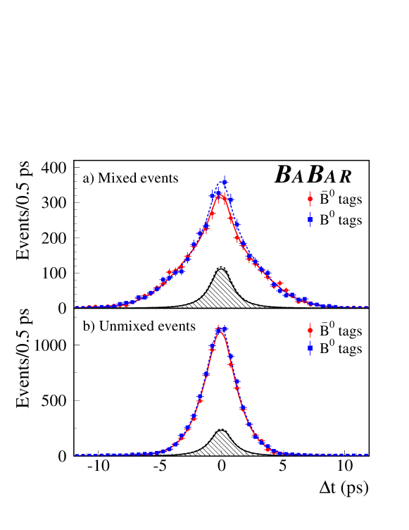
Figure 2: The $\Delta t$ distributions for (a) $B_{\rm flav}$ mixed and (b) $B_{\rm flav}$ unmixed events with a $B^{0}$ tag and with a $\kern 1.79993pt\overline{\kern-1.79993ptB}{}^{0}$ tag in the signal region, $m_{\rm ES}>5.27$ ${\mathrm{\,Ge\kern-1.00006ptV\!/}c^{2}}$. The solid (dashed) curves represent the fit projection in $\Delta t$ based on the individual signal probabilities and event-by-event $\Delta t$ uncertainty for $\kern 1.79993pt\overline{\kern-1.79993ptB}{}^{0}$ ($B^{0}$) tags. The shaded area shows the background contribution to the distributions.

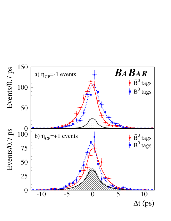
Figure 3: The $\Delta t$ distributions for (a) $B_{{C\!P}K^{0}_{\scriptscriptstyle S}}$ and (b) $B_{{C\!P}K^{0}_{\scriptscriptstyle L}}$ events with a $B^{0}$ tag and with a $\kern 1.79993pt\overline{\kern-1.79993ptB}{}^{0}$ tag in the signal region, $m_{\rm ES}>5.27$ ${\mathrm{\,Ge\kern-1.00006ptV\!/}c^{2}}$ for $B_{{C\!P}K^{0}_{\scriptscriptstyle S}}$ candidates and $|\Delta E|<10$ $\mathrm{\,Me\kern-1.00006ptV}$ for $B_{{C\!P}K^{0}_{\scriptscriptstyle L}}$ events. The solid (dashed) curves represent the fit projection in $\Delta t$ based on the individual signal probabilities and event-by-event $\Delta t$ uncertainty for $\kern 1.79993pt\overline{\kern-1.79993ptB}{}^{0}$ ($B^{0}$) tags. The shaded area shows the background contribution to the distributions.

9 Cross-checks and validation studies

We have used data and Monte Carlo samples to perform validation studies of the analysis technique. Monte Carlo tests include studies with parameterized fast Monte Carlo as well as full GEANT4 [17] simulation samples. Checks with data were performed with control samples where no $\Delta\Gamma$, $C\!P$/$T$ or $C\!PT$/$C\!P$ effects are expected. Other checks were made by analyzing the actual data sample, but using alternative tagging, vertexing and fitting configurations.

9.1 Monte Carlo simulation studies

An extensive test of the fitting procedure was performed with fast parameterized Monte Carlo simulations, generating 300 experiments with a sample size and composition corresponding to that of the data. The mistag rates and $\Delta t$ distributions were generated according to the model used in the likelihood function. The nominal fit was then performed on each of these experiments. Each experiment used the set of $m_{\rm ES}$($\Delta E$) and $\sigma_{\Delta t}$ values observed in the non-$K^{0}_{\scriptscriptstyle L}$ ($K^{0}_{\scriptscriptstyle L}$) sample. The rms spread of the residual distributions for all physics parameters (where the residual is defined as the difference between the fitted and generated values), was found to be consistent, within 10%, with the mean (Gaussian) statistical errors reported by the fits. Moreover, from these experiments it was verified that the asymmetric 68% and 90% confidence intervals provide the correct coverage. The mean values of the residual distributions were in all cases consistent with no measurement bias. A systematic error due to the precision of this study was assigned to each physics parameter. The statistical errors on all the physics parameters (Table 7) and the calculated correlation coefficients among them (Tables 8 and 9) extracted from the nominal fit to the data were consistent with the range of values obtained from these experiments: We found that 24% of the fits result in a value of the negative log-likelihood that is less (better) than that found in data.

In addition, large samples of signal and background Monte Carlo events generated with a full detector simulation were used to validate the measurement. The largest samples were generated with zero values of $\Delta\Gamma/\Gamma$, $|q/p|-1$ and $z$, but additional samples were also produced with relatively large values of these parameters. Other values (including those measured in the data) were generated with reweighting techniques. The signal Monte Carlo samples were split into samples comparable to the actual data set, keeping the relative sizes of signal $B_{\rm flav}$, $B_{{C\!P}K^{0}_{\scriptscriptstyle S}}$ and $B_{{C\!P}K^{0}_{\scriptscriptstyle L}}$ samples as observed. To check whether the selection criteria, or the analysis and fitting procedure, introduced any bias in the measurements, the nominal fit (signal only) was then applied to these experiments. The small combinatorial background in these signal samples was rejected, using only events in the signal region. Fits to the pure signal physics model, using the true $\Delta t$ distribution and true tagging information, were also performed. The means of the residual distributions from all these experiments for all the physics parameters are consistent with zero, confirming that there is no measurement bias. The rms spreads are consistent with the average reported errors and with the estimated errors in the fit to data. A systematic error is assigned to each physics parameter due to the limited Monte Carlo statistics from this test. The effect of backgrounds has been evaluated by adding an appropriate fraction of background events to the signal Monte Carlo sample and performing the fit. The $B_{C\!P}$ background samples were obtained either from simulated $B\rightarrow{J\mskip-3.0mu/\mskip-2.0mu\psi\mskip 2.0mu}X$ events or $\Delta E$ sidebands in data, while the $B_{\rm flav}$ backgrounds were obtained from generic $B\kern 1.79993pt\overline{\kern-1.79993ptB}{}$ Monte Carlo. We find no evidence of bias in any of the physics parameters.

9.2 Cross-checks with data

We fit subsamples selected by choosing a tagging category and running period. Fits using only the $B^{0}\rightarrow D^{(*)-}X^{+}$ or $B^{0}\rightarrow{J\mskip-3.0mu/\mskip-2.0mu\psi\mskip 2.0mu}K^{*0}(K^{+}\pi^{-})$ specific channels for $B_{\rm flav}$, and $B_{{C\!P}K^{0}_{\scriptscriptstyle S}}$ or $B_{{C\!P}K^{0}_{\scriptscriptstyle L}}$ only for $B_{C\!P}$, were also performed. We found no statistically significant differences in the results for the different subsets. We also varied the maximum values of $|\Delta t|$ and $\sigma_{\Delta t}$ accepted between 5 and 30 ps, and 0.6 and 2.2 ps, respectively. Again, we did not find statistically significant changes in the fitted values of the physics parameters.

In order to verify that the results are stable under variation of the vertexing algorithm that is used in the measurement of $\Delta t$, we used alternative (less powerful) methods [18]. In order to reduce statistical fluctuations due to different events being selected, the comparison between the alternative and nominal methods was performed using only the common events. Observed variations were consistent with anticipated statistical fluctuations and with the systematic error assigned to the resolution function (see Sec. 10).

The stability of the results under variation of the tagging algorithm was studied by repeating the fit using the tagging algorithm used in Ref. [18]. The algorithm used in that analysis had an effective tagging efficiency, $Q=\sum_{\alpha}t^{\alpha}\left(1-2w^{\alpha}\right)^{2}$, about 7% lower than the one used here. The variation observed in the physics parameters is consistent with the statistical differences.

The average $B^{0}$ lifetime was fixed in the nominal fit to the PDG value [19]. This value was obtained by averaging measurements based on flavor eigenstate samples and assuming negligible effects from $\Delta\Gamma/\Gamma$, $|q/p|$ and $C\!PT$ violation. Measurements that do not use tagged events are not affected by $|q/p|$ and $C\!PT$ violation, but are by a non-zero value $\Delta\Gamma/\Gamma$ at second order, as discussed in Sec. 2. Therefore we do not expect significant effects from the fixed average $B^{0}$ lifetime. However, to check the consistency of the result, the fit was repeated with $\tau_{B}$ left free. The resulting $\tau_{B}$ was about two standard deviations below the nominal value assumed in our analysis, before bias corrections and taking into account the statistical error from the fit and the present $\tau_{B}$ uncertainty. The changes of the physics parameters were within statistical errors. Nevertheless, a systematic error was assigned using the variation of each physics parameter repeating the fit with $\tau_{B}$ fixed after a change of two standard deviations of the present uncertainty ($\pm 0.032$ ps).

Similarly, fits with $R_{C\!P}$ floated were performed. The resulting $R_{C\!P}$ value was consistent with 1 (the fixed nominal value), within one standard deviation (statistical only). The changes observed in the physics parameters were consistent with their statistical uncertainties. Systematic errors due to fixing $R_{C\!P}$ at unity were set by changing $R_{C\!P}$ by twice the statistical uncertainty determined by floating it ($\pm 10\%$). The resulting variation in each parameter was taken as the systematic error.

The robustness of the fit was also tested by modifying the nominal PDF normalization, as described by Eq. (33), so that the analysis was insensitive to the relative amount of $B^{0}$ and $\kern 1.79993pt\overline{\kern-1.79993ptB}{}^{0}$  tagged events. As a consequence, the statistical power of $|q/p|$ was dramatically reduced, since the sensitivity of this parameter comes largely from the differences in time-integrated $B^{0}$ and $\kern 1.79993pt\overline{\kern-1.79993ptB}{}^{0}$ rates. In addition, the fit was also performed assuming an independent set of resolution function parameters for each tagging category. In all cases the results are compatible within statistical differences with the nominal fit results. Finally, the tagging efficiencies $t^{\alpha,j}$ were alternatively determined from the $B_{\rm flav}$ sample and assumed to be the same for all samples (rather than to use the estimate from each sample separately, as in the nominal fit). The change in the values of the physics parameters was found to be negligible.

Control samples in data from $B^{+}$ decays (treated in a fashion analogous to that described in Sec. 4) have also been used to validate the analysis technique, since in these samples we expect zero values for $\Delta\Gamma/\Gamma$, $|q/p|$ and $z$. For the $B_{\rm flav}$ sample we used the $B^{+}\rightarrow\overline{D}^{(*)0}\pi^{+}$ decay channel, and for the $B_{C\!P}$ sample the charmonium $B^{+}$ decays. Due to the absence of mixing and $C\!P$ violation in these samples, the check was performed fixing $\Delta m=0$ and $|q/p|=1$ in the $B_{\rm flav}$ sample, and $\Delta m=0.489$ ps^-1 and ${\mathop{\rm Im}}\lambda_{C\!P}/|\lambda_{C\!P}|=0$ in the $B_{C\!P}$ sample, fitting only for $\mathop{\rm{sgn}}({\mathop{\rm Re}}\lambda_{C\!P})\Delta\Gamma/\Gamma$, $\left({\mathop{\rm Re}}\lambda_{C\!P}/|\lambda_{C\!P}|\right){\mathop{\rm Re}}z$ and ${\mathop{\rm Im}}z$. No statistically significant deviations from zero were observed.

10 Systematic uncertainties

We estimate systematic uncertainties with studies performed on both data and Monte Carlo simulation samples. A summary of the non-negligible sources and results is shown in Table 10. In the following, the individual contributions are referenced by the lettered lines in this table.

Table 10: Summary of systematic uncertainties on the measurement of $\mathop{\rm{sgn}}({\mathop{\rm Re}}\lambda_{C\!P})\Delta\Gamma/\Gamma$, $|q/p|$, $\left({\mathop{\rm Re}}\lambda_{C\!P}/|\lambda_{C\!P}|\right){\mathop{\rm Re}}z$ and ${\mathop{\rm Im}}z$.

Systematics source	$\mathop{\rm{sgn}}({\mathop{\rm Re}}\lambda_{C\!P})\Delta\Gamma/\Gamma$	$|q/p|$	$\left({\mathop{\rm Re}}\lambda_{C\!P}/|\lambda_{C\!P}|\right){\mathop{\rm Re}}z$	${\mathop{\rm Im}}z$
Likelihood fit procedure
(a) Parameterized MC test	$0.003$	$0.001$	$0.003$	$0.003$
(b) GEANT4 MC test	$0.005$	$0.007$	$0.004$	$0.016$
$\Delta t$ resolution function
(c) Res. funct. parameterization	$0.007$	$0.001$	$0.008$	$0.003$
(d) $z$ scale and boost	$0.003$	$0.001$	$0.002$	$<0.001$
(e) Beam spot	$0.008$	$0.002$	$0.001$	$0.011$
(f) SVT alignment	$0.006$	$0.001$	$0.001$	$0.011$
(g) Outliers	$0.002$	$<0.001$	$<0.001$	$<0.001$
Signal properties
(h) Average $B^{0}$ lifetime	$0.004$	$0.001$	$0.004$	$<0.001$
(i) Direct $C\!P$ violation	$0.002$	$0.004$	$0.001$	$0.003$
(j) Doubly-$\rm CKM$-suppressed decays	$0.008$	$0.004$	$0.032$	$0.006$
(k) Residual charge asymmetries	$0.005$	$0.006$	$0.004$	$0.006$
Background properties and structure
(l) Signal probability	$0.002$	$0.001$	$0.002$	$0.001$
(m) Fraction of peaking background	$<0.001$	$<0.001$	$0.004$	$<0.001$
(n) $\Delta t$ structure	$0.002$	$0.001$	$0.001$	$0.001$
(o) $\Delta\Gamma$/$C\!PT$/$C\!P$/$T$/Mixing/$\rm DCKM$	$0.001$	$0.002$	$0.002$	$<0.001$
(p) Residual charge asymmetry	$<0.001$	$0.001$	$<0.001$	$<0.001$
(q) $K^{0}_{\scriptscriptstyle L}$ specific systematics	$0.004$	$<0.001$	$0.004$	$0.003$
Total systematics	0.018	0.011	0.034	0.025

10.1 Likelihood fit procedure

Several sources of systematics due to the likelihood fit procedure are considered. We first include the results from the tests performed using the fast parameterized Monte Carlo (a) and the full GEANT4 signal Monte Carlo events (b), as described in Sec. 9.1. We take the larger of the observed bias (mean of the residual distributions) and its statistical error as the systematic error. No corrections are applied to the central values extracted from the fit to the data since no statistically significant bias is observed. Note that the GEANT4 simulation addresses the underlying assumption that the fit properly accounts for residual differences in the mistag, resolution function, $\nu$, $\mu^{\alpha}$ parameters for $B_{\rm flav}$, $B_{{C\!P}K^{0}_{\scriptscriptstyle S}}$ and $B_{{C\!P}K^{0}_{\scriptscriptstyle L}}$ samples and differences in $\Delta t$ resolution for correct and wrong tags [18].

We also consider the impact on the measured physics parameters of the asymptotic PDF normalization. The effect is evaluated by varying the fitted values using a normalization in the range defined by the $\Delta t$ cut. Finally, the fixed tagging efficiencies are varied within their statistical uncertainties. The two contributions are found to be negligible.

10.2 $\Delta t$ resolution function

The resolution model used in the analysis, consisting of the sum of three Gaussian distributions, is expected to be flexible enough to accommodate the actual resolution function. To assign a systematic error to the assumption of this model, we use the alternative model described in Sec. 6, with a Gaussian distribution plus the same Gaussian convolved with one exponential function, for both signal and background. The results for all physics parameters obtained from the two resolution models are consistent within statistical uncertainties. However, we assign the difference of central values as a systematic uncertainty (c).

In addition a number of parameters that are integral to the determination of $\Delta t$ are varied according to known uncertainties. The PEP-II boost, estimated from the beam energies, has an uncertainty of 0.1% [16]. The absolute $z$-scale uncertainty has been evaluated to be less than 0.4%. This estimate was obtained by measuring the beam pipe dimensions with scattered protons and comparing to optical survey data. Therefore, the boost and $z$-scale systematics are evaluated by varying by $\pm 0.6\%$ the reconstructed $\Delta t$ and $\sigma_{\Delta t}$ (d). The uncertainty on the beam spot, which is much wider than it is high, is taken into account by moving its vertical position (the direction most valuable in vertexing) by 20 and 40 $\mu$m and increasing the vertical dimension by 30 and 60 $\mu$m (e). Finally, the systematic uncertainty due to possible SVT internal misalignment is evaluated by applying a number of possible misalignment scenarios to a sample of simulated events and comparing the values of the fitted physics parameters from these samples to the case of perfect alignment (f).

Fixing the width and bias of the outlier component, respectively to 8.0 and 0.0 ps, introduces systematic errors. To estimate the uncertainty we add in quadrature the variation observed in the physics parameters when the bias changes by $\pm$5 ps, the width varies between 6 and 12 ps and the outlier distribution is assumed to be flat (g).

10.3 Signal properties

As described in Sec. 9.2, the uncertainty from fixing the average $B^{0}$ lifetime has been evaluated by moving its central value by $\pm 0.032$ ps (h), twice the current uncertainty [19]. Possible direct $C\!P$ violation in the $B_{C\!P}$ sample was taken into account by varying $R_{C\!P}$ by $\pm 10\%$ (i).

Systematics from doubly-$\rm CKM$-suppressed decays arise due to uncertainties in ${\mathop{\rm Re}}\lambda_{\rm tag}$, ${\mathop{\rm Re}}\overline{\lambda}_{\rm tag}$, ${\mathop{\rm Re}}\lambda_{\rm flav}$ and ${\mathop{\rm Re}}\overline{\lambda}_{\rm flav}$. In order to evaluate this contribution, samples of parameterized Monte Carlo tuned to the data sample, with all possible values of the doubly-$\rm CKM$-suppressed phases were generated, assuming a single hadronic decay channel contributing to the $B_{\rm tag}$ and to the $B_{\rm flav}$. The generation was made for maximal values of $|A_{\rm tag}/\overline{A}_{\rm tag}|$ and $|A_{\rm flav}/\overline{A}_{\rm flav}|$, assuming a 100% uncertainty on its estimate based on the elements of the CKM matrix, $\approx 0.02$ [19]. For the Lepton tagging category, largely dominated by semileptonic $B$ decays, we assumed $|\lambda_{\rm tag}|$ to be zero. Using the fit results from all these samples, we evaluated the larger of the offset with respect to the generated value and its statistical uncertainty, for each possible configuration of phases. The systematic error assigned was the largest value among all configurations (j). This is the dominant source of systematic uncertainty for the measurement of $\left({\mathop{\rm Re}}\lambda_{C\!P}/|\lambda_{C\!P}|\right){\mathop{\rm Re}}z$, primarily due to the $\rm DCKM$ effects in the tagging $B$ meson. Similar studies performed with more than one hadronic channel indicated the destructive interference among the different decay modes, proving that our prescription to assign the systematics assuming a single effective channel is conservative.

Charge asymmetries induced by a difference in the detector response for positive and negative tracks are included in the PDF and extracted together with the other parameters from the time-dependent analysis. Thus, they do not contribute to the systematic error, but rather are incorporated into the statistical error at a level determined by the size of the $B_{\rm flav}$ data sample. Nevertheless, in order to account for any possible and residual effect, we assigned a systematic uncertainty as follows. We reran the $B$ reconstruction, vertexing and tagging code after killing randomly and uniformly (no momentum or angular dependence) 5% of positive and negative tracks in the full Monte Carlo sample. This 5% is on average more than a factor three larger than the precision with which the parameters $\nu$ and $\mu^{\alpha}$ have been measured in the data. The half difference between the results obtained for positive and negative tracks is assigned as a systematic error (k).

10.4 Background properties and structure

The event-by-event signal probability $p^{\alpha,\rm sig}_{rec}(m_{\rm ES})$ for $B_{\rm flav}$ and $B_{{C\!P}K^{0}_{\scriptscriptstyle S}}$ samples was fixed to the values obtained from the $m_{\rm ES}$ fits. We compared the results from the nominal fits to the values obtained by changing one sigma up and down all the $m_{\rm ES}$ distribution parameters, taking into account their correlations. This was performed simultaneously for all tagging categories, and independently for the $B_{\rm flav}$ and $B_{{C\!P}K^{0}_{\scriptscriptstyle S}}$ samples. Alternatively, we also used a flat signal probability distribution: events belonging to the sideband region ($m_{\rm ES}$$<$5.27 ${\mathrm{\,Ge\kern-1.00006ptV\!/}c^{2}}$) are assigned a signal probability of zero, while we gave a signal probability equal to the purity of the corresponding sample to signal region events ($m_{\rm ES}$$>$5.27 ${\mathrm{\,Ge\kern-1.00006ptV\!/}c^{2}}$). The differences among fitted physical parameters with respect to the default method were found to be consistent within the statistical differences. We determined the systematic error due to this parameterization by varying the signal probability by the statistical error in the purity. The final systematic error was taken to be the larger of the one-sigma variations found for the two methods (l). The uncertainty on the fraction of peaking background was estimated by varying the fractions according to its uncertainty separately for the $B_{\rm flav}$ sample and each $B_{{C\!P}K^{0}_{\scriptscriptstyle S}}$ decay mode (m). The effective $\eta_{C\!P}$ of the $B_{{C\!P}K^{0}_{\scriptscriptstyle S}}$ peaking background, assumed to be zero in the nominal fit, was also varied between $+1$ and $-1$ and found to be negligible.

Another source of systematic uncertainty originates from the assumption that the $\Delta t$ structure of the combinatorial background in the $m_{\rm ES}$ sideband region is a good description of the structure in the signal region. However, the background composition changes slightly as a function of $m_{\rm ES}$, since the fraction due to continuum production slowly decreases towards the $B$ mass. To study this effect, we first varied the lower edge of the $m_{\rm ES}$ distributions from 5.20 ${\mathrm{\,Ge\kern-1.00006ptV\!/}c^{2}}$ to 5.27 ${\mathrm{\,Ge\kern-1.00006ptV\!/}c^{2}}$, simultaneously for the $B_{\rm flav}$ and $B_{{C\!P}K^{0}_{\scriptscriptstyle S}}$ samples, observing a good stability of the result. We also split the sideband region in seven equal slices each 10 ${\mathrm{\,Me\kern-1.00006ptV\!/}c^{2}}$ wide and used each of these ranges to perform a standard fit. The quadratic sum of the extrapolation to the $B$ mass region and the error on it was assigned as systematic uncertainty (n).

As described in Sec. 7, the nominal likelihood fit assumes that there is no $\Delta\Gamma$, $C\!P$/$T$, $C\!PT$/$C\!P$, mixing and doubly-$\rm CKM$-suppressed decays content in the combinatorial background components ($B_{\rm flav}$ and $B_{{C\!P}K^{0}_{\scriptscriptstyle S}}$ samples) and in the non-${J\mskip-3.0mu/\mskip-2.0mu\psi\mskip 2.0mu}$ background ($B_{{C\!P}K^{0}_{\scriptscriptstyle L}}$ sample). To evaluate the effect of this assumption we repeated the fit but now assuming non-zero values of $\Delta\Gamma$, $|q/p|$, $z$, ${\mathop{\rm Im}}\lambda_{C\!P}$ and $\Delta m$, varying $\eta_{C\!P}$ of the background by $\pm 1$. The check was performed by introducing in the PDF an independent set of physics parameters and assuming maximal mixing and $C\!P$ violation ($\Delta m$ and ${\mathop{\rm Im}}\lambda_{C\!P}/|\lambda_{C\!P}|$ fixed to 0.489 ps^-1 [19] and 0.75 [14], respectively). Doubly-$\rm CKM$-suppressed decay effects were included assuming the maximal values of $|A_{\rm tag}/\overline{A}_{\rm tag}|$, $|A_{\rm flav}/\overline{A}_{\rm flav}|$ and scanning all the possible values of the $B^{0}$ and $\kern 1.79993pt\overline{\kern-1.79993ptB}{}^{0}$ phases for $B_{\rm flav}$ and $B_{\rm tag}$. The systematic uncertainty was evaluated simultaneously for all of these sources (o).

The uncertainty due to the $B^{+}$ lifetime has been evaluated by moving the central value according to the current uncertainty [19]. It was found to be negligible. The $B^{+}$ mistags and the differences in the fraction of $B^{+}$ and $B^{-}$ mesons that are tagged and reconstructed were varied according to their statistical errors as obtained from the fit to the $B^{+}$ data. They were found also to be negligible. Uncertainties from charge asymmetries in combinatorial background components (neglected in the nominal fit) were evaluated by repeating the fit with a new set of $\nu$ and $\mu^{\alpha}$ parameters. The measured values of $\nu$ and $\mu^{\alpha}$ are found to be compatible with zero and the variation of the physical parameters with respect to the nominal fit is assigned as systematic error (p).

For the $B_{{C\!P}K^{0}_{\scriptscriptstyle L}}$ channel [18], the signal and non-${J\mskip-3.0mu/\mskip-2.0mu\psi\mskip 2.0mu}$ background fractions are varied according to their statistical uncertainties as obtained from the fit to the $\Delta E$ distribution. We also vary background parameters, including the ${J\mskip-3.0mu/\mskip-2.0mu\psi\mskip 2.0mu}X$ branching fractions, the assumed $\eta_{C\!P}$, the $\Delta E$ shape and the fraction and effective lifetime of the prompt and non-prompt non-${J\mskip-3.0mu/\mskip-2.0mu\psi\mskip 2.0mu}$ components. The differences observed between data and Monte Carlo simulation for the $K^{0}_{\scriptscriptstyle L}$ angular resolution and for the fractions of $B^{0}\rightarrow{J\mskip-3.0mu/\mskip-2.0mu\psi\mskip 2.0mu}K^{0}_{\scriptscriptstyle L}$ events reconstructed in the EMC and IFR are used to evaluate a systematic uncertainty due to the simulation of the $K^{0}_{\scriptscriptstyle L}$  reconstruction. Finally, an additional contribution is assigned to the correction applied to Lepton events due to the observed differences in flavor tagging efficiencies in the ${J\mskip-3.0mu/\mskip-2.0mu\psi\mskip 2.0mu}$ sideband relative to $B_{\rm flav}$ and inclusive ${J\mskip-3.0mu/\mskip-2.0mu\psi\mskip 2.0mu}$ Monte Carlo. Conservatively, this error was evaluated comparing the fit results with and without the correction. The total $B_{{C\!P}K^{0}_{\scriptscriptstyle L}}$ specific systematics is evaluated by taking the quadratic sum of the individual contributions (q).

10.5 Summary of systematic uncertainties

All individual systematic contributions described above and summarized in Table 10 are added in quadrature. The dominant source of systematic error in the measurement of $\left({\mathop{\rm Re}}\lambda_{C\!P}/|\lambda_{C\!P}|\right){\mathop{\rm Re}}z$ is due to our limited knowledge of the doubly-$\rm CKM$-suppressed decays, which also contributes significantly to the other measurements. The limited Monte Carlo statistics are a dominant source of systematics for $|q/p|$, ${\mathop{\rm Im}}z$ and to a lesser extent to $\mathop{\rm{sgn}}({\mathop{\rm Re}}\lambda_{C\!P})\Delta\Gamma/\Gamma$. Residual charge asymmetries also dominate the systematics on $|q/p|$. Our limited knowledge of the beam spot and SVT alignment also reflects significantly on ${\mathop{\rm Im}}z$ and $\mathop{\rm{sgn}}({\mathop{\rm Re}}\lambda_{C\!P})\Delta\Gamma/\Gamma$. The systematic error on $\mathop{\rm{sgn}}({\mathop{\rm Re}}\lambda_{C\!P})\Delta\Gamma/\Gamma$ also receives a non-negligible contribution from our understanding of the resolution function. The systematic uncertainties on $\mathop{\rm{sgn}}({\mathop{\rm Re}}\lambda_{C\!P})\Delta\Gamma/\Gamma$ and $|q/p|$ when $C\!PT$ is assumed to be a good symmetry were evaluated similarly, and found to be, respectively, $\pm 0.020$ and $\pm 0.012$.

11 Summary and discussion of results

The conventional analysis of mixing and $C\!P$ violation in the neutral $B$ meson system neglects possible contributions from several sources that are expected to be small. These include the difference of the lifetimes of the two neutral $B$ meson mass eigenstates, the $C\!P$- and $T$-violating quantity $|q/p|-1$, which is proportional to ${\mathop{\rm Im}}(\Gamma_{12}/M_{12})$, and potential $C\!PT$ violation. To measure or extract limits on these quantities requires the full expressions for time dependence in mixing and $C\!P$ violation and consideration of systematic issues that might mimic fundamental asymmetries we seek to measure, like detector charge asymmetries, different resolution function for positive and negative $\Delta t$, and doubly-$\rm CKM$-suppressed decays from both fully reconstructed final flavor states and non-leptonic tagging states.

Our analysis of approximately 31,000 fully reconstructed flavor eigenstates and 2600 $C\!P$ eigenstates sets new limits on the difference of decay widths of $B^{0}$ mesons and on the $C\!P$, $T$, and $C\!PT$ violation intrinsic to $B^{0}{\kern-1.60004pt\kern 1.79993pt\overline{\kern-1.79993ptB}{}^{0}}$ mixing. The six independent parameters governing mixing ($\Delta m$, $\Delta\Gamma/\Gamma$), $C\!PT$/$C\!P$ violation (${\mathop{\rm Re}}z$, ${\mathop{\rm Im}}z$) and $C\!P$/$T$ violation (${\mathop{\rm Im}}\lambda_{C\!P}$, $|q/p|$) are extracted from a single fit of both fully reconstructed $C\!P$ and non-$C\!P$ events, tagged and untagged. This provides the sensitivity required to separate the small effects we seek from asymmetries in detector response and from potentially obscuring correlations in the decays of the two $B$ mesons. The preliminary results are

$$\begin{array}[]{ r@{\ \ =\ }r@{.}l@{\pm 0.}l@{{\rm(stat.)}\pm 0.} l@{{\rm{(syst.)}}\ \ [}r@{,}l@{]}l}\mathop{\rm{sgn}}({\mathop{\rm Re}}\lambda_{C\!P})\Delta\Gamma/\Gamma&-0&008&037&018&-0.084&0.068&~{},\\ |q/p|&1&029&013&011&1.001&1.057&~{},\\ \left({\mathop{\rm Re}}\lambda_{C\!P}/|\lambda_{C\!P}|\right){\mathop{\rm Re}}z&0&014&035&034&-0.072&0.101&~{},\\ {\mathop{\rm Im}}z&0&038&029&025&-0.028&0.104&~{}.\end{array}$$

The values in square brackets indicate the 90% confidence-level intervals. When estimating the limits we also evaluated multiplicative contributions to the systematic error, adding in quadrature with the additive systematic uncertainties. Assuming $C\!PT$ invariance the results are

$$\begin{array}[]{ r@{\ \ =\ }r@{.}l@{\pm 0.}l@{{\rm(stat.)}\pm 0.} l@{{\rm{(syst.)}}\ \ [}r@{,}l@{]}l}\mathop{\rm{sgn}}({\mathop{\rm Re}}\lambda_{C\!P})\Delta\Gamma/\Gamma&-0&009&037&020&-0.087&0.069&~{},\\ |q/p|&1&029&013&012&1.000&1.058&~{}.\end{array}$$

The parameters $\Delta m$ and ${\mathop{\rm Im}}\lambda_{C\!P}/|\lambda_{C\!P}|$ are allowed to float, so that recent $B$-Factory $\Delta m$ results [1, 2, 3, 4] and our $\sin 2\beta$ analysis based on the same data sample [14] provide a cross-check. The value of the $C\!P$/$T$-violating parameter ${\mathop{\rm Im}}\lambda_{C\!P}/|\lambda_{C\!P}|$ increases by $+0.012$ when $C\!PT$ violation is allowed in the fit.

The results are consistent with Standard Model expectations and with $C\!PT$ invariance. To date, these are the best limits on the difference of decay widths of $B^{0}$ mesons and the strongest test of $C\!PT$ invariance outside the neutral kaon system [12]. The limit on $C\!P$ and $T$ violation in mixing is independent of and consistent with our previous measurement based on the analysis of inclusive dilepton events [20]. Fig. 4 shows the results in the $(|q/p|-1,|z|)$ plane, comparing them to the BABAR measurement of $|q/p|$ made with dileptons and to the Standard Model expectations. All the other results are also consistent with previous analyses [4, 6, 7, 13]. While the Standard Model predictions for $\Delta\Gamma$ and $|q/p|-1$ are still well below our current limits and no $C\!PT$ violation is anticipated, higher precision measurements may still bring surprises.

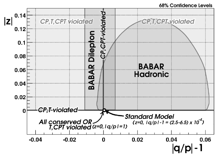
Figure 4: Favored regions at 68% confidence level in the $(|q/p|-1,|z|)$ plane determined by this analysis (”Hadronic”) and by the BABAR measurement of the dilepton asymmetry [20]. The axis labels reflect the requirements that both $C\!P$ and $T$ be violated if $|q/p|\neq 1$ and that both $C\!P$ and $C\!PT$ be violated if $|z|\neq 0$. The region shown for this analysis is constrained to lie within the physical region $|z|\geq 0$ and is chosen to exclude the maximum range of alternative hypotheses given the a priori low probability of obtaining $|z|=0$ due to phase-space considerations. The dilepton measurement constrains $|q/p|$ without assumptions on the value of $|z|$. The Standard Model expectation is obtained from Ref. [21].

12 Acknowledgments

We are grateful for the extraordinary contributions of our PEP-II colleagues in achieving the excellent luminosity and machine conditions that have made this work possible. The success of this project also relies critically on the expertise and dedication of the computing organizations that support BABAR. The collaborating institutions wish to thank SLAC for its support and the kind hospitality extended to them. This work is supported by the US Department of Energy and National Science Foundation, the Natural Sciences and Engineering Research Council (Canada), Institute of High Energy Physics (China), the Commissariat à l’Energie Atomique and Institut National de Physique Nucléaire et de Physique des Particules (France), the Bundesministerium für Bildung und Forschung and Deutsche Forschungsgemeinschaft (Germany), the Istituto Nazionale di Fisica Nucleare (Italy), the Foundation for Fundamental Research on Matter (The Netherlands), the Research Council of Norway, the Ministry of Science and Technology of the Russian Federation, and the Particle Physics and Astronomy Research Council (United Kingdom). Individuals have received support from the A. P. Sloan Foundation, the Research Corporation, and the Alexander von Humboldt Foundation.

Appendix A Efficiency asymmetries

The use of untagged data is essential to determining the asymmetries in the tagging and reconstruction efficiencies. To indicate how the various samples enter we provide a simple example using only time-integrated quantities. In practice we use a time-dependent analysis, which gives better precision because it uses more information. Suppressing the tag category $\alpha$, the signal or background component, $j$, and writing the reconstruction efficiencies as $r=r^{j}_{B^{0}},\,{\overline{r}}=r^{j}_{\kern 1.25995pt\overline{\kern-1.25995ptB}{}^{0}}$ and the tagging efficiencies as $t=t^{\alpha,j}_{B^{0}},\,{\overline{t}}=t^{\alpha,j}_{\kern 1.25995pt\overline{\kern-1.25995ptB}{}^{0}}$, Eq. (36) reads

$$\nu = \frac{r-{\overline{r}}}{r+{\overline{r}}}$$

$$\mu = \frac{t-{\overline{t}}}{t+{\overline{t}}}~{}.$$ (41)

Using the numbers of signal events that are tagged and have a reconstructed $B^{0}$ ($X$), those tagged and having a $\kern 1.79993pt\overline{\kern-1.79993ptB}{}^{0}$ ($Y$), those untagged with a reconstructed $B^{0}$ ($Z$) and finally those untagged with a reconstructed $\kern 1.79993pt\overline{\kern-1.79993ptB}{}^{0}$ ($W$) we can determine the required asymmetries [18]. To see this, note that if the total number of $B^{0}{\kern-1.60004pt\kern 1.79993pt\overline{\kern-1.79993ptB}{}^{0}}$ pairs is $N$, and neglecting $\Delta\Gamma$, $|q/p|$ and $z$ corrections, there are $N_{u}=N(1+[1/(1+x_{d}^{2})])/2$ unmixed events (i.e. $B^{0}{\kern-1.60004pt\kern 1.79993pt\overline{\kern-1.79993ptB}{}^{0}}$) and $N_{m}=N(1-[1/(1+x_{d}^{2})])/2$ mixed events (i.e. $B^{0}B^{0}$ or $\kern 1.79993pt\overline{\kern-1.79993ptB}{}^{0}\kern 1.79993pt\overline{\kern-1.79993ptB}{}^{0}$), where $x_{d}=\tau_{B}\Delta m$, so

$$X = rtN_{m}/2+r{\overline{t}}N_{u}/2$$

$$Y = {\overline{r}}{\overline{t}}N_{m}/2+{\overline{r}}tN_{u}/2$$

$$Z = r(1-t)N_{m}/2+r(1-\overline{t})N_{u}/2$$

$$W = {\overline{r}}(1-\overline{t})N_{m}/2+{\overline{r}}(1-t)N_{u}/2~{}.$$ (42)

Setting $U=X+Z$ and $V=Y+W$, we find

$$\nu=\frac{U-V}{U+V}\qquad,~{}~{}~{}~{}~{}~{}\mu=(1+x_{d}^{2})\frac{(Y/V)-(X/U)}{(Y/V)+(X/U)}~{}.$$ (43)

Corrections to these equations have to be applied due to non-zero values of $\Delta\Gamma$, $|q/p|-1$ and $z$. The use of untagged events is essential to the determination of $\nu$ and $\mu$.

References

- [1] BABAR Collaboration, B. Aubert et al., Phys. Rev. Lett. 88, 221802 (2002).
- [2] BABAR Collaboration, B. Aubert et al., hep-ex/0212017, to appear in Phys. Rev. D .
- [3] BABAR Collaboration, B. Aubert et al., Phys. Rev. Lett. 88, 221803 (2002).
- [4] Belle Collaboration, N.C. Hastings et al., hep-ex/0212033, to appear in Phys. Rev. D .
- [5] A.S. Dighe et al., Nucl. Phys. B 624, 377 (2002).
- [6] CLEO Collaboration, B.H. Behrens et al., Phys. Lett. B 490, 36 (2000).
- [7] DELPHI Collaboration, contrib. 303 to Int. Europhysics Conf. on High Energy Physics, Budapest, 2001.
- [8] D. Colladay and V.A. Kostelecký, Phys. Lett. B 344, 259 (1995); V.A. Kostelecký and R. Van Kooten, Phys. Rev. D 54, 5585 (1996); V.A. Kostelecký, Phys. Rev. D 64, 076001 (2001).
- [9] M.C. Bañuls and J. Bernabéu, Phys. Lett. B 464, 117 (1999); Nucl. Phys. B 590, 19 (2000).
- [10] R.F. Streater and A.S. Wightman, PCT, Spin and Statistics, and All That, Benjamin, New York, 1964.
- [11] M.B. Gavela et al., Mod. Phys. Lett. A 9, 795, (1994).
- [12] CPLEAR Collaboration, A. Apostolakis et al., Phys. Lett. B 456, 297 (1999); NA31 Collaboration, R. Carosi et al., Phys. Lett. B 237, 303 (1990).
- [13] OPAL Collaboration, R. Ackerstaff et al., Z. Phys. C 76, 401 (1997).
- [14] BABAR Collaboration, B. Aubert et al., Phys. Rev. Lett. 89, 201802 (2002).
- [15] Belle Collaboration, K. Abe et al., Phys. Rev. D 66, 071102(R) (2002).
- [16] BABAR Collaboration, B. Aubert et al., Nucl. Instr. Meth. A 479, 1 (2002).
- [17] S. Agostinelli et al., SLAC-PUB-9350, submitted to Nucl. Instr. Meth. A .
- [18] BABAR Collaboration, B. Aubert et al., Phys. Rev. D 66, 032003 (2002).
- [19] Particle Data Group, K. Hagiwara et al., Phys. Rev. D 66, 010001 (2002).
- [20] BABAR Collaboration, B. Aubert et al., Phys. Rev. Lett. 88, 231801 (2002).
- [21] S. Laplace, Z. Liegeti, Y. Nir, G. Perez, Phys. Rev. D 65, 094040 (2002).