The BABAR Collaboration

We present a search for the decay $B^{+}\rightarrow\tau^{+}\nu_{\tau}$ in $88.9\times 10^{6}$ $\mathchar 28935\relax{(4S)}$ decays recorded with the BABAR detector at the SLAC $B$-Factory. A sample of semi-exclusive, semi-leptonic $B$ decays ($B^{-}\rightarrow D^{0}\ell^{-}\bar{\nu}_{\ell}X$), where $X$ is either a photon, $\pi^{0}$, or nothing, is used to identify the daughter particles that are associated with the other $B$ meson in each event. These particles are searched for evidence of a one-prong leptonic $B^{+}\rightarrow\tau^{+}\nu_{\tau}$ decay. For this data sample we set a preliminary upper limit on the branching fraction of $\mathcal{B}(B^{+}\rightarrow\tau^{+}\nu_{\tau})<4.9\times 10^{-4}$ at the 90% confidence level. This result is then combined with a statistically independent BABAR search for $B^{+}\rightarrow\tau^{+}\nu_{\tau}$ to give a combined preliminary limit of $\mathcal{B}(B^{+}\rightarrow\tau^{+}\nu_{\tau})<4.1\times 10^{-4}$.

1 Introduction

In the Standard Model, the purely leptonic decay $B^{+}\rightarrow\tau^{+}\nu_{\tau}$  proceeds via quark annihilation into a $W$ boson (Fig. 1). Its amplitude is thus proportional to the product of the $B$-decay constant, $f_{B}$ and the quark-mixing-matrix element $V_{ub}$. The branching fraction is given by:

$$\mathcal{B}(B^{+}\rightarrow{\tau^{+}}\nu)=\frac{G_{F}^{2}m_{B}m_{\tau}^{2}}{8\pi}\left[1-\frac{m_{\tau}^{2}}{m_{B}^{2}}\right]^{2}\tau_{B^{+}}f_{B}^{2}\mid V_{ub}\mid^{2},$$ (1)

where we have set $\hbar=c=1$, $G_{F}$ is the Fermi constant, $V_{ub}$ is the quark mixing matrix element [2] [3], $f_{B}$ is the $B^{+}$ meson decay constant, describing the overlap of the quark wave-functions inside the meson, $\tau_{B^{+}}$ is the $B^{+}$ lifetime and $m_{B}$ and $m_{\tau}$ are the $B^{+}$ meson and $\tau$ masses. This expression is entirely analogous to that for pion decay. Physics beyond the Standard Model, such as SUSY, could enhance this process, as through the introduction of a charged Higgs [1].

Current theoretical values for $f_{B}$ have large uncertainty, and purely leptonic decays of the $B^{+}$ meson may be the only clean experimental method of measuring $f_{B}$ precisely. Given measurements of $V_{ub}$ from semi-leptonic processes such as $B\rightarrow\pi\ell\nu$, $f_{B}$ could be extracted from the measurement of the $B^{+}\rightarrow\tau^{+}\nu_{\tau}$ branching fraction. In addition, by combining the branching fraction measurement with results from $B$ mixing the ratio $|V_{ub}|/|V_{td}|$ can be extracted from $\mathcal{B}(B^{+}\rightarrow\tau^{+}\nu_{\tau})/\Delta m$, where $\Delta m$ is the mass difference between the heavy and light neutral $B$ meson states.

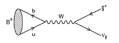
Figure 1: Purely leptonic $B$ decay $B^{+}\rightarrow\ell^{+}\nu_{\ell}$ proceeds via quark annihilation into a $W$ boson.

The decay amplitude is proportional to the lepton mass and decay to the lighter leptons is severely suppressed. This mode is thus the most promising for discovery at existing experiments. However, challenges such as the large missing momentum from several neutrinos make the signature for $B^{+}\rightarrow\tau^{+}\nu_{\tau}$ less distinctive than for other leptonic modes.

The Standard Model estimate of this branching fraction is $7.5\times 10^{-5}$, given the PDG 2002 values for $f_{B}$, $|V_{ub}|$, and the $B^{+}$ lifetime: $f_{B}=198\mathrm{\,Me\kern-1.00006ptV}$, $V_{ub}=0.0036$, $\tau_{B^{+}}=1.674{\rm\,ps}$ [4].

Purely leptonic $B$ decays have not yet been observed. CLEO [5] and experiments at LEP [6][7][8] have searched for this process and set limits on the branching fraction at the 90% confidence level (CL). The most stringent limit on $\mathcal{B}(B^{+}\rightarrow\tau^{+}\nu_{\tau})$ comes from the L3 experiment:

$$\mathcal{B}(B^{+}\rightarrow\tau^{+}\nu_{\tau}) < 5.7\times 10^{-4}\,\textrm{at the 90\% CL }$$ (2)

2 The BABAR Detector and Dataset

The data used in this analysis were collected with the BABAR detector at the PEP-II storage ring. The sample corresponds to an integrated luminosity of $81.9\mbox{\,fb}^{-1}$ at the $\mathchar 28935\relax{(4S)}$ resonance (on-resonance) and $9.58\mbox{\,fb}^{-1}$ taken $40\mathrm{\,Me\kern-1.00006ptV}$ below the $\mathchar 28935\relax{(4S)}$ resonance (off-resonance). The on-resonance sample consists of about 88.9 million $B\kern 1.79993pt\overline{\kern-1.79993ptB}{}$ pairs. The collider is operated with asymmetric beam energies, producing a boost of $\beta\gamma\approx 0.56$ of the $\mathchar 28935\relax{(4S)}$ along the collision axis.

The BABAR detector is described elsewhere [9]. Charged-particle momentum, direction, and energy loss ($\frac{dE}{dx}$) measurements are performed by a five-layer double-sided silicon vertex tracker (SVT) and a 40-layer drift chamber (DCH) which are immersed in the field of a 1.5-T super-conducting solenoid. Charged particle identification is performed by a detector of internally-reflected Cherenkov light (DIRC). The energies of electrons and photons are measured by the electromagnetic calorimeter (EMC) consisting of an array of 6580 CsI(Tl) crystals. The flux return is instrumented with resistive plate chambers (IFR) to detect the passage of muons and neutral hadrons.

A GEANT4-based [10] Monte Carlo (MC) simulation is used to model the signal efficiency and the physics backgrounds. Simulation samples equivalent to approximately three times the accumulated data were used to model $B\kern 1.79993pt\overline{\kern-1.79993ptB}{}$ events, and samples equivalent to approximately 1.5 times the accumulated data were used to model $e^{+}e^{-}\rightarrow$ $u\overline{u}$, $d\overline{d}$, $s\overline{s}$, $c\overline{c}$, and $\tau^{+}\tau^{-}$ events.

3 Analysis Method

3.1 Event Selection

The decay $B^{+}\rightarrow\tau^{+}\nu_{\tau}$  and subsequent one-prong leptonic decays $\tau^{+}\rightarrow e^{+}\nu_{e}\overline{\nu}_{\tau}$ and $\tau^{+}\rightarrow\mu^{+}\nu_{\mu}\overline{\nu}_{\tau}$ lead to the production of a single, visible charged particle and missing energy carried by neutrinos. Therefore, any remaining neutral energy or charged tracks originate from the other $B$. The search for $B^{+}\rightarrow\tau^{+}\nu_{\tau}$ proceeds by reconstructing one of the $B$ mesons in each event in the semi-leptonic topology $B^{-}\rightarrow D^{0}\ell^{-}\bar{\nu}_{\ell}X$ (henceforth referred to as the semi-leptonic side or semi-leptonic B), where $X$ could be a photon, neutral pion, or nothing. The remainder of the event is searched for evidence of the one-prong leptonic $\tau^{+}$ decay modes.

The choice of a semi-exclusive, semi-leptonic $B$ decay means that the $B$ meson cannot be fully reconstructed, since there is a neutrino missing and excited neutral $D$ states are not reconstructed, potentially leaving unassigned neutral energy in the event. The inherent cleanliness of the events (small multiplicity, little unassigned neutral energy), however, is a powerful constraint that compensates for the choice of reconstruction mode. This method has been used in a search for $B^{+}\rightarrow K^{+}\nu\bar{\nu}$ [11].

Events are pre-selected by requiring that their net charge is zero, that $R_{2}<0.9$ (where $R_{2}$ is the normalized second Fox-Wolfram moment [12]), and that they have large missing mass ($M_{miss}>1.0\mathrm{\,Ge\kern-1.00006ptV}$). We select our semi-leptonic side by first reconstructing $D^{0}$ candidates in one of four modes: $D^{0}\rightarrow K^{-}\pi^{+}$, $D^{0}\rightarrow K^{-}\pi^{+}\pi^{0}$, $D^{0}\rightarrow K^{-}\pi^{+}\pi^{+}\pi^{-}$, and $D^{0}\rightarrow K^{0}_{\scriptscriptstyle S}\pi^{+}\pi^{-}$. The $K^{0}_{\scriptscriptstyle S}$ is reconstructed only in the charged mode $K^{0}_{\scriptscriptstyle S}\rightarrow\pi^{+}\pi^{-}$. The $D^{0}$ meson is required to have a momentum in the center-of-mass ($\mathchar 28935\relax{(4S)}$) frame $p^{*}_{D^{0}}>0.5\mathrm{\,Ge\kern-1.00006ptV}$, and its daughters are required to meet particle identification criteria consistent with the particle hypothesis.

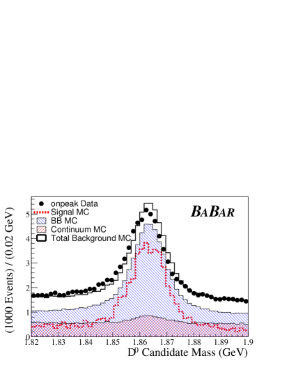
Figure 2: The $D^{0}$ mass distribution after making event preselections and requiring that events have at least one $B^{-}\rightarrow D^{0}\ell^{-}\bar{\nu}_{\ell}X$ candidate. Background MC combines $B\kern 1.79993pt\overline{\kern-1.79993ptB}{}$ (excluding $B^{+}\rightarrow\tau^{+}\nu_{\tau}$ decays) and continuum MC and is normalized to the data area, while the normalization of the signal simulation is arbitrary. Due to the large size of this sample, the data error bars are too small to see in the figure.

We pair the $D^{0}$ candidates with leptons whose momentum in the center-of-mass frame meets the requirement $p_{\ell}^{*}>1.3\mathrm{\,Ge\kern-1.00006ptV}$. The $D^{0}$-lepton pairs are required to converge at a common vertex; these pairs are referred to as $D\ell$ candidates. If there are multiple $D\ell$ candidates in an event we select the candidate whose reconstructed $D^{0}$ mass is closest to the average reconstructed mass for its decay mode. If the best candidate can be paired with a pion to make a $D^{*+}\ell^{-}$ candidate, then the event is consistent with being a $B^{0}\kern 1.79993pt\overline{\kern-1.79993ptB}{}^{0}$ event and is rejected.

The mass distribution for these $D^{0}$ candidates is shown in Fig. 2. There is a difference between the mean of data and the mean of MC because the MC generator uses a $D^{0}$ mass that differs from the PDG value by $1\mathrm{\,Me\kern-1.00006ptV}$. The width of distribution is typically narrower in MC by $0.2\mathrm{\,Me\kern-1.00006ptV}$ ($K^{-}\pi^{+}$) to $4\mathrm{\,Me\kern-1.00006ptV}$ ($K^{-}\pi^{+}\pi^{0}$) due to energy and momentum resolution differences in data and MC. To account for differences in mean position and peak width, we require that the reconstructed $D^{0}$ mass be within $3\sigma$ of the fitted mean for the mode under consideration. The widths of the peaks vary by $D^{0}$ mode, from $3.8\mathrm{\,Me\kern-1.00006ptV}$ for $D^{0}\rightarrow K^{-}\pi^{+}\pi^{-}\pi^{+}$ to $10.4\mathrm{\,Me\kern-1.00006ptV}$ for $D^{0}\rightarrow K^{-}\pi^{+}\pi^{0}$.

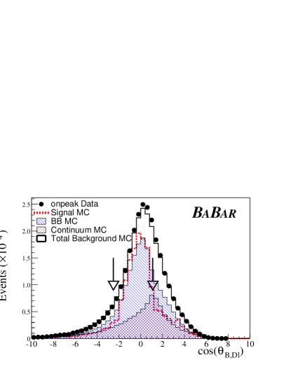
Figure 3: The quantity $\cos{\theta_{B,D\ell}}$, computed from the energies and momenta of the $D\ell$ and the $B$ meson assuming only a neutrino is missing. Background MC combines $B\kern 1.79993pt\overline{\kern-1.79993ptB}{}$ (excluding $B^{+}\rightarrow\tau^{+}\nu_{\tau}$ decays) and continuum MC and is normalized to the data area, while the normalization of the signal simulation is arbitrary. The arrows represent the boundaries of the selection region between $-2.5$ and $1.1$. Due to the large size of this sample, the data error bars are too small to see in the figure.

A restriction is also placed on $\cos{\theta_{B,D\ell}}$, where $\theta_{B,D\ell}$ is computed from $B$ and $D\ell$ momenta and energy in the center-of-mass frame under the assumption that only a neutrino is missing,

$$\cos{\theta_{B,D\ell}}=\frac{(2\,E_{{B}}E_{D\ell}-m^{2}_{{B}}-m^{2}_{D\ell})}{2\,|\vec{p}_{{B}}||\vec{p}_{D\ell}|}\,.$$ (3)

Since the semi-leptonic $B$ cannot be completely reconstructed its energy, $E_{{B}}$, and momentum, $|\vec{p}_{{B}}|$, are derived from the beam energies. The variable $\cos{\theta_{B,D\ell}}$ can take on values outside $(-1,1)$ for events in which particles besides the neutrino have been missed in the semi-leptonic decay. We allow for the feed-down of excited neutral $D$ states into the analysis by applying an asymmetric cut of $-2.5<\cos{\theta_{B,D\ell}}<1.1$. This variable is shown in Fig. 3. Differences in the semi-leptonic side between data and simulation are later corrected (Sec. 4.2) in the overall efficiency estimate.

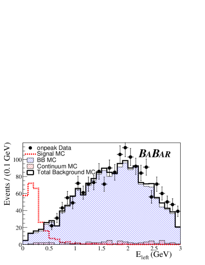
Figure 4: $E_{\mathrm{left}}$, the neutral energy remaining in the calorimeter after excluding neutrals associated with the semi-leptonic side. In the above distribution all analysis selection criteria are applied. The data are not shown below $0.5\mathrm{\,Ge\kern-1.00006ptV}$. The normalization of the signal MC is arbitrary.

Once the semi-leptonic side has been reconstructed, its daughter particles are excluded from the event. Any neutral or charged object that is not associated with the semi-leptonic side is referred to as belonging to the signal side. The event is then required to have only one remaining charged particle with a small impact parameter in the $(r,\phi)$ plane. This track is required to fail kaon identification and be identified either as a muon or an electron. In addition, $\tau^{+}\tau^{-}$ continuum events are rejected by making requirements on the angle of the track with respect to the event thrust axis ($|\cos{\theta_{\vec{p},\vec{T}}}|<0.9$) and the minimum mass capable of being made from any three tracks in the event ($M_{3}^{min}>1.5\mathrm{\,Ge\kern-1.00006ptV}$). In general, continuum events are sharply peaked toward 1.0 in $|\cos{\theta_{\vec{p},\vec{T}}}|$; additionally, $\tau^{+}\tau^{-}$ events tend to have a value of $M_{3}^{min}$ peaked below the $\tau$ mass.

The variable $E_{\mathrm{left}}$, the neutral energy remaining in the calorimeter after excluding neutrals from the semi-leptonic $B$, provides good discrimination between signal and background (Fig. 4). For true signal events, this quantity is peaked toward zero energy while for background it peaks near $2\mathrm{\,Ge\kern-1.00006ptV}$. We make a loose restriction of $E_{\mathrm{left}}<1.0\mathrm{\,Ge\kern-1.00006ptV}$ in preparation for the final step of the analysis, which is to fit the $E_{\mathrm{left}}$ distribution and extract the signal and background contributions.

To minimize experimenter bias, the data were not studied in the signal-populated region of $E_{\mathrm{left}}$ until systematic checks were performed using control samples in the region of $E_{\mathrm{left}}$ ($E_{\mathrm{left}}>0.5\mathrm{\,Ge\kern-1.00006ptV}$) which does not contain a significant signal yield. The region $0.5<E_{\mathrm{left}}<1.0\mathrm{\,Ge\kern-1.00006ptV}$ is defined to be the neutral energy sideband, while the region $E_{\mathrm{left}}<0.5\mathrm{\,Ge\kern-1.00006ptV}$ is referred to as the signal region.

3.2 Selection Efficiency

After applying all selection criteria we obtain a signal efficiency in the Monte Carlo simulation of $(6.99\pm 0.31)\times 10^{-4}$, where the error is purely from the statistics of the signal MC. This number does not include corrections for differences between data and simulation, which will be described in Sec. 4. The number of background events expected for $E_{\mathrm{left}}<1.0\mathrm{\,Ge\kern-1.00006ptV}$, determined from simulation, is $269.1\pm 9.6$, where the error is purely statistical.

3.3 The Limit-Setting Procedure

We fit $E_{\mathrm{left}}$ using an extended maximum likelihood function; from this fit we extract the contributions to the distribution from signal and background events. The likelihood function is of the following form:

$$\mathcal{L}=e^{-(\mu_{s}+\mu_{b})}\prod_{i=1}^{n}\left(\mu_{s}\,F_{s}({E_{\mathrm{left}}}_{i})+\mu_{b}\,F_{b}({E_{\mathrm{left}}}_{i})\right)$$ (4)

where $\mu_{s}$ is the number of signal events, $\mu_{b}$ is the number of background events (both of which are obtained by fitting the selected data sample) and $n$ is the total number of events in the selected sample. The functions $F_{s}({E_{\mathrm{left}}})$ and $F_{b}({E_{\mathrm{left}}})$ are the Probability Density Functions (PDFs) which are obtained from the $E_{\mathrm{left}}$ distributions in signal and background MC. The nominal models for signal and background are shown in Fig. 5.

The $E_{\mathrm{left}}$ distribution in the signal MC has several salient features. The peak at $200\mathrm{\,Me\kern-1.00006ptV}$ arises from the unassigned photon or $\pi^{0}$ daughter of a $D^{*0}$  on the semi-leptonic side. The peak at zero energy arises from events without remaining neutral energy, and above zero the spectrum falls exponentially under the peak from the $D^{*0}$ neutrals, the result of neutrals in the MC arising from beam background and hadronic split-offs.

The background PDF is a second-order polynomial rising monotonically between $0\mathrm{\,Ge\kern-1.00006ptV}$ and $1.0\mathrm{\,Ge\kern-1.00006ptV}$. An estimate of the background from data is determined by extrapolating the data $E_{\mathrm{left}}$ sideband into the signal region using the background PDF. The result is a background estimate of $273.6\pm 19.2$ events.

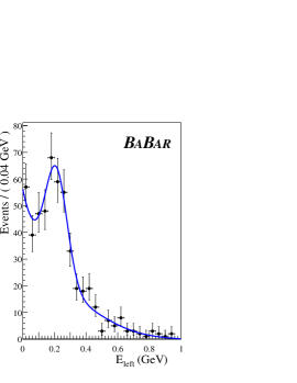
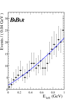
Figure 5: The signal PDF (left) fitted to $E_{\mathrm{left}}$ from the signal MC and the background PDF (right) fitted to $E_{\mathrm{left}}$ from the background MC. All selection criteria are applied to the events in signal and background MC. The normalization of the signal MC is arbitrary and the normalization of the background MC is fixed to the integrated luminosity.

To determine the 90% confidence limit, denoted $\mu_{s}^{90}$, for the measured value of $\mu_{s}$ we use a modified frequentist approach based on that used by the LEP experiments in the Higgs search [14]. This approach constructs an estimator based on the fitted signal yield, $\mu_{s}^{fitted}$. In all following discussions, toy MC refers to $E_{\mathrm{left}}$ spectra obtained by randomly sampling the signal and background $E_{\mathrm{left}}$ PDFs and treating the samples as a data set. The limit-setting method is outlined as follows:

1. Toy MC experiments are generated with our expected number of background events and a signal hypothesis, $\mu_{s}^{input}=\mu_{s}^{expected}$. Each toy experiment is fitted for the signal yield, $\mu_{s}^{\prime}$. The collection of $\mu_{s}^{\prime}$ forms a distribution. We denote the normalized fitted signal distribution for the original signal hypothesis as $D_{s+b}(\mu_{s}^{\prime},\mu_{s}^{input})$.

2. Toy MC is also generated with a signal hypothesis of zero events and with the expected number of background events. Again, each data sample is fitted and we obtain the distribution of the fitted signal yield. We denote the normalized distribution of the fitted signal yield in the null signal hypothesis as $D_{b}(\mu_{s}^{\prime})$.

3. For a specific data sample, a fit is performed using the likelihood function to obtain the number of signal events in the sample, $\mu_{s}^{fitted}$. The confidence level (CL) for this measurement, for a signal hypothesis $\mu_{s}^{expected}$, is given by:

   $$CL(\mu_{s}^{fitted},\mu_{s}^{expected})\equiv\frac{\int_{-\infty}^{\mu_{s}^{fitted}}D_{s+b}(\mu_{s}^{\prime};\mu_{s}^{expected})d\mu_{s}^{\prime}}{\int_{-\infty}^{\mu_{s}^{fitted}}D_{b}(\mu_{s}^{\prime})d\mu_{s}^{\prime}}$$ (5)

4. The 90% confidence limit corresponding to this fitted signal yield, $\mu_{s}^{fitted}$, is defined by the requirement:

   $$CL(\mu_{s}^{fitted},\mu_{s}^{90}) = 1-0.90$$ (6)

   A scan is performed over signal hypotheses until the minimum signal hypothesis which satisfies the requirement is determined. This signal hypothesis is $\mu_{s}^{90}$. The relationship between $\mu_{s}^{90}$ and $\mu_{s}^{fitted}$ is given in Fig. 6.

We use the background-only hypothesis to determine the nominal sensitivity for the analysis. The nominal background PDF is used to generate 10,000 toy MC experiments, each with a total number of events Poisson-distributed around the nominal background expectation of $269\pm 9.6$ events. The $E_{\mathrm{left}}$ distribution so generated for each experiment is fitted with the likelihood function, and the curve in Fig. 6 is used to obtain the corresponding $\mu_{s}^{90}$. The distribution of $\mu_{s}^{90}$ for these toy experiments is shown in Fig. 6, and the median of this distribution provides our nominal sensitivity, $\mu_{s}^{90}=15.4$.

A test of the method is performed using two independent samples of GEANT4 MC, each with a total luminosity equal to that of the data set. Each simulated experiment contains only background events and has all analysis selection criteria applied. The results obtained from fitting these two experiments, $\mu_{s}^{90}=13.3$ and $\mu_{s}^{90}=19.4$ are in good agreement with the nominal sensitivity and are illustrated in Fig. 6. The results of these GEANT4 MC experiments are used in Sec. 4.1 to explore potential systematic effects on the limit-setting procedure.

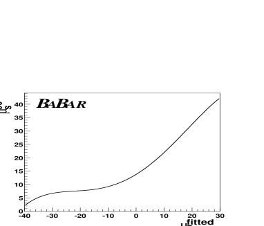
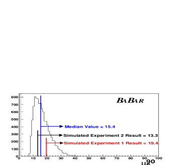
Figure 6: The relationship between $\mu_{s}^{90}$ and $\mu_{s}^{fitted}$ is shown in the left figure. In the right figure is the distribution of $\mu_{s}^{90}$ obtained from fitting 10,000 toy MC experiments generated using the null signal hypothesis. The black line indicates the median of this distribution, which is taken as the nominal sensitivity of the analysis ($\mu_{s}^{90}=15.4$). The red and blue lines indicate the results of applying the analysis to two independent, background-only GEANT4 MC experiments.

The strength of this method is that it takes full advantage of the information contained in the shape of the signal and background and is insensitive to the absolute background normalization. It relies on the accuracy of the simulation, in particular the simulation of the calorimeter for low neutral cluster energy. The systematic effects on the limit-setting procedure, as well as on the signal efficiency, are discussed in the next section.

4 Evaluation of Systematic Uncertainties

In this section we discuss the systematic uncertainties affecting the limit-setting procedure and the calculation of the efficiency.

4.1 Systematic Effects for Limit-Setting

Table 1 lists the sources of systematic uncertainty and their effects on the overall expected sensitivity of a pair of independent “experiments” derived from the background MC sample. Since MC is used to generate the PDFs for signal and background, effects of concern are those which might cause the true background or signal distributions to differ from the simulation. For each source of potential systematic uncertainty listed below, a CL curve is calculated (as in Fig. 6) by generating toy MC with a systematically modified model and fitting with the nominal model.

To explore the potential differences between data and MC when validating the background PDF, several control samples have been developed by performing the semi-leptonic reconstruction on data and MC and applying selection criteria to the remainder of the event:

• ($B^{-}\rightarrow D^{0}\ell^{-}\bar{\nu}_{\ell}X$) + (anything): The $B^{-}\rightarrow D^{0}\ell^{-}\bar{\nu}_{\ell}X$ reconstruction algorithm is applied and no restrictions are placed on the signal side.

• ($B^{0}\rightarrow D^{*+}\ell^{-}\nu$) + (1 track) : The semi-leptonic reconstruction algorithm is applied, but semi-leptonic candidates are kept where the best candidate is reconstructed as a $D^{*+}\ell^{-}\nu$. We then require only one track remaining in the event. This sample has a topology similar to the signal sample.

• ($B^{-}\rightarrow D^{0}\ell^{-}\bar{\nu}_{\ell}X$) + (2 tracks): The $B^{-}\rightarrow D^{0}\ell^{-}\bar{\nu}_{\ell}X$ reconstruction algorithm is applied and the signal side is required to contain exactly two charged tracks. This requirement enforces a mis-reconstructed signal side, since total event charge is non-zero.

The difference between data and simulation for each of these samples is used to construct a correction function for the PDFs. The PDFs are multiplied by the correction function and re-normalized. The upper limit is recalculated using the corrected PDFs to generate the toy MC samples discussed in Sec. 3, while fitting is still performed with the nominal model. The results of this study are given in Table 1.

Motivated by the data/MC yield disagreement in the control samples, we explored the effects of a significant difference between the actual background and the background expectation. Given the expected background from MC ($269.1\pm 9.6$ events), we varied the input background hypothesis to our toy MC by $\pm 10$ and $\pm 20$ events and used the nominal likelihood function to generate CL curves for each case. The result was a change in the nominal sensitivity of $\mu_{s}^{90}$ of no more than $0.5$ events (Table 1). Therefore we concluded that if the actual background in data is different than the expectation from MC, the resulting change in the limit is small.

The choice of background parametrization has also been explored as a possible effect on the limit-setting procedure. Different models (second-order polynomial, Gaussian tail, KEYS [13], histogram) were used to represent the background $E_{\mathrm{left}}$ spectrum and then generate toy MC. These toy samples were again fitted with the nominal model and the variation in the confidence limit curve was explored. The results are given in Table 1. Limit curves calculated from this variation in the background model yielded a lower limit on the signal yield, suggesting that the second-order polynomial leads to a conservative limit.

A feature at or near zero energy in the $E_{\mathrm{left}}$ spectrum, unmodelled in the Monte Carlo, is another possible effect in the background that could fake a signal. Such a feature is suggested by studying the $B^{0}\rightarrow D^{*+}\ell^{-}\nu$ + 1 track control sample, which suggested a maximal difference near zero energy in data and MC of a factor of two. To explore the effect of such a feature, toy MC is generated with the background PDF enhanced by a factor of two near zero. This toy MC is then fit using the nominal signal and background models to study the variation in the confidence limit. The results are given in Table 1.

To validate the signal PDF, a control sample of $B^{-}\rightarrow D^{0}\ell^{-}\bar{\nu}_{\ell}X$,$B^{+}\rightarrow\kern 1.99997pt\overline{\kern-1.99997ptD}{}^{*0}\ell^{+}\nu_{\ell}$ is used to check the difference between data and simulation after making all semi-leptonic and signal-side requirements. This sample has a semi-leptonic side as in the signal analysis, and a signal side which is also reconstructed as an independent $B^{+}\rightarrow\kern 1.99997pt\overline{\kern-1.99997ptD}{}^{0}\ell^{+}\nu_{\ell}X$. We then construct a subsample of these events where a photon or $\pi^{0}$ could be associated with the $\kern 1.99997pt\overline{\kern-1.99997ptD}{}^{0}$ on the signal side to make a $\kern 1.99997pt\overline{\kern-1.99997ptD}{}^{*0}$. Having attempted to account for the neutral from $\kern 1.99997pt\overline{\kern-1.99997ptD}{}^{*0}$ decay on the signal side, the neutral energy spectrum should resemble that for signal events. However, this subsample has more neutral energy present from hadronic splitoffs, and the correct photon or $\pi^{0}$ is not always associated with the $\kern 1.99997pt\overline{\kern-1.99997ptD}{}^{0}$ to make the $\kern 1.99997pt\overline{\kern-1.99997ptD}{}^{*0}$. Therefore, a comparison is made between data and the corresponding MC sample and not between data and signal MC. The sample suggests that there may be a difference of $\sim 20\mathrm{\,Me\kern-1.00006ptV}$ in the overall position of the peak near $200\mathrm{\,Me\kern-1.00006ptV}$. The effects of such a difference are given in Table 1.

Table 1: Sources of potential systematic uncertainty have been explored and their effects on the expectation for $\mu_{s}^{90}$ observed. The simulated experiments come from two independent samples of full MC, each with luminosity equivalent to the data luminosity. Despite the many potential differences between data and simulation, the variation in the upper limit is small copared to the variation of limit expected for the zero signal hypothesis.

Systematic Variation	Control Sample used	$\mu_{s}^{90}$	$\mu_{s}^{90}$
	to guide the variation	Simulated	Simulated
		Experiment 1	Experiment 2
None (Nominal Model)	None	19.4	13.3
Data/Simulation	$B^{-}\rightarrow D^{0}\ell^{-}\bar{\nu}_{\ell}X$ + anything	18.0	12.4
Shape Difference	$B^{0}\rightarrow D^{*+}\ell^{-}\nu$ + 1 track	18.6	13.0
	$B^{-}\rightarrow D^{0}\ell^{-}\bar{\nu}_{\ell}X$ + 2 tracks	17.8	12.2
Incorrect Background Estimate
-20 Events		19.0	12.0
-10 Events	All	19.3	13.1
+10 Events		19.7	13.6
+20 Events		19.8	13.7
Gaussian Tail Background Model	None	17.1	12.0
KEYS Background Model	None	17.4	12.0
Histogram Background Model	None	17.2	11.8
Factor of 2
enhancement in	$B^{0}\rightarrow D^{*+}\ell^{-}\nu$ + 1 track	16.5	11.5
background near
$E_{\mathrm{left}}=0.0\mathrm{\,Ge\kern-1.00006ptV}$
$+20\mathrm{\,Me\kern-1.00006ptV}$ Shift in
Signal PDF Gaussian	$B^{-}\rightarrow D^{0}\ell^{-}\bar{\nu}_{\ell}X$,$B^{+}\rightarrow\kern 1.99997pt\overline{\kern-1.99997ptD}{}^{*0}\ell^{+}\nu_{\ell}$	20.2	13.9
$-20\mathrm{\,Me\kern-1.00006ptV}$ Shift in
Signal PDF Gaussian	$B^{-}\rightarrow D^{0}\ell^{-}\bar{\nu}_{\ell}X$,$B^{+}\rightarrow\kern 1.99997pt\overline{\kern-1.99997ptD}{}^{*0}\ell^{+}\nu_{\ell}$	18.9	13.0

In almost all cases that were investigated, the nominal model yields the most conservative CL curve. Additionally, the variation in the upper limit expectation is small compared to the overall variation of the limit for the zero signal hypothesis. We therefore use the nominal model to set the limit, having determined that the systematic effects mentioned above have negligible impact on the result.

4.2 Systematic Effects for Signal Efficiency

The efficiency calculated in Sec. 3.2 needs to be corrected for differences in data and MC. The effects of several systematic uncertainty have been evaluated. The results are expressed in a correction factor and a systematic error associated with the correction. The most prominent sources of systematic uncertainties are listed in Table 2.

Table 2: The corrections which are applied in this analysis on the signal efficiency, as well as the error associated with each correction.

Source	Correction Factor	Correction Error
B-Counting	1.0	0.011
Semi-Leptonic
Reconstruction Efficiency	0.958	0.051
Neutral Energy	1.0	0.025
Tracking Efficiency
(signal track only)	1.0	0.008
Particle ID
(signal track only)	0.836	0.042
Total	0.801	0.063

The semi-leptonic reconstruction efficiency correction is evaluated by using a sample of $N_{2}$ double-reconstruction events ($B^{-}\rightarrow D^{0}\ell^{-}\bar{\nu}_{\ell}X$, $B^{+}\rightarrow\kern 1.99997pt\overline{\kern-1.99997ptD}{}^{0}\ell^{+}\nu_{\ell}X$) and a sample of $N_{1}$ single-reconstruction events in the same data set, where the single-reconstruction sample excludes double-reconstructed events. To isolate the effects of the semi-leptonic reconstruction, we remove the event preselection requirements which are unrelated to the selection of the semi-leptonic decay. The ratio of the sizes of these two samples is given by:

$$\frac{N_{1}}{N_{2}} = \frac{2(1-\varepsilon)}{\varepsilon}$$ (7)

where $\varepsilon$ is the probability of selecting a second $B$ meson in the mode $B^{-}\rightarrow D^{0}\ell^{-}\bar{\nu}_{\ell}X$ having already selected one $B$ meson in that mode. Equation 7 is solved for $\varepsilon$, and the ratio of $\varepsilon$ in data and simulation is taken as a correction on the efficiency,

$$\frac{\varepsilon_{data}}{\varepsilon_{MC}} = 0.958\pm 0.051\,.$$ (8)

The correction of the signal efficiency due to particle identification (PID) is performed as follows. Using control samples of electrons and muons from data, the performance of the kaon veto and lepton identification is evaluated as a function of lab momentum ($p$) and polar angle ($\theta$). This performance translates into a weight for an identified track with a given momentum. Integrating this weight over the momentum spectrum of the signal MC for true one-prong leptonic $\tau^{+}$ decays provides the efficiency of the selection in data.

The efficiency in the MC is evaluated by comparing the true identity of a $\tau^{+}$ daughter to the reconstructed identity. The ratio of the data efficiency to the MC efficiency is taken as the signal efficiency correction from particle identification. The statistical uncertainties on the signal MC sample size and PID weights translate into a systematic error on the correction. This error is dominated by the signal MC sample size.

We apply the total correction listed in Table 2 to the signal efficiency from MC to obtain the signal efficiency, $(5.60\pm 0.25(stat.)\pm 0.44(syst.))\times 10^{-4}$. The uncertainty on each correction is propagated through to a systematic error on the signal efficiency, while the statistical uncertainty derives from the signal MC sample size.

Systematic uncertainty is incorporated into the branching fraction limit as follows: for each branching fraction hypothesis, the corresponding signal hypothesis is determined by sampling 10,000 times from a Gaussian distribution about the mean of the signal efficiency, where the width of the Gaussian is given by the systematic error on the signal efficiency. From each signal hypothesis a toy MC experiment is generated and fitted using the likelihood function. This is repeated for many branching fraction hypotheses and the CL curve, including systematic error, is calculated.

5 Results

We apply all selection criteria in the analysis and fit the $E_{\mathrm{left}}$ spectrum in the data below $1.0\mathrm{\,Ge\kern-1.00006ptV}$ using the nominal likelihood function. The result of the fit is given in Table 3 and shown in Fig. 7.

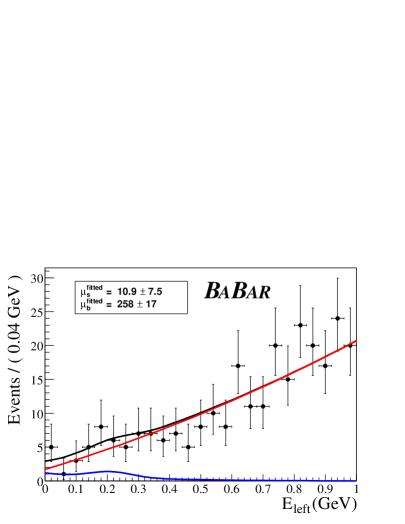
Figure 7: The $E_{\mathrm{left}}$ spectrum in data from zero to $1.0\mathrm{\,Ge\kern-1.00006ptV}$ and the fit of the likelihood function to the spectrum.

Table 3: The results of the fit of the likelihood function to data is given below.

Fit Parameter	Fitted Value
$\mu_{s}^{fitted}$	$10.9\pm 7.5$
$\mu_{b}^{fitted}$	$258\pm 17$

The background yield of $258\pm 17$ is in agreement with the expectation from extrapolating sideband data into the $E_{\mathrm{left}}$ signal region, $274\pm 19$.

We apply our confidence limit curve to the fitted number of signal events (Fig. 6) and determine the 90% confidence limit on the signal yield to be

$$\mu_{s}^{90} = 22.8,$$ (9)

which yields a limit on the branching fraction at the 90% confidence level of

$$\mathcal{B}(B^{+}\rightarrow\tau^{+}\nu_{\tau}) < 4.6\times 10^{-4}\,\textrm{at the 90\% CL}$$ (10)

where we have assumed equal production of $B^{+}B^{-}$ and $B^{0}\kern 1.79993pt\overline{\kern-1.79993ptB}{}^{0}$ at the $\mathchar 28935\relax{(4S)}$ resonance. The expectation from studies in MC containing zero signal events was given in Sec. 3 as $\mu_{s}^{90}=15.4$; the comparison of the expected sensitivity and the measured result is shown in Fig. 8.

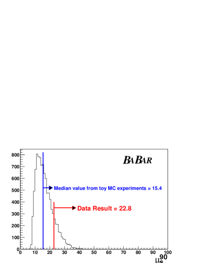
Figure 8: The nominal sensitivity (15.4), obtained from the median of 10,000 toy MC experiments, is compared to the result from data (22.8).

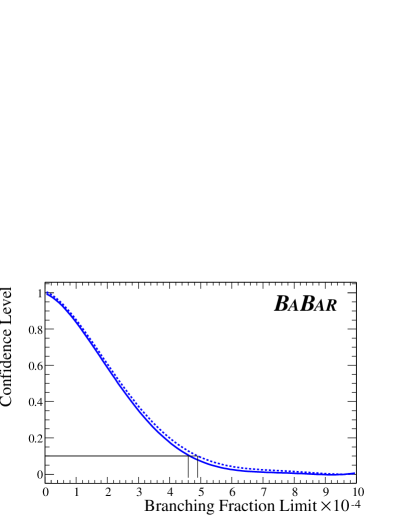
Figure 9: The relationship between the confidence level and the branching fraction limit both in the case where systematic error is (dashed) and is not (solid) incorporated. Lines are drawn at the locations of the 90% confidence limits for both cases.

After incorporating the systematic uncertainty on the signal efficiency (Fig. 9) we find an upper limit on the branching fraction of

$$\mathcal{B}(B^{+}\rightarrow\tau^{+}\nu_{\tau}) < 4.9\times 10^{-4}\,\textrm{at the 90\% CL}$$ (11)

A separate BABAR analysis to search for $B^{+}\rightarrow\tau^{+}\nu_{\tau}$ has also been performed where $B$ mesons are resonstructed via the semi-exclusive hadronic modes $B^{-}\rightarrow D^{(*)0}X^{-}$, where $X^{-}$ represents a combination of up to five charged pions or kaons and up to two $\pi^{0}$ candidates. The semi-exclusive hadronic reconstruction analysis is statistically independent of the present work and has obtained the limit [15]

$$\mathcal{B}(B^{+}\rightarrow\tau^{+}\nu_{\tau})<7.7\times 10^{-4}\,\textrm{at the 90\% CL}$$ (12)

The results of this statistically independent analysis are combined with that reported here using the same modified frequentist method. For each analysis, 5000 toy MC experiments are generated each for a branching fraction hypothesis between $1\times 10^{-4}$ and $10\times 10^{-4}$ in steps of $2.5\times 10^{-6}$. The number of events in each toy experiment that contains signal and background is denoted $n_{(s+b)}$. For each branching fraction hypothesis a separate sample of 5000 background-only toy experiments is also generated; the number of events in a given experiment in this sample is denoted $n_{(b)}$. For a given hypothesis $i$ (where $i=(s+b)$, $(b)$, or $data$) the likelihood estimators, $Q_{i}$, are calculated in each toy experiment:

$$Q_{i} = \frac{\mathcal{L}(n_{i}|s+b)}{\mathcal{L}(n_{i}|b)}$$ (13)

where $\mathcal{L}(n_{i}|s+b)$ is the likelihood of a given toy experiment with $n_{i}$ events being consistent with the $(s+b)$ hypothesis (in equation 4, $\mu_{s}$ is set to the number of signal $s$, corresponding to the branching fraction hypothesis, and $\mu_{b}$ is set to the number of background $b$). Systematic errors are incorporated by each analysis into the $Q_{i}$. They are combined as follows:

$$Q_{i}^{\textrm{combined}} = Q_{i}^{\textrm{semi-leptonic}}\times Q_{i}^{\textrm{hadronic}}.$$ (14)

The confidence level for a particular branching ratio hypothesis is given by counting the number of experiments, $N_{(Q_{i}<Q_{data})}$, that have a value of $Q_{(s+b)}$ ($Q_{(b)}$) less than that for data ($Q_{data}$) and taking the ratio

$$CL_{s} = \frac{N_{({Q_{(s+b)}<Q_{data}})}}{N_{({Q_{(b)}<Q_{data}})}}.$$ (15)

From this a combined BABAR result is obtained:

$$\mathcal{B}(B^{+}\rightarrow\tau^{+}\nu_{\tau})_{combined}<4.1\times 10^{-4}\,\textrm{at the 90\% CL}.$$ (16)

6 Summary

We have performed a search for the decay process $B^{+}\rightarrow\tau^{+}\nu_{\tau}$. To accomplish this a sample of semi-leptonic $B$ decays ($B^{-}\rightarrow D^{0}\ell^{-}\bar{\nu}_{\ell}X$) has been used to reconstruct one of the $B$ mesons and the remaining information in the event is searched for evidence of $B^{+}\rightarrow\tau^{+}\nu_{\tau}$. We find no evidence for this decay process and set a preliminary limit on its branching fraction of

$$\mathcal{B}(B^{+}\rightarrow\tau^{+}\nu_{\tau}) < 4.9\times 10^{-4}\,\textrm{at the 90\% CL}$$

By combining this analysis with a statistically independent $B^{+}\rightarrow\tau^{+}\nu_{\tau}$ search performed using a semi-exclusive $B$ reconstruction we find the preliminary combined limit:

$$\mathcal{B}(B^{+}\rightarrow\tau^{+}\nu_{\tau})_{combined}<4.1\times 10^{-4}\,\textrm{at the 90\% CL}$$

7 Acknowledgments

We are grateful for the extraordinary contributions of our PEP-II colleagues in achieving the excellent luminosity and machine conditions that have made this work possible. The success of this project also relies critically on the expertise and dedication of the computing organizations that support BABAR. The collaborating institutions wish to thank SLAC for its support and the kind hospitality extended to them. This work is supported by the US Department of Energy and National Science Foundation, the Natural Sciences and Engineering Research Council (Canada), Institute of High Energy Physics (China), the Commissariat à l’Energie Atomique and Institut National de Physique Nucléaire et de Physique des Particules (France), the Bundesministerium für Bildung und Forschung and Deutsche Forschungsgemeinschaft (Germany), the Istituto Nazionale di Fisica Nucleare (Italy), the Foundation for Fundamental Research on Matter (The Netherlands), the Research Council of Norway, the Ministry of Science and Technology of the Russian Federation, and the Particle Physics and Astronomy Research Council (United Kingdom). Individuals have received support from the A. P. Sloan Foundation, the Research Corporation, and the Alexander von Humboldt Foundation.

References

- [1] W.-S. Hou, Phys. Rev. D 48 (1993) 2342.
- [2] N. Cabbibo, Phys. Rev. Lett. 10, (1963) 531.
- [3] M. Kobayashi and T. Maskawa, Prog. Th. Phys. 49, (1972) 652.
- [4] Particle Data Group, K. Hagiwara et al., Phys. Rev. D66, (2002) 010001.
- [5] CLEO Collaboration, T. E. Browder et al., “A Search for ”, Phys. Rev. Lett. 86, (2001) 2950.
- [6] L3 Collaboration, M Acciarri et al., Phys. Lett. B 396, (1997) 327.
- [7] ALEPH Collaboration, D. Buskulic et al., Phys. Lett. B 343, (1995) 444.
- [8] DELPHI Collaboration, P Abreu et al., Phys. Lett. B 496, (2000) 43.
- [9] BABAR Collaboration, B. Aubert et al., Nucl. Instr. Meth. A 479, (2002) 1.
- [10] S. Agostinelli et al., “Geant4 - A Simulation Toolkit”. SLAC-PUB-9350. Submitted to Nucl. Instr. Meth. A .
- [11] BABAR Collaboration, B. Auber et al., “A Search for ”. SLAC-PUB-9309, BABAR-CONF-02-027.
- [12] G.C Fox and S. Wolfram, Phys. Rev. Lett. 75, 785 (1995).
- [13] K. Cranmer, “Kernel Estimation in High-Energy Physics”, hep-ex/0011057.
- [14] A. L. Read, “Modified frequentist analysis of search results (the method)”, CERN-OPEN-2000-205.
- [15] BABAR Collaboration, B. Aubert et al., “A Search for Using a Fully Reconstructed Sample”, BABAR-CONF-03/004.