Neutral B meson oscillations in the
and
systems were studied using a sample of about 4.0 million
hadronic Z decays recorded by the DELPHI detector between 1992 and 2000.
Events with a high transverse momentum lepton were removed and
a sample of 770 k events with an inclusively reconstructed vertex
was selected.
The mass difference between the two physical states in the
system
was measured to be:
.
The following limit on the width difference of these states was also obtained:
at 95% CL.
As no evidence for
oscillations was found, a limit on the
mass difference of the two physical states was given:
at 95 % CL.
The corresponding sensitivity of this analysis is equal to 6.6 ps-1.
11footnotetext: Department of Physics and Astronomy, Iowa State
University, Ames IA 50011-3160, USA
22footnotetext: Physics Department, Universiteit Antwerpen,
Universiteitsplein 1, B-2610 Antwerpen, Belgium
and IIHE, ULB-VUB,
Pleinlaan 2, B-1050 Brussels, Belgium
and Faculté des Sciences,
Univ. de l’Etat Mons, Av. Maistriau 19, B-7000 Mons, Belgium
33footnotetext: Physics Laboratory, University of Athens, Solonos Str.
104, GR-10680 Athens, Greece
44footnotetext: Department of Physics, University of Bergen,
Allégaten 55, NO-5007 Bergen, Norway
55footnotetext: Dipartimento di Fisica, Università di Bologna and INFN,
Via Irnerio 46, IT-40126 Bologna, Italy
66footnotetext: Centro Brasileiro de Pesquisas Físicas, rua Xavier Sigaud 150,
BR-22290 Rio de Janeiro, Brazil
and Depto. de Física, Pont. Univ. Católica,
C.P. 38071 BR-22453 Rio de Janeiro, Brazil
and Inst. de Física, Univ. Estadual do Rio de Janeiro,
rua São Francisco Xavier 524, Rio de Janeiro, Brazil
77footnotetext: Collège de France, Lab. de Physique Corpusculaire, IN2P3-CNRS,
FR-75231 Paris Cedex 05, France
88footnotetext: CERN, CH-1211 Geneva 23, Switzerland
99footnotetext: Institut de Recherches Subatomiques, IN2P3 - CNRS/ULP - BP20,
FR-67037 Strasbourg Cedex, France
1010footnotetext: Now at DESY-Zeuthen, Platanenallee 6, D-15735 Zeuthen, Germany
1111footnotetext: Institute of Nuclear Physics, N.C.S.R. Demokritos,
P.O. Box 60228, GR-15310 Athens, Greece
1212footnotetext: FZU, Inst. of Phys. of the C.A.S. High Energy Physics Division,
Na Slovance 2, CZ-180 40, Praha 8, Czech Republic
1313footnotetext: Dipartimento di Fisica, Università di Genova and INFN,
Via Dodecaneso 33, IT-16146 Genova, Italy
1414footnotetext: Institut des Sciences Nucléaires, IN2P3-CNRS, Université
de Grenoble 1, FR-38026 Grenoble Cedex, France
1515footnotetext: Helsinki Institute of Physics, HIP,
P.O. Box 9, FI-00014 Helsinki, Finland
1616footnotetext: Joint Institute for Nuclear Research, Dubna, Head Post
Office, P.O. Box 79, RU-101 000 Moscow, Russian Federation
1717footnotetext: Institut für Experimentelle Kernphysik,
Universität Karlsruhe, Postfach 6980, DE-76128 Karlsruhe,
Germany
1818footnotetext: Institute of Nuclear Physics,Ul. Kawiory 26a,
PL-30055 Krakow, Poland
1919footnotetext: Faculty of Physics and Nuclear Techniques, University of Mining
and Metallurgy, PL-30055 Krakow, Poland
2020footnotetext: Université de Paris-Sud, Lab. de l’Accélérateur
Linéaire, IN2P3-CNRS, Bât. 200, FR-91405 Orsay Cedex, France
2121footnotetext: School of Physics and Chemistry, University of Lancaster,
Lancaster LA1 4YB, UK
2222footnotetext: LIP, IST, FCUL - Av. Elias Garcia, 14-,
PT-1000 Lisboa Codex, Portugal
2323footnotetext: Department of Physics, University of Liverpool, P.O.
Box 147, Liverpool L69 3BX, UK
2424footnotetext: LPNHE, IN2P3-CNRS, Univ. Paris VI et VII, Tour 33 (RdC),
4 place Jussieu, FR-75252 Paris Cedex 05, France
2525footnotetext: Department of Physics, University of Lund,
Sölvegatan 14, SE-223 63 Lund, Sweden
2626footnotetext: Université Claude Bernard de Lyon, IPNL, IN2P3-CNRS,
FR-69622 Villeurbanne Cedex, France
2727footnotetext: Dipartimento di Fisica, Università di Milano and INFN-MILANO,
Via Celoria 16, IT-20133 Milan, Italy
2828footnotetext: Dipartimento di Fisica, Univ. di Milano-Bicocca and
INFN-MILANO, Piazza della Scienza 2, IT-20126 Milan, Italy
2929footnotetext: IPNP of MFF, Charles Univ., Areal MFF,
V Holesovickach 2, CZ-180 00, Praha 8, Czech Republic
3030footnotetext: NIKHEF, Postbus 41882, NL-1009 DB
Amsterdam, The Netherlands
3131footnotetext: National Technical University, Physics Department,
Zografou Campus, GR-15773 Athens, Greece
3232footnotetext: Physics Department, University of Oslo, Blindern,
NO-0316 Oslo, Norway
3333footnotetext: Dpto. Fisica, Univ. Oviedo, Avda. Calvo Sotelo
s/n, ES-33007 Oviedo, Spain
3434footnotetext: Department of Physics, University of Oxford,
Keble Road, Oxford OX1 3RH, UK
3535footnotetext: Dipartimento di Fisica, Università di Padova and
INFN, Via Marzolo 8, IT-35131 Padua, Italy
3636footnotetext: Rutherford Appleton Laboratory, Chilton, Didcot
OX11 OQX, UK
3737footnotetext: Dipartimento di Fisica, Università di Roma II and
INFN, Tor Vergata, IT-00173 Rome, Italy
3838footnotetext: Dipartimento di Fisica, Università di Roma III and
INFN, Via della Vasca Navale 84, IT-00146 Rome, Italy
3939footnotetext: DAPNIA/Service de Physique des Particules,
CEA-Saclay, FR-91191 Gif-sur-Yvette Cedex, France
4040footnotetext: Instituto de Fisica de Cantabria (CSIC-UC), Avda.
los Castros s/n, ES-39006 Santander, Spain
4141footnotetext: Inst. for High Energy Physics, Serpukov
P.O. Box 35, Protvino, (Moscow Region), Russian Federation
4242footnotetext: J. Stefan Institute, Jamova 39, SI-1000 Ljubljana, Slovenia
and Laboratory for Astroparticle Physics,
Nova Gorica Polytechnic, Kostanjeviska 16a, SI-5000 Nova Gorica, Slovenia,
and Department of Physics, University of Ljubljana,
SI-1000 Ljubljana, Slovenia
4343footnotetext: Fysikum, Stockholm University,
Box 6730, SE-113 85 Stockholm, Sweden
4444footnotetext: Dipartimento di Fisica Sperimentale, Università di
Torino and INFN, Via P. Giuria 1, IT-10125 Turin, Italy
4545footnotetext: INFN,Sezione di Torino, and Dipartimento di Fisica Teorica,
Università di Torino, Via P. Giuria 1,
IT-10125 Turin, Italy
4646footnotetext: Dipartimento di Fisica, Università di Trieste and
INFN, Via A. Valerio 2, IT-34127 Trieste, Italy
and Istituto di Fisica, Università di Udine,
IT-33100 Udine, Italy
4747footnotetext: Univ. Federal do Rio de Janeiro, C.P. 68528
Cidade Univ., Ilha do Fundão
BR-21945-970 Rio de Janeiro, Brazil
4848footnotetext: Department of Radiation Sciences, University of
Uppsala, P.O. Box 535, SE-751 21 Uppsala, Sweden
4949footnotetext: IFIC, Valencia-CSIC, and D.F.A.M.N., U. de Valencia,
Avda. Dr. Moliner 50, ES-46100 Burjassot (Valencia), Spain
5050footnotetext: Institut für Hochenergiephysik, Österr. Akad.
d. Wissensch., Nikolsdorfergasse 18, AT-1050 Vienna, Austria
5151footnotetext: Inst. Nuclear Studies and University of Warsaw, Ul.
Hoza 69, PL-00681 Warsaw, Poland
5252footnotetext: Fachbereich Physik, University of Wuppertal, Postfach
100 127, DE-42097 Wuppertal, Germany
† deceased
1 Introduction
In the Standard Model, ()
mixing is a
direct consequence of second order weak interactions. Starting with a
meson produced at time =0, the probability density
to observe a
decaying at the proper time can be written, neglecting
effects from CP violation:
.
Here , ,
and , where and denote respectively the heavy
and light physical states.
The oscillation period gives a direct measurement of the mass difference between
the two physical states. The
Standard Model predicts that [1]. Neglecting a possible
difference
between the lifetimes
of the heavy and light mass eigenstates, the above expression simplifies to:
(1)
and similarly:
(2)
where is the lifetime of the B.
In the Standard Model,
the ()
mass difference (having kept
only the dominant top quark contribution) can be expressed as follows [1]:
(3)
In this expression is the Fermi coupling constant; , with
, results from the evaluation of the box diagram and
has a smooth dependence on .
is a QCD correction factor obtained at next-to-leading order
in perturbative QCD.
The dominant uncertainties in Eq.(3) come from
the evaluation of the B meson decay constant and of the “bag”
parameter [2].
In terms of the Wolfenstein parametrization [3], the two elements of
the matrix are equal to:
(4)
neglecting terms of order . At this order is
independent of and
and is equal to .
Eq. (3)
relates to . It defines
a circle in the plane.
Nevertheless the precision on
cannot be fully exploited due to the large uncertainty
which originates in the evaluation of the non-perturbative QCD parameters.
The ratio between the Standard Model expectations for and is given
by:
(5)
A measurement or a limit on the ratio gives a circular constraint
in the plane. This ratio depends only on the ratio of the
non-perturbative QCD parameters which is expected to be better determined than
their absolute values which occur in Eq. (3).
Using constraints on and from existing measurements
(except those on ), the distribution for
the expected values of
can be obtained. It has been shown that should lie,
at 95 C.L., between 9.7 and 23.2 ps-1[2].
Using the DELPHI data, several analyses searching for
oscillations have been performed on selected event samples of
exclusively reconstructed mesons, -lepton pairs, -hadron pairs
and events with a high transverse momentum lepton [4].
In this analysis events with a high transverse momentum lepton have been removed
and the remaining events are used to search for oscillations and to measure the
oscillation frequency.
Two analyses will be described: one inclusive vertex analysis based on a probabilistic approach using the data set from 1992 to 2000 and one based on neural networks optimized for high values of using only the 1994 data.
To avoid overlap with other analyses [4], events with a high transverse momentum
lepton are removed from the sample. Both analyses reconstruct an inclusive secondary vertex which is used to
estimate the proper time. Events that mix are selected using a tag
based on several separating variables which are combined using
probabilities or neural networks respectively.
The neural network analysis will provide a check and a confirmation of the
results and in particular of the sensitivity at high values of .
The inclusive vertex analysis
is presented in section 2, describing the secondary vertex and proper time
reconstruction, the production and decay tags and the fitting programme.
The measurement of the oscillation frequency is described
in section 2.7 and the results of the search for
oscillations are presented in section 2.8.
In section 3, the neural network analysis is described, while
the conclusions are presented in section 4.
The results presented in this paper will be combined later with other DELPHI and LEP
results.
2 Inclusive vertex analysis
For a description of the DELPHI detector and of its performance
the reader is referred to [7].
The analysis described in this paper
used the precise tracking based on the silicon
microvertex detector to reconstruct the primary and secondary
vertex. To estimate the B momentum and direction,
the neutral particles detected in the electromagnetic
and hadronic calorimeter and the reconstructed tracks were used. Muon identification
was based on the hits in the muon chambers being associated with a track.
Electrons were identified using tracks associated with a shower in the
electromagnetic calorimeter. The dE/dx energy loss measurement in the
Time Projection Chamber and the Cherenkov light detected
in the RICH were used to separate pions (and also electrons or muons)
from kaons and protons.
Tracks were selected if they satisfied the following criteria:
their particle momentum was above 200 MeV/c, their tracklength was at least 30 cm,
their relative momentum error was less than 130%, their polar angle was
between 20∘ and 160∘
and their impact parameter with respect to the primary vertex was less than 4
cm in the plane (perpendicular to the beam) and 10 cm in (along the
beam direction).
Neutral particles had to deposit at least 500 MeV in the calorimeters and
their polar angle had to lie between 2∘ and 178∘.
To select hadronic events it was required that more than 7 tracks of charged particles were accepted with a total
energy above 15 GeV.
The thrust direction was determined using charged and neutral particles and its polar angle was
required to satisfy . The event was divided
into hemispheres by a plane perpendicular to the thrust axis. In each hemisphere
the total energy from charged and neutral particles had to be larger than 5 GeV.
In total about 4 million hadronic Z decays were selected from which 3.5 million were taken in the LEP I phase (1992-1995) and 500k were
collected as calibration data in the LEP II phase (1996-2000).
Using tracks with vertex detector information, the primary vertex was fitted
using the average beamspot as a constraint [5].
For each track the impact parameter with respect to the primary vertex was
calculated and the lifetime sign determined as explained in the paper quoted above.
The b tagging probability111 refers to the fact that the
total
event was used and the sign means that the lifetime sign had to be
positive. is a measure of the consistency of these track impact parameters
with the hypothesis that all selected tracks came from the event’s production
vertex. Events without long-lived particles should have a uniform distribution
of , while those containing a b-quark tend to have small values.
In the 1992 and 1993 data the vertex detector measured only the (R being defined as and the azimuthal angle)
coordinate, while from 1994 to 2000 the coordinate was also measured.
In the 1992-1993 data, events were selected if the b tagging variable
was less than 0.1, whereas in the 1994-2000 data, the cut could be placed at 0.015.
Jets were reconstructed using charged and neutral particles by the LUCLUS [6]
jet algorithm with an invariant mass cut DJOIN of 6 GeV/c2.
Leptons were identified and their transverse
momentum with respect to the jet axis was determined.
Loosely identified muons with momenta above
3 GeV/c were accepted as well as standard and tightly identified muon with momenta above 2 GeV/c. The reader is referred to [7] for the
identification criteria.
Events with a standard or tightly identified muons with momentum
above 3 GeV/c and a transverse momentum above 1.2 GeV/c were removed from
the selected event sample.
This was done
to avoid overlap with other analyses that use leptons [4]
with a high transverse momentum.
For electron identification a neural network was used with a cut value
that corresponds to 75% efficiency [7].
The electron had to have a momentum above 2 GeV/c.
Electrons with a momentum below 3 GeV/c had to pass a cut value that
corresponds to 65% efficiency. Again
to avoid overlap with other analyses that use high transverse momentum leptons, events with an electron with momentum above 3 GeV/c and a transverse momentum
above 1.2 GeV/c satisfying a cut value that corresponds to 65% efficiency were removed.
The selected electrons and muons will henceforth be referred to as soft leptons.
Samples of hadronic Z decays (4 million events) and of Z bosons decaying
only into quark pairs (2 million events) were
simulated using the Monte Carlo generator programme JETSET7.3 [6]
with DELPHI tuned JETSET parameters and updated b and c decay tables
[8].
The detailed response of the DELPHI detector was simulated [9].
2.1 Secondary vertex reconstruction
The secondary vertex reconstruction and proper time determination procedures are identical for
events with or without a soft lepton.
First the probability that a charged or a neutral particle
comes from the secondary (bottom or charm) vertex was parametrized222Thus a value of 0.8 means that 80 percent of the selected particles will come from the secondary vertex..
The following information was used for tracks: the lifetime-signed impact
parameters and their errors (in and ),
the transverse momentum with respect to the jet axis,
the muon and electron identification and the rapidity333For
calculating rapidities, charged and neutral particles were assigned the pion
mass. with respect to the jet axis.
For neutral particles the transverse momentum and rapidity were used.
For each of these quantities the probability was parametrized using the
simulation. The total probability was obtained by combining these individual
probabilities assuming they are independent.
To start the first level secondary vertex fit, tracks were selected with at
least one associated hit in the vertex detector and a probability larger
than 60%.
The decay length - i.e. the 3-D decay distance - per track was determined by calculating the point of closest
approach of the track to the B particle trajectory which was
approximated by a track
coming from the primary vertex and having the direction of the reconstructed
jet.
The first level secondary vertex was fitted using
the measured decay lengths per track and their errors, the azimuthal and polar angles of the tracks and the B trajectory.
The result of this approximate fit was a decay length, its error and a of the fit.
Further, the contribution of each
track to the total was determined.
To remove tracks coming from the primary vertex the following iterative procedure
was performed:
if the secondary vertex was reconstructed with more than two tracks,
the track upstream of the vertex (i.e. closer to the fitted primary vertex)
with the largest
was removed if its was larger than 4.
Secondly, tracks were removed that did not combine with any of the other tracks.
To achieve this, all two track combinations were made and the number of good
matches was counted.
A good match was defined as a
two track vertex that was within 2 standard deviations of the
fitted secondary vertex.
For each track, the fraction of good matches to the total number
of combinations was determined.
The track with the smallest value was removed if its value was
below 20%, and then the first level vertex fit was redone.
The procedure ends when no track could be removed by the listed criteria.
At the end of this procedure a full vertex fit was performed using
the measured track parameters and the corresponding covariance matrices.
To the list of tracks selected for the fit, the B-track with its
covariance matrix was added as a constraint.
For each track
the impact parameter and its error
with respect to the fitted secondary vertex were calculated.
The global of the fit was defined as the
sum of the squares of the track impact parameters divided by corresponding
uncertainties (in and ). As a result the B decay length and its
error were obtained.
The presence of tracks from charm particle decays in the vertex fit has two effects.
Firstly, the fitted vertex does not coincide with the B vertex,
but is some average between the B and D vertex positions. Secondly, the
of the vertex increases because of the charm decay length.
It was therefore important to remove as much as possible the decay products of charmed particles from
the vertex fit.
For this purpose the probability that a track came from
charm was evaluated on the basis of kinematic and vertex information.
For example, the momentum distribution of particles from charm, in the
B rest frame, is
softer than that for particles from B decays. Secondly, a particle from
charm decay is produced
downstream of the fitted vertex, while a particle from a B hadron originated
upstream of this vertex.
Two new vertex fits were performed. In the first, one
particle that most likely originates from charm was removed. In the second fit,
the two particles most likely to come from charm were removed.
Using the simulation, an estimate was made of the B decay length and of its
error,
using as an input the fitted decay length, its associated (or raw) error, the and the number of fitted tracks. The expected error on the B decay length was parametrized in the same way.
This was done for the three vertex fits (removing 0, 1 and 2 particles as described in the previous paragraph).
Removing 1 or 2 particles has the advantage of reducing the bias
caused by the presence of particles from charm. On the other hand the
resolution is degraded if a track is removed.
Due to the fact that the is sensitive to the presence of
particles from charm, part of the bias is corrected for in the
parametrization of the B decay length.
Finally, out of the three vertex fit results, the result with the smallest expected error on the B decay length
was chosen. In 51% of the cases no track was removed, in 36% one track and
in 13% two tracks were removed.
In Figures 1a and b the raw error as it comes out of the full vertex
fit and the reconstructed minus the B decay
distance divided by the raw error are shown for the 1994-1995 simulated events.
The tail due to the presence of charmed particles can be clearly observed.
Figures 1c and d show the expected error and the reconstructed minus the
simulated B decay distance after applying the correction procedure described
above. The latter distribution is clearly more Gaussian and its width
is close to unity.
Figure 1: Figure a) shows the expected or raw error, Figure b)
the reconstructed minus the simulated B decay
distance divided by the raw error for the 1994-1995 simulation.
Figures c) and d) show the expected error and the reconstructed minus the
simulated B decay distance after applying the procedure described in the text.
2.2 Proper time reconstruction
To determine the proper time, the momentum of the B hadron had to
be measured. An estimate of the energy of the b jet was made, applying
energy-momentum conservation to the whole event.
The masses of the jet containing the B hadron
and of the system formed by the remaining charged and neutral particles,
labelled respectively and , were measured.
The b jet energy was obtained as:
(6)
where is the centre of mass energy. This significantly improved the b jet
energy resolution.
The B energy was determined as:
(7)
where is the energy of the charged
or neutral particle and is the probability that a particle comes from
the decay of a B hadron (see section 2.1).
The momentum of the B hadron was determined from the B energy
and a small correction typically of order 10% was applied as a function of the following quantities:
the weighted (with ) number of charged and neutral particles,
the ratio of the raw B energy () to the jet energy
, the invariant mass ,
the ratio of the charged over the total raw B energy
and the number of jets. The corrections were obtained from the simulation.
The reconstructed B momentum is shown in Figure 2.
The expected error was parametrized as a function of the uncorrected B energy
and of the jet energy.
It lies between 3 and 9 GeV/c and is on the average equal to 5 GeV/c.
The reconstructed minus simulated B momentum divided
by the expected error for simulated events is shown in Figure 2.
Figure 2: Upper diagram: Reconstructed B momentum. The dots correspond to the
1992 to 2000 data, the solid line to the measured momentum distribution
obtained from simulated events. Lower diagram: The reconstructed minus the true B
momentum divided by the expected error for simulated events.
The proper time was calculated using:
(8)
where is the B mass, the decay length
and the estimated B momentum.
The expected error on the proper time was estimated using:
(9)
where is the expected error on the decay length and is
the error on the momentum.
The data were divided into eight categories according to the
value of the proper time resolution.
This division was made because most of the sensitivity at high values of
came from events with the best proper time resolution.
The cuts are given in Table 1.
To fall into the first category, the expected resolution had to be smaller
than 0.12+0.07 ps ( in ps units).
Events with a resolution worse than 0.35+0.2 ps were rejected.
The first four categories refer to events with a soft
lepton and the last four to events with only an inclusive vertex.
The soft lepton sample consists of 155023 events.
The latter sample will be referred to as the inclusive vertex sample
and consists of 614577 events.
The proper time resolutions for the last four classes are shown in Figure
3.
The systematic error on the decay length resolution was estimated to be 10%.
This number was obtained in the following way. First, a comparison
of data and simulation for the expected decay length error (see Fig. 4) showed
that the data show a discrepancy for a scale error of less than 5%. Secondly,
the description of the impact parameters of the tracks with negative lifetime
sign allow for a scaling of the associated error of less than 5% [5].
Finally, a study was made of the amplitude error (see section 2.8) as a function of
comparing data and simulation. The amplitude error increases because
of the finite proper time resolution. The amplitude error for
data and simulation
are in agreement within 10%.
This is mainly due to the fact that the numbers of events in each category agree for data and simulation.
The systematic error on the momentum resolution was estimated to be 10%.
This number was obtained in the following way. Comparing the observed
momentum in a hemisphere with the expected momentum in that hemisphere
- obtained using energy and momentum conservation - for data and simulation,
it was found that the momentum resolution agreed to better than 10%.
Finally, the study of the amplitude error, mentioned above,
showed that the amplitude error for data and simulation
was in agreement within 10%.
category
1
2
3
4
0.12+0.07
0.18+0.08
0.25+0.1
0.35+0.2
soft lepton sample
22740 (5533)
41597 (10598)
42835 (12091)
47851 (15620)
category
5
6
7
8
0.12+0.07
0.18+0.08
0.25+0.1
0.35+0.2
inclusive vertex sample
68875 (16476)
146075 (36633)
171859 (47702)
227768 (73809)
Table 1: Cuts on the resolution and total number of selected events (in parenthesis the number of events corresponding to the 92-93 data) for the different categories.
Figure 3: Reconstructed minus generated proper time for the inclusive
B vertex sample corresponding to categories 5 to 8. The dots correspond to the
simulated data and the histograms to the parametrization of the
resolution function (see section 2.5).Figure 4: The expected error on the decay length for 1992-2000 data
(points with error bars)
and simulation (solid line).
2.3 Production and decay tag
To distinguish between events in which the neutral B meson has mixed
or not, a production and a decay tag were defined.
They give,
respectively, the b-flavor content (ie b or ) of the B hadron at production
and decay times.
In this analysis both the production and decay tags were optimized for mesons.
In Z decays, b and quarks are produced back to back, in pairs.
The hemisphere to the decaying B can therefore be used to tag the
flavour at production time.
This will be called the opposite side production tag which is obtained from
a combination of several variables:
the average charge of a sample of tracks, attached to the
b-jet, and enriched in b-decay products:
with ,
where is the component of the momentum of the particle along the jet axis direction,
and is its probability that it is a B decay product, as defined at the beginning of section 2.1;
the average charge of a sample of tracks, attached to the
b-jet, and enriched in b-fragmentation products:
.
Note that the denominator sums over all particles, because the fraction
of the total longitudinal momentum that is coming from fragmentation particles is
relevant;
the charge and momentum of any identified lepton, in the B
rest frame, which is determined from the inclusively reconstructed B momentum vector;
the heavy particle charge for an identified kaon or proton
and its momentum in the B rest frame.
Using simulation, distributions for these variables were obtained for
B and hadrons.
These variables were converted into probabilities for the hypothesis,
and then combined to give the opposite side production tag.
This was done in the
following way. For each variable a rejection factor is defined as
and a combined rejection factor
is obtained by taking the product of the rejections .
The combined probability is then equal to .
In Figure 5 the distribution of the opposite side production tag is shown for
1992-2000 data and simulation.
The tagging purity is defined as the fraction of correct flavour assignments at
100% efficiency, i.e. all events were classified if the cut on the combined
probability was set at 0.5. A purity equal
to 68% has been measured on 1992-2000 simulated events.
A same side production tag is also defined using the fragmentation tracks
accompanying the decaying B meson.
Both leading fragmentation pions and kaons are sensitive
to the b or production flavour.
The following quantity was defined:
,
where is equal to 1 for a heavy (proton, kaon) or to 0 for a light (electron, muon or pion) particle and the sum extends over all tracks.
The parametrization of the function - a polynome as a function of - was obtained using simulated events.
The variable was converted into a probability and then combined
with the opposite side production tag to give the combined production tag .
In Figure 5 the distribution of is shown for
1992-2000 data and simulation. The uds and charm quark contributions
are
small (see Table 2) and are included in the total distribution.
The tagging purity for mesons
is equal to 71% for the 1992-2000 simulation.
As expected, this value is higher than the result, 64%, obtained using the opposite side
production alone [4].
The difference between data and simulation for the combined production tag, which is apparent in Fig. 5 will be taken into
account by fitting the tagging purity for the data (see
section 2.6).
Figure 5: Production tag using only information from the opposite side (upper diagram) and the production tag using information from both sides (lower diagram).
The dots correspond to the 1992 to 2000 data, the solid line to the simulation. The hatched areas correspond to the b (left) and (right) contributions.
The other important variable in the analysis is the decay tag.
In the soft lepton sample
this tag is relatively straightforward using the charge of the lepton. Most of
the separation
comes from the momentum of the lepton in the B rest frame that
allows the separation of a prompt lepton coming from the B vertex from a
lepton coming from a charm decay. Other information in the
event (such as, for example, the impact parameter of the lepton
with respect to the secondary vertex and the isolation of the lepton
(presence of other tracks from charm decay vertex))
helps to improve the
separation. Finally,
also the decay tag developed for the inclusive vertex sample (discussed below) was added to
improve the performance slightly.
For events with no lepton, obtaining a decay tag is more difficult.
The following approach was taken. All the charged and neutral particles
were boosted back in the B reference frame using the estimated B momentum and direction (see section 2.2). The B-thrust axis
was determined in the B reference frame using charged and neutral particles with greater than 0.5. The particles were assigned to the forward
or backward hemisphere. Usually one hemisphere contains
most of the tracks from the B vertex while the other contains
most of the tracks from charm decay.
This is called a dipole, as the
decays to a and a virtual and the
charge difference between
the two hemispheres is equal to 2.
Under the hypothesis that the forward (backward) hemisphere contains the
particles from the charm decay and the backward (forward) hemisphere the particles
from the B vertex, the flavour probability of the decaying is evaluated.
This is achieved by using the
charge and the momentum in the B rest frame of the heavy
() and light (,,) particles.
For these parametrizations, the simulation was used.
Then a hemisphere probability is evaluated for the hypothesis that the charmed
particle is in the forward (backward) hemisphere. This probability depends on
the lifetime-signed impact parameter of the tracks with respect to the secondary vertex,
on their momenta in the B rest frame and on the hemisphere multiplicity.
By combining the hemisphere probability with the flavour probability,
the decay tag for the inclusive vertex sample was obtained.
The tag was optimized for mesons.
In Figure 6 the performance of the decay tag for the
soft lepton sample
is shown for 1992-2000 data and simulation.
The uds and charm quark contributions are
small (see Table 2) and not shown explicitly.
The tagging purity is 69% at 100% efficiency.
The events with from 0 to 0.02 and 0.98 to 1 are due to prompt B
decays with a high value.
The performance of the decay tag for the inclusive vertex
sample is also shown.
The tagging purity is 58% at 100% efficiency.
The difference between data and simulation for the decay tag will be taken into
account by fitting the purity for the data, as is discussed in
section 2.6.
Figure 6: Decay tag for the soft lepton sample (upper diagram) and inclusive vertex sample (lower diagram). The
dots correspond to the 1992 to 2000 data, the solid line to the simulation.
The hatched areas correspond to the b (right) and (left) contributions at the
time of decay.
2.4 Sample composition
For the sample composition the following B-hadron production
fractions were assumed [10]:
= 0.097 0.011,
= 0.103 0.017,
=
= 0.40.
For the lifetime of the different B species it was assumed that
[10]:
= 1.65 ps,
= = 1.55 ps and
= 1.20 ps.
Using the simulation, the uds and charm backgrounds were extracted.
The background fractions for the different data sets and vertex
categories are listed in Table 2, where is defined as
the number of uds events divided by the total number of events in the
sample.
background
data set
cat 1
cat 2
cat 3
cat 4
cat 5
cat 6
cat 7
cat 8
1992-1993
.0074
.0158
.0288
.0495
.0226
.0407
.0717
.1237
1994-2000
.0046
.0076
.0117
.0229
.0138
.0199
.0329
.0588
1992-1993
.0202
.0653
.1116
.1779
.0359
.0920
.1433
.1900
1994-2000
.0356
.0673
.1201
.1919
.0436
.0928
.1514
.2004
Table 2: The background fractions for the 1992-2000 data sets divided according
to the different vertex categories.
2.5 Fitting programme
The fitting programme provided an analytic description of the data for the like- and unlike-sign tagged events. It was used to fit the amplitude of
oscillations.
In the fitting program the
time resolution function was parametrized.
The resolution function gives the probability that, given a certain value
for the true proper time , a proper time value is
reconstructed.
Two asymmetric Gaussian distributions444The asymmetric Gaussian has two widths, one
for proper time values above the central value, the other for below. are used
to describe the main signal, as well as one asymmetric Gaussian
to describe poorly measured events
and one Gaussian to describe the probability
that the secondary vertex is reconstructed near to the primary vertex.
The widths of the Gaussian distributions are of the form
with being the relative
momentum resolution. The relative normalizations of the Gaussian distributions
are left free to vary and parametrized as a constant plus a term proportional to
, where is the average b lifetime.
For each vertex category the time resolution function was fitted and
the result of the fit is shown in Figure 3.
The effect of different parametrisations of the resolution function was found to be neglible with respect to the effect of a change in the proper time resolution (see section 2.2).
The probability for a B event to be observed at a
proper time was written
as a convolution of an exponential B decay distribution with lifetime ,
an acceptance function and
the resolution function:
(10)
The acceptance function was parametrized for the different vertex categories using the simulation. The difference in acceptance for the different B species was found to be negligible.
Due to the requirements on the flight distance in the track selection, the
acceptance is a smooth, but not flat, function
of the proper time.
The probabilities for uds () and charm () events for the different vertex categories are parametrized as a function
of with exponential functions whose slopes are determined using the simulation.
Like- or unlike-sign tagged events are those events for which is respectively larger or smaller than 50%.
The combined tagging
probability is defined as
(11)
The tagging purity is expressed in terms of the combined tagging
probability . For events it is given by:
(12)
The tagging purities for the other B particles and for the charm and light quark
background events were also expressed as functions of ( and
)
using the simulation (see section 2.6).
The total probability to observe a like-sign tagged event at the reconstructed proper time is:
(13)
and correspondingly for an unlike-sign tagged event:
(14)
For the mixed and mesons one has the
following expression ():
(15)
while for the unmixed case the and B baryons also have to be
included (,baryons):
The present analysis uses the production and decay probabilities
on an event-by-event basis. The tagging purity
is calculated from these quantities
as defined in Eq. (12).
The production and decay probabilities - and thus the tagging purities - for
the different B species, charm and light quarks are different.
These differences have to be parametrized in the analytic
fitting programme.
For this simulated
events were used.
The new parametrization is obtained by
modifying the probability
( or ). For this purpose a parameter is introduced
and the new probability is defined as:
(17)
where the rejection is defined as .
A parameter value of 1 means that the probability remains unchanged.
It was found out on simulation that this particular parametrisation gives
an accurate description of the tag performance for neutral B species.
For example the parameter for a hadron is obtained in
the following way. Using the simulation the distribution of the probability
is plotted separately for and hadrons. The two distributions are
divided and fitted to the expression (17) leaving free the parameter.
This procedure is illustrated in Fig. 7 using the decay tag for the inclusive vertex sample
for the meson.
Figure 7: Distributions for the decay tag for the inclusive vertex sample for the (solid line) and
(dashed line) mesons. The bottom plot shows the ratio
of the
two distributions with a fit of Eq.(17) giving the parameter of 1.15.
Particle
inclusive vertex sample
soft lepton sample
all events
decay tag
decay tag
production tag
1
1
1
1.15
1
1.13
0.75 to 1
1
0.3 to 0.8
0.80
1
1.09
uds
0.20
0.20
0.80
charm
4.2 (P=0.2-0.8)
4.2 (P=0.2-0.8)
0.50
Table 3: The parameters for the production and decay tag for the different
particles as obtained from simulation.
For leptons, the decay purities for the different B species were studied on simulation and found to be very similar.
The decay tag parameter for the soft lepton sample was therefore put equal to 1.
The decay tag parameters for the inclusive vertex sample and soft lepton sample as well as the
production tag parameter are
listed in Table 3. The values are obtained from the simulation.
For the charm quark a parameter of 4.2 is used if the probability lies between
0.2 and 0.8, otherwise =1. For the soft lepton sample the
relatively high value of
of 4.2
is understandable, because a lepton coming from the charmed particle,
at relatively low , will tag correctly the charge of the charmed
particle.
Note that the parameters and for the different B species
are quite similar, except for the where varies as a function of 555The functional form used is . between 0.75 and 1. For this reason, tagging purities
for and for the other types of b hadrons have been controlled directly from the
data, as explained in the following.
From the new probability , the combined probability
is calculated using Eq. (11) and
the purity is obtained
using:
(18)
It is important also to have a correct modelling of the tagging purity for the
data i.e. to have a good description of the like- and unlike-sign tagged events.
Using the data for each category, a correction
factor to the parameter is fitted:
(19)
where is determined from the fraction of like-sign tagged events.
The factor was determined iteratively and = 0.531 (see section 2.7) was finally used.
For the soft lepton sample, the results are shown in Table 4.
data set
category
fitted value for
1992-1993
1
2
3
4
1994-2000
1
2
3
4
Table 4: The fitted correction factor for the soft lepton sample.
The 1992-1993 and 1994-2000 data sets have different
performance for tracking and lepton identification and therefore
the fitted values can be different.
The total error on for the soft lepton sample
is better than 5%.
The parameter for the decay tag in the inclusive vertex sample for a meson
is different - it also varies as a function of the tagging probability -from those for the other
B particles (see Table 3).
By separating the inclusive vertex sample into one enriched
and one depleted in particles it was possible
to determine, from the data, the correction factor for mesons and for the other
particles. These samples were obtained by cutting on the secondary vertex charge.
Three fits were performed. First it was assumed that the correction factors
for all types of B particles were identical. Then in a second fit it was assumed that
for the non- particles was equal to 1 and the
value of the correction factor for the particles was fitted.
From the of the fit it was
clear that the second fit result was preferred.
The value of the correction factor for particles was
fixed to the average value between the first and second fit results and
a third fit was performed leaving free for non- particles.
The results for the final fit are shown in Table 5, where the
errors quoted in the third column correspond to the statistical errors
obtained in the first fit.
data set
category
correction factor
correction factor
for , and
for mesons
1992-1993
5
0.54
6
0.54
7
0.40
8
0.20
1994-2000
5
0.60
6
0.60
7
0.40
8
0.20
Table 5: The fitted correction factors for the inclusive vertex sample.
If another procedure was chosen a different value would have been obtained.
The largest change in the value for non- particles is quoted as a systematic error and amounts to 15%. The systematic error
is larger than the statistical error.
It was found, using the simulation, that the acceptance for the uds and charm
quarks depends on the tagging purity.
The acceptance for B events also varies slightly as
a function of the tagging purity.
This was taken into account in the like- and unlike-sign probability distributions.
A comparison between data and simulation showed a slightly different
acceptance function. The acceptance function was corrected to obtain better
agreement between the data and the parametrisation in the fitting program.
Note that for and oscillations, only the
fraction of like-sign tag events is relevant and to first order
the acceptance correction drops out.
In Figure 8 the distributions for the like- and
unlike-sign tagged events, as a function of the proper time,
corresponding respectively to the soft lepton sample and to the inclusive vertex sample,
are shown. In these Figures, the events have
been
weighted by . In this way events with a higher tagging
purity acquire
a higher weight. Events with a purity of 0.5 carry no information and
have a weight equal to zero.
A good description of the data is obtained.
Figure 8: Reconstructed proper time distributions for the like- and unlike-sign tagged events corresponding to the soft lepton (upper diagram) and inclusive vertex (lower diagram) samples. The 1994 to 2000 data are shown as dots, the fitted parametrization is shown as a histogram.
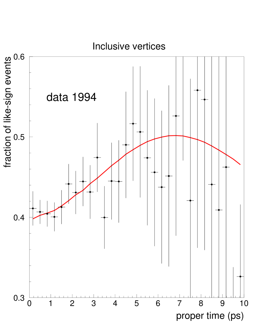
In Figures 9 and 10 the fractions of weighted - as described above - like-sign tagged
events, as a function
of the proper time, for the soft lepton sample and inclusive vertex sample,
are shown for
the 1992 to 2000 data. In these Figures, values of of 0.495 ps-1
and of 15 ps-1 are used in the parametrizations corresponding to the continuous lines.
Figure 9: Fraction of like-sign tagged events as a function of the reconstructed
proper time for the soft lepton and inclusive vertex samples.
The 1992 and 1993 data are shown as points with error bars, the parametrization is given as a solid line.Figure 10: Fraction of like-sign tagged events as a function of the
reconstructed proper time for the soft lepton and inclusive vertex samples. The 1994 to 2000 data are shown as points with error bars, the parametrization is given as a solid line.
2.7 Measurement of the oscillation frequency
The mass difference between the two physical states in the system was determined by fitting the fraction
of weighted like-sign tagged events - shown in Figures 9, 10 - as a function of the reconstructed proper time .
The following expression was used for the number of weighted like-sign events:
(25)
The total number of weighted events is equal to:
(26)
The event-by-event tagging purity is used as a weight.
The values for and for the B-hadron lifetimes were fixed at the values listed in
section 2.4.
is the total number of b quark events.
The functions and as well as the acceptance were parametrized using the simulation.
The total number of events from charm and uds quarks are obtained by intergrating these functions.
The tagging purities and
were taken from the simulation.
The like-sign tagged fraction was fitted in the range
from 0.5 to 12 ps using a binned fit. First a fit was performed on the simulated data, i.e.
the parametrization as shown in Figures 9 and 10. In this fit
, the mass difference, is fixed and
, , and are left free, where
is the tagging purity and
the tagging purity for the other b hadrons is parametrized as:
.
The parameter takes into account the slight dependence
of the tagging purity as a function of the proper time.
In a second fit, the data were fitted leaving free
, , and .
The parameter
was fixed to the value of obtained in the previous fit to the
simulation. The results for the different parameters are:
(0.579),
(0.554) and
(0.059). Within parentheses are given the results for the
fit to the simulated data.
The result for the mass difference is = 0.531
0.025 (stat.)
with a of 22.5/(23-4), as shown in Figure 11.
The reason for performing a four parameter fit is that both tagging purities
for
the meson and for the other B particles are determined using
the data. Therefore systematic
uncertainties on these parameters were largely reduced.
In this way the fit results become also less sensitive to, for example, the fraction of
mesons.
Due to the fact that the fit was first applied and tuned to the simulated data, the resolution function is taken into account.
Figure 11: Fraction of like-sign tagged events as a function of the reconstructed
proper time using
1992-2000 data. The data were shown as points with error bars, the solid line corresponds
to the fit.
A breakdown of the systematic errors affecting the measurement is given
in Table 6. The range of values for the fractions and lifetimes of
the different B species come from ref. [10].
The fractions of mesons and B baryons were
changed (correspondingly the other B fractions are recalculated) as
well as
the lifetimes and backgrounds.
The tagging correction factor (see section 2.6) was varied by a relative 5% for the soft lepton sample and by 15% for the inclusive vertex sample.
The proper times were scaled with 1%, coming from the scale uncertainty
on the reconstructed decay length and momentum, and the corresponding systematic
error on was -0.0049 ps-1.
The resolution function (see section 2.5) was smeared by an additional Gaussian term
with a width of 0.1+0.03 and the resulting shift in
was 0.0037 ps-1. This additional smearing corresponds to a 10% systematic error on the expected decay length resolution and a 10% systematic error on the expected momentum
resolution.
Table 6: The systematic errors affecting the measurement.
The final result is thus:
= (0.531 0.025 (stat) 0.007 (syst.)) ps-1.
The total error is therefore 0.027 ps-1.
This result for the
mass difference between the two physical states in the
system
is compatible with those from other experiments [10].
A fit was also performed to extract the width difference
.
In the fit, the expression in Eq. (25)
was replaced
by
and the expression in Eq. (26) was modified accordingly.
The result of the five parameter fit is .
The total systematic error was evaluated for the error sources listed in
Table 6 and found to be .
Using the measured lifetime [10],
.
The following upper limit was derived:
at 95% CL.
2.8 Search for oscillations
To search for oscillations a likelihood fit was performed,
where the negative log-likelihood is defined as:
(27)
where the expression for and can
be found in Eqs. (13) and (14).
To extract results from this fit the so-called amplitude method
was used [11]. For the mixed and unmixed events the following
expressions were used:
(28)
and similarly:
(29)
Bs oscillations will correspond to a value A of unity.
The oscillation amplitude and its error were fitted to the data as a function
of .
The result of the amplitude fit is shown in Figures 12 and 13.
Before discussing the result and its interpretation, the systematic errors
have been studied.
This was done by changing one parameter at a time (for example ) and
redoing the full amplitude fit.
The systematic error was then evaluated as [11]:
(30)
where () and () denote the fitted amplitude and error
before (after) changing the parameter. The last term in Eq.(30) takes into account the change in the error of the fitted amplitude.
The following parameters have been changed as in Table 6: from 0.097 to 0.108, the and charm backgrounds have been scaled up by 10%, the tagging purity has been changed by varying the correction factor by 5% for the soft
lepton tag and by 15% for the inclusive vertex tag, the constant term for , the width of the
resolution function (see section 2.5),
has been changed by a relative 10%, , the width of the resolution function for the
momentum, has been changed by a relative 10%.
The total systematic error as a function of is shown in
Figure 12b. It is at most 35% of the statistical error.
Using the results for the amplitude and its error it is
possible to obtain the 95% CL exclusion region or sensitivity. This region
corresponds to . This curve is shown in Figures 12
and 13.
No
oscillations have been
observed in the data.
A limit on the
mass difference of the two physical states can be put:
at 95 % CL.
Using the error on , , the sensitivity is found to be:
Sensitivity = 6.6 ps-1.
The sensitivity would be 6.8 ps-1 if the systematic error on
the amplitude was neglected666
In Table 7 the results are given for the amplitude and its error as a function of after adjusting to the recently published value of 0.106 [13]..
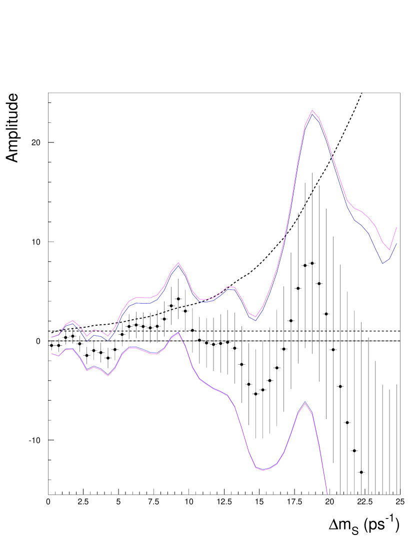
Figure 12: a) Fitted values of the oscillation amplitude as a function of . The horizontal line
corresponds to the value =1.
The black band is situated between the curves for
and .
b) The total amplitude
error as a function of .
The upper band is situated between the statistical error
()
and the total error ().
The lower curve shows the
systematic error .
The crossing point with the dashed line of the rising curve for the total error with =1/1.645 at
gives the sensitivity.Figure 13: Fitted values of the oscillation amplitude as a function of . The data are identical to those of Fig.12.
The dashed horizontal line
corresponds to =1.
The black band is situated between the curves for
and .
The smoothly rising curve corresponds to
.
The crossing point with =1 at
gives the expected lower limit at 95% CL.
(stat)
(total)
0.25
-0.17
0.11
0.13
0.75
0.12
0.15
0.17
1.25
0.46
0.18
0.20
1.75
0.35
0.21
0.23
2.25
0.13
0.23
0.26
2.75
0.16
0.25
0.28
3.25
0.19
0.28
0.31
3.75
0.26
0.31
0.33
4.25
0.23
0.34
0.37
4.75
0.13
0.37
0.40
5.25
0.39
0.41
0.43
5.75
0.65
0.45
0.47
6.25
0.30
0.50
0.53
6.75
-0.26
0.56
0.58
7.25
-0.53
0.62
0.65
7.75
-0.61
0.69
0.71
8.25
-0.71
0.76
0.78
8.75
-0.90
0.85
0.87
9.25
-1.02
0.95
0.96
9.75
-0.72
1.05
1.06
10.25
0.02
1.16
1.17
10.75
0.53
1.28
1.30
11.25
0.54
1.43
1.45
11.75
0.36
1.59
1.62
12.25
0.39
1.77
1.82
12.75
0.81
1.96
2.02
13.25
1.42
2.17
2.23
13.75
1.98
2.40
2.44
14.25
1.90
2.65
2.69
14.75
0.65
2.91
2.96
15.25
-1.11
3.17
3.22
15.75
-2.04
3.44
3.48
16.25
-1.36
3.74
3.84
16.75
0.88
4.08
4.30
17.25
3.90
4.45
4.77
17.75
6.61
4.85
5.14
18.25
8.43
5.27
5.44
18.75
9.36
5.69
5.79
19.25
9.66
6.12
6.23
19.75
8.99
6.53
6.68
20.25
8.22
6.92
7.09
20.75
8.00
7.33
7.47
21.25
8.02
7.79
7.93
21.75
8.63
8.31
8.52
22.25
10.32
8.89
9.19
22.75
12.47
9.48
9.84
23.25
14.58
10.05
10.43
23.75
16.20
10.62
11.03
24.25
17.11
11.21
11.68
24.75
17.77
11.82
12.38
Table 7: The amplitude and its statistical and systematic error as a function of after adjusting to the published value of 0.106 [13].
3 A neural network analysis
The inclusive analysis described in this section
was an attempt to optimize the statistical precision attainable in the high
region.
This analysis made extensive use of neural network techniques for tagging and
vertex reconstruction, mostly based on the BSAURUS [12] package.
Several neural networks were used on the event and track level.
For optimal performance a good resolution on the proper time was required
and this was achieved by keeping
the energy and the vertex reconstruction separated in the analysis.
The separated treatment of decay length and energy reconstruction led to a
CPU intensive two-dimensional integration for each event.
Only the best class of events (in terms of the decay length resolution) was
used, to reach an optimal performance for high values.
The restrictive cuts on quality and decay length resolution led to a sample
of only 30 k events for the data taken in 1994.
3.1 Event selection
Multihadronic Z0 events were selected requiring at least 5 reconstructed
tracks and a total reconstructed energy larger than 12% of the centre-of-mass energy.
The event was rejected if it had more than 3 jets or if
the value of was larger than 0.75.
The cosine of the opening angle between the two most energetic jets was required
to be less than .
Further, the value of the combined event b-tagging variable as
defined in ref. [5] had to be larger than .
Events having an identified lepton with a transverse momentum larger than 1.2
GeV/c were removed.
To obtain a homogeneous data set, it was required that both the
liquid and gas radiators of the Barrel RICH were fully operational.
The same selection was applied to simulated Z events using the JETSET 7.3 [6] generator.
Each event was split into hemispheres using the plane perpendicular to the
thrust axis. A first estimate of the B candidate momentum vector was
obtained by calculating the charged particles rapidities,
with respect to the thrust axis, and by summing the momenta of those with rapidity .
In each hemisphere a secondary vertex was fitted using the tracks with vertex detector hits from high rapidity
charged particles.
The secondary vertex fit was performed in three dimensions using as a constraint
the direction of the B candidate momentum vector.
The result of the vertex fit was used as an input to a Neural Network, the so-called TrackNet,
that distinguishes between a fragmentation track and a track originating from a weakly decaying B hadron.
In the final stage of the fit, the TrackNet output was used to add candidate tracks to the secondary vertex and the fit was redone.
Finally, a hemisphere was rejected if
the secondary vertex fit did not converge.
3.2 Flavour tagging
The tagging of the quark flavour at production and decay times is necessary to distinguish mixed from unmixed mesons.
Only the opposite hemisphere
was used for the production tag to reduce correlations between the production
and decay tags.
The decay tag was based on track-by-track flavour nets, which were later
combined using a likelihood ratio to tag the presence of a B or meson at decay time in each hemisphere. For the production tag a dedicated neural network was used.
3.3 The track-by-track flavour nets
Eight different networks were trained corresponding to a production and a
decay flavour network for each of the four B hadron types. The aim of each
network was to exploit, track-by-track, the correlation between the charge
of a single track and the b quark charge.
This approach is motivated by the different decay chains of the various types
of B hadrons where, for example, the ‘charge’ of the meson determines
the b quark charge.
The discriminating input variables are:
particle identification (e.g. kaon, proton and lepton probabilities),
B-D vertex separation based on a network trying to discriminate between
tracks originating from the weakly decaying B hadron and those from the
subsequent cascade meson decay, the momenta in the B rest frame and
variables related to tracking quality.
The track decay flavour nets use 21 input variables in total, while the track production flavour nets have
18 input variables; essentially the same input variables without the lepton
identification and the B-D net variables.
To obtain a flavour tag in a given hemisphere the individual track probabilities
( and production or decay) coming from the different networks were combined in the following way,
(31)
where is the charge. For the production flavour tag, tracks
with TrackNet values less than are selected, while for the decay flavour tag, tracks must have a TrackNet value above .
3.4 The production and decay flavour tag
The production flavour net was constructed using all the information available in the hemisphere, i.e.
the fragmentation and decay flavour probabilities ,
and the quality of the information for the selected hemisphere.
More details on the flavour networks and on the flavour tag can be found in [12].
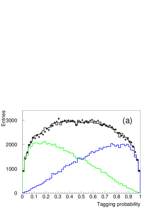
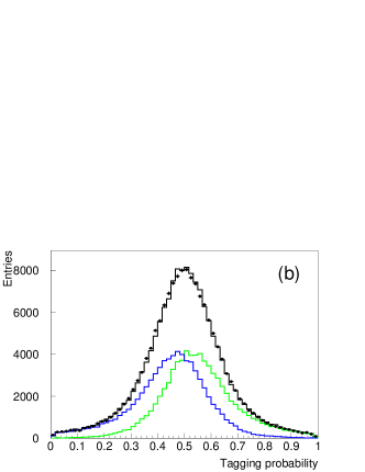
In Figure 14a the probability distribution for the production
tag for 1994 data and simulation is shown. The grey lines indicate the distributions for b and quarks. The achieved tagging purity on simulation is 71% at 100% efficiency.
For the decay flavour tag, the probability was used.
In Figure 14b the decay flavour probability distributions for 1994 data and simulation are shown.
The tagging purity on simulation was 62% at 100% efficiency.
The contributions from light and charm quarks are very small due to the high b purity of the sample of 98.3 %.
Figure 14: The
production (a) and decay (b) tag distributions for 1994 data and simulation.
The distributions for b and are indicated in light and dark grey. The decay tag
is optimized for and particles.
3.5 Energy reconstruction
To determine the proper time, a precise estimate of the energy of the
decaying B hadron is needed.
The starting point was a raw estimate of the B energy and mass
.
These quantities were determined by weighting (with a sigmoid threshold function) the momentum and energy
components of the charged particles by the TrackNet output value and the neutral particles
by their rapidity. For three-jet events only the rapidity was used as a weight.
In this way particles coming from the decaying B hadron receive a higher
weight.
The raw energy was corrected as a function of and of the fraction of the
energy in the hemisphere, , to obtain an improved estimate of
the energy.
This was done in the following way. The simulated data were divided
into several samples according to the measured ratio and
for each of these samples the , defined as the true energy minus the raw energy, was plotted as function of .
The median values of in each bin of were calculated and
the dependence was fitted by a third order polynomial:
(32)
The four parameters in each bin were then studied
as functions of and parametrized with third and
second-order polynomials.
In this way a smooth correction function was obtained.
This procedure led to an estimate of the B hadron energy.
Studies on simulated B events showed a large correlation between
the number of tracks and the B energy resolution.
For this reason, the number of tracks in the hemisphere was chosen to define
different resolution classes.
In total 16 different classes were defined, starting with 2 tracks per
hemisphere in class one and ending with 17 and more tracks in class 16.
The central Gaussian of a double Gaussian fit to the B energy resolution
varies from 4% in the best class to 15% in the worst.
3.6 Decay length reconstruction
Starting from the secondary vertex algorithm, described in section 3.1,
an optimized algorithm was developed with the aim of improving the decay
length resolution and of minimizing the forward bias resulting from the
inclusion of tracks from the cascade decay vertex in the B decay vertex
reconstruction.
Based on the output of the B-D net, a so-called ‘Stripping’ algorithm was
developed.
For the ‘Stripping’ algorithm candidate tracks were selected if they had
a TrackNet output larger than and a B-D net output value less than
.
The B-D net cut value corresponds to an efficiency of 50% for selecting a
track
from a weakly decaying B hadron at a purity of 75%.
A secondary vertex fit was performed if two or more tracks were selected.
If the fit failed to converge within the algorithm criteria and more than two tracks were selected, the track with highest contribution was
removed and the fit was repeated.
This procedure was done iteratively until convergence was reached or two tracks were left.
Finally, the direction of the B, as estimated by the B energy algorithm,
was used as a constraint.
The overall efficiency to find a vertex was about %.
Events with a very good decay length resolution were selected by requiring
that the expected error on the decay length was smaller than 200 .
Because of cuts on the TrackNet output, on the B-D output and on the expected
decay length
error,
less events will be reconstructed at small decay length.
Therefore an acceptance function depending on the true B decay length
was calculated using the simulation.
After having applied these cuts, 30k hemispheres were selected in the 1994
data sample. The b purity of the sample was estimated from simulated events
to be 98.3%.
3.7 The likelihood fit
In the fitting program, the like- and unlike-sign events were separated in the same way as described in section 2.5 of the previous analysis and the same expressions for like- and unlike-sign probabilities were used.
A difference from the previous analysis was the treatment of the resolution
functions and
, which were kept separated.
As a parameterization for the decay length two asymmetric Gaussian distributions were
chosen, while for the momentum reconstruction two symmetric Gaussian
distributions were used.
The probability for a B event to be observed at a proper time
is a convolution over an exponential B decay distribution,
an acceptance function , the true B hadron momentum distribution and the resolution functions and , all four taken from simulation:
(33)
were denotes the B lifetime and Eq. (8) was used to calculate the proper time.
3.8 Modelling simulation and data
As explained in section 2.6 it is important to model
precisely the tagging purities.
In this analysis the raw purities were modified using
a parameter as defined in Eq. (17).
The decay and production tag parameters for the different particles were obtained
from simulation, and are listed in Table 8.
particle
decay tag
particle
production tag
1
b quarks
0.94
1.08
c quarks
0.56
1.15
uds quarks
0.84
0.93
c quarks
1.05
uds quarks
0.08
Table 8: The parameters for the decay and production tag for the different particles as obtained from the 1994 simulation
For the real data, the correction factor , defined
in Eq. (19), was determined from the fraction of like-sign events, using the same method as was discussed in section 2.6.
Two correction factors were needed, one for mesons and one for
the other B mesons.
Their values were and .
Using the amplitude method [11] the result shown in Figure
15a was obtained. A limit on was not extracted as the
analysis was optimized for high values of .
Figure 15b shows the agreement between the data and the
description by the fitting programme.
Figure 15: In the left plot the
fitted oscillation amplitude for the NN analysis is shown
as a function of
as
points and error bars. The continuous (dotted) lines correspond to . The dashed line corresponds to .
The plot on the right side shows the fraction of weighted like-sign tagged events as a function of the
proper time. The data are shown as points with error bars, the parametrization
is given as a solid line.
Systematic uncertainties have been evaluated by varying a single parameter at a
time
(e.g ) and redoing the full amplitude fit. The systematic error was
then calculated as defined in Eq. (30).
The same parameters as described in section 2.8 were varied
and the systematic error
was determined to be at most 25% of the statistical error.
The error on the fitted amplitude at of 15 and 20 ps-1 gives respectively
5.1 and 11.8 for this analysis
using only 1994 data. This can be compared with the
values of
5.0 and 10.9 obtained with the previous analysis using only the 1994 data sample.
The results of the neural network analysis optimized
for high values of are compatible with
the results for the 1992-2000 data
shown in section 2.8. No attempt is made to combine the results.
4 Conclusion
Using a total sample of 770 k events - of which 155 k events contain a soft lepton - the mass difference
between the two physical states in the
system
was measured to be:
.
The following limit on the width difference between the two states was obtained:
at 95% CL.
As no evidence for
oscillations was found, a limit on the
mass difference of the two physical states was given:
at 95 % CL
with a sensitivity equal to 6.6 ps-1.
These results are compatible with a neural network analysis
optimized for high values of .
Acknowledgements
We are greatly indebted to our technical
collaborators, to the members of the CERN-SL Division for the excellent
performance of the LEP collider, and to the funding agencies for their
support in building and operating the DELPHI detector. We acknowledge in particular the support of Austrian Federal Ministry of Education, Science and Culture,
GZ 616.364/2-III/2a/98, FNRS–FWO, Flanders Institute to encourage scientific and technological
research in the industry (IWT), Belgium, FINEP, CNPq, CAPES, FUJB and FAPERJ, Brazil, Czech Ministry of Industry and Trade, GA CR 202/99/1362, Commission of the European Communities (DG XII), Direction des Sciences de la Matire, CEA, France, Bundesministerium fr Bildung, Wissenschaft, Forschung
und Technologie, Germany, General Secretariat for Research and Technology, Greece, National Science Foundation (NWO) and Foundation for Research on Matter (FOM),
The Netherlands, Norwegian Research Council, State Committee for Scientific Research, Poland, SPUB-M/CERN/PO3/DZ296/2000,
SPUB-M/CERN/PO3/DZ297/2000, 2P03B 104 19 and 2P03B 69 23(2002-2004) JNICT–Junta Nacional de Investigação Científica
e Tecnolgica, Portugal, Vedecka grantova agentura MS SR, Slovakia, Nr. 95/5195/134, Ministry of Science and Technology of the Republic of Slovenia, CICYT, Spain, AEN99-0950 and AEN99-0761, The Swedish Natural Science Research Council, Particle Physics and Astronomy Research Council, UK, Department of Energy, USA, DE-FG02-01ER41155.
References
[1] G. Altarelli and P.J. Franzini, Zeit. Phys C37 (1988) 271. P.J. Franzini, Phys. Rep. 173 (1989) 1.
[2]
M. Ciuchini et al., JHEP 0107:013, 2001 hep-ph/0012308.
[3] L. Wolfenstein, Phys. Rev Lett. 51 (1983) 1945.
[4]
DELPHI Coll., P. Abreu et al., Eur. Phys. J C18 (2000) 229, DELPHI Coll., P. Abreu et al., Eur. Phys. J. C16 (2000) 555, DELPHI Coll., P. Abreu et al., Phys. Lett. B414 (1997) 382.
[5] G. V. Borisov and C. Mariotti, Nucl. Instr. and Meth. A372 (1996) 181, G. V. Borisov Combined b-tagging, DELPHI Note, PHYS 716-94 (1997).
[6] T. Sjöstrand, PYTHIA 5.7 and JETSET 7.4, Computer Physics
Commun. 82 (1994) 74.
[7] DELPHI Coll., P. Aarnio et al., Nucl. Inst. Meth.
A303 (1991) 233, DELPHI Coll., P. Abreu et al., Nucl. Inst. Meth. A378 (1996) 57.
[8] DELPHI Coll., P. Abreu et al, Zeit. Phys.
C71 (1996) 11.