Measurements of the Branching Fractions of Charged $B$ Decays to $K^{+}\pi^{-}\pi^{+}$ Final States

The BABAR Collaboration

Abstract

We present preliminary results of searches for exclusive charged–$B$ decays to $K^{\pm}\pi^{\mp}\pi^{\pm}$ from 61.6 million $B\kern 1.79993pt\overline{\kern-1.79993ptB}{}$ pairs collected at the ${\mathchar 28935\relax\rm(4S)}$ resonance with the BABAR detector at the SLAC PEP-II asymmetric $B$ Factory. The Dalitz plot is divided into eight regions and, using a maximum–likelihood fit, we measure statistically significant yields in all regions. We interpret the results as the following branching fractions averaged over charged–conjugate states: $\mbox{${\cal B}$}(\mbox{$B^{+}\rightarrow\mbox{$K^{*0}(892)\pi^{+}$}$},K^{*0}\rightarrow K^{+}\pi^{-})=(10.3\pm 1.2^{+1.0}_{-2.7})\times 10^{-6}$, $\mbox{${\cal B}$}(\mbox{$B^{+}\rightarrow\mbox{$\mbox{$f_{0}(980)$}K^{+}$}$},f_{0}\rightarrow\pi^{+}\pi^{-})=(9.2\pm 1.2^{+2.1}_{-2.6})\times 10^{-6}$, $\mbox{${\cal B}$}(\mbox{$B^{+}\rightarrow\mbox{$\chi_{c0}K^{+}$}$},\chi_{c0}\rightarrow\pi^{+}\pi^{-})=(1.46\pm 0.35\pm 0.12)\times 10^{-6}$ and $\mbox{${\cal B}$}(\mbox{$B^{+}\rightarrow\mbox{$\kern 1.99997pt\overline{\kern-1.99997ptD}{}^{0}\pi^{+}$}$},\kern 1.99997pt\overline{\kern-1.99997ptD}{}^{0}\rightarrow K^{+}\pi^{-})=(184.6\pm 3.2\pm 9.7)\times 10^{-6}$. The first uncertainty is statistical and the second is systematic and includes resonance–model and interference uncertainties. We give 90% confidence-level upper limits on the branching fractions of the following channels: $\mbox{${\cal B}$}(\mbox{$B^{+}\rightarrow\mbox{$\rho^{0}(770)K^{+}$}$})<6.2\times 10^{-6}$ and $\mbox{${\cal B}$}(B^{+}\rightarrow K^{+}\pi^{-}\pi^{+}$ non–resonant) $<17\times 10^{-6}$.

1 Introduction

The study of charmless hadronic $B$ decays can make important contributions to the understanding of $C\!P$ violation in the Standard Model as well as to models of hadronic decays. The measurement of $B^{+}$ decays to the final state $K^{+}\pi^{-}\pi^{+}$ via intermediate resonances can be used to search for direct $C\!P$ violation. The three–body final state is unique in the search for weak phases since it is possible to isolate the strong phase variation for overlapping resonances. There has been recent theoretical progress on proposed methods for extracting the Cabibbo–Kobayashi–Maskawa angle $\gamma$ through the interference of $\chi_{c0}K^{+}$ with other $K^{+}\pi^{-}\pi^{+}$ final states [1, 2]. Study of these decays can also help clarify the nature of the resonances involved, not all of which are well understood. We present preliminary results on the branching fractions of $B^{+}$ decays to the final state $K^{+}\pi^{-}\pi^{+}$ both non–resonant and by way of intermediate resonances.

2 The BABAR Detector and Dataset

The data used in this analysis were collected with the BABAR detector at the PEP-II asymmetric–energy $e^{+}e^{-}$ storage ring at SLAC. The data sample consists of 61.6 million $B\kern 1.79993pt\overline{\kern-1.79993ptB}{}$ pairs, corresponding to an integrated luminosity of 56.4 $\mbox{\,fb}^{-1}$ collected on the ${\mathchar 28935\relax\rm(4S)}$ resonance (10.58 $\mathrm{\,Ge\kern-1.00006ptV}$) during the 2000-2001 run. In addition, a total integrated luminosity of 6.4 $\mbox{\,fb}^{-1}$ was taken 40 $\mathrm{\,Me\kern-1.00006ptV}$ below the ${\mathchar 28935\relax\rm(4S)}$ resonance, and was used to study backgrounds from continuum production.

The BABAR detector is described in detail elsewhere [3]; the main parts relevant for this analysis are the tracking and particle identification sub–systems.

The 5–layer double–sided silicon vertex tracker (SVT) measures the impact parameters, angles, and transverse momenta of tracks. Outside the SVT is a 40–layer drift chamber (DCH), which measures the transverse momenta of tracks from their curvature in the 1.5-T solenoidal magnetic field. The ionization energy loss of charged tracks, $\mathrm{d}E/\mathrm{d}x$, in the SVT and DCH is used in the particle–type identification. The tracking system has a momentum resolution of 0.5% for a transverse momentum of 1.0 ${\mathrm{\,Ge\kern-1.00006ptV\!/}c}$ and a typical $\mathrm{d}E/\mathrm{d}x$ resolution of $7.5$%.

Surrounding the DCH is a detector of internally–reflected Cherenkov radiation (DIRC), which provides charged–hadron identification in the barrel region. The separation between pions and kaons varies from $>8\sigma$ at 2.0${\mathrm{\,Ge\kern-1.00006ptV\!/}c}$ to 2.5$\sigma$ at 4.0${\mathrm{\,Ge\kern-1.00006ptV\!/}c}$, where $\sigma$ is the average resolution on the Cherenkov angle.

The DIRC is surrounded by a Cesium Iodide electromagnetic calorimeter (EMC), which is used to measure the energies and angular positions of photons and electrons with excellent resolution. In this analysis, the EMC is used to veto electrons.

3 Analysis Method

The $K^{+}\pi^{-}\pi^{+}$ final state can be represented in a Dalitz plot [4]. The many resonant $B$ decay modes form bands in such a plot. These resonances often overlap and interfere so the whole Dalitz plot should be considered before assigning a branching fraction to a specific mode. This analysis divides the Dalitz plot into regions, each of which is expected to be dominated by a particular contribution. First the yields in these regions are determined, using a maximum–likelihood fit, with no assumption on the form of the intermediate resonances. We then interpret these yields as branching fractions, assuming a model for the contributions to the Dalitz plot. We also consider the uncertainty of the model and the effect of overlap and interference between these contributions.

3.1 Dalitz Plot Regions

The $K^{+}\pi^{-}\pi^{+}$ Dalitz plot is divided into eight regions. Each region is designed to contain a large proportion of the decays of the expected dominant resonance (if any) and to minimize contributions from neighboring modes. The definitions of the regions are given in Table 1 and they are illustrated in Figure 1.

Regions I, II and III are characterized by narrow bands in the invariant mass of the $K^{+}\pi^{-}$ system, $m_{K\pi}$. Region I is expected to be dominated by the $K^{*0}(892)$. The primary resonance contribution to region II, labeled “higher $K^{*0}$”, is not currently known. The areas where these bands cross the $\pi\pi$ resonances ($\rho(770),\mbox{$f_{0}(980)$}$, “higher $f$” and $\chi_{c0}$) are excluded to limit biases from interference. Region III is dominated by the production of $\kern 1.99997pt\overline{\kern-1.99997ptD}{}^{0}\pi^{+}$. The relatively high branching fraction for this mode allows it to be used to correct for differences between data and simulated events and evaluate systematic uncertainties.

Regions IV, V and VI are characterized by narrow bands in the $\pi^{+}\pi^{-}$ invariant mass, $m_{\pi\pi}$. Regions IV and V are expected to be dominated by the $\rho(770)$ and $f_{0}(980)$, respectively. The resonance contributions to region VI (“higher $f$”) are not well defined. The area where these regions would intersect the $\kern 1.99997pt\overline{\kern-1.99997ptD}{}^{0}$ band, $1.8<m_{K\pi}<1.9{\mathrm{\,Ge\kern-1.00006ptV\!/}c^{2}}$, is excluded from regions IV, V and VI. The area where the other $K\pi$ resonances cross is not excluded from regions IV, V and VI as the overall interference uncertainty on $\mbox{${\cal B}$}(\mbox{$B^{+}\rightarrow\mbox{$\mbox{$f_{0}(980)$}K^{+}$}$})$ and $\mbox{${\cal B}$}(\mbox{$B^{+}\rightarrow\mbox{$\rho^{0}(770)K^{+}$}$})$ was estimated to be smaller when this area is excluded. Region VII, denoted “high mass”, could contain higher charmless and charmonium resonances as well as a non–resonant contribution.

Region VIII is dominated by $\chi_{c0}K^{+}$. A lower limit on $m_{K\pi}$ ensures that this region is free of contamination from resonances in regions I, II and III. The area $3.355<m_{\pi\pi}<3.475{\mathrm{\,Ge\kern-1.00006ptV\!/}c^{2}}$ is removed from all other regions to avoid this charmonium background.

Table 1: Regions of the $K^{+}\pi^{-}\pi^{+}$ Dalitz plot. The regions are kinematically defined by the $m_{K\pi}$ and $m_{\pi\pi}$ mass selection criteria. The symbol “$!$” is used to imply exclusion. The assumed dominant contribution is noted for each region.

Region	Dominant	Selection Criteria
	Contribution	$m_{K\pi}$ (${\mathrm{\,Ge\kern-1.00006ptV\!/}c^{2}}$)	$m_{\pi\pi}$ (${\mathrm{\,Ge\kern-1.00006ptV\!/}c^{2}}$)
I	$K^{*0}(892)\pi^{+}$	$0.816<m_{K\pi}<0.976$	$m_{\pi\pi}>1.5$  $!(3.355<m_{\pi\pi}<3.475)$
II	“higher $K^{*0}$” $\pi^{+}$	$0.976<m_{K\pi}<1.8$	$m_{\pi\pi}>1.5$  $!(3.355<m_{\pi\pi}<3.475)$
III	$\kern 1.99997pt\overline{\kern-1.99997ptD}{}^{0}\pi^{+}$	$1.835<m_{K\pi}<1.895$	$!(3.355<m_{\pi\pi}<3.475)$
IV	$\rho^{0}(770)K^{+}$	$!(1.8<m_{K\pi}<1.9)$	$0.6<m_{\pi\pi}<0.9$
V	$\mbox{$f_{0}(980)$}K^{+}$	$!(1.8<m_{K\pi}<1.9)$	$0.9<m_{\pi\pi}<1.1$
VI	“higher $f$” $K^{+}$	$!(1.8<m_{K\pi}<1.9)$	$1.1<m_{\pi\pi}<1.5$
VII	“high mass”	$m_{K\pi}>1.9$	$m_{\pi\pi}>1.5$  $!(3.355<m_{\pi\pi}<3.475)$
VIII	$\chi_{c0}K^{+}$	$m_{K\pi}>1.9$	$3.37<m_{\pi\pi}<3.46$

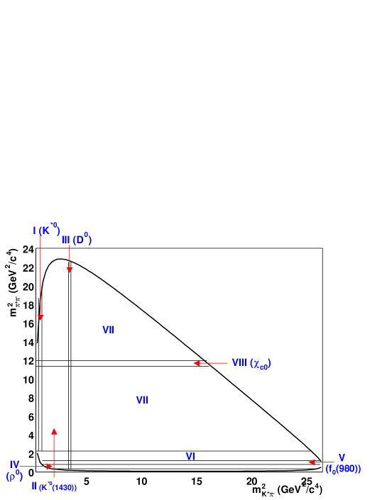
Figure 1: An illustration of the different regions in the Dalitz plot as defined in Table 1.

3.2 Candidate Selection

$B$ candidates are reconstructed from charged tracks that have at least 12 hits in the DCH, a maximum momentum of 10 ${\mathrm{\,Ge\kern-1.00006ptV\!/}c}$, a minimum transverse momentum of 100 ${\mathrm{\,Me\kern-1.00006ptV\!/}c}$, and originate from the beam–spot. The $B$ candidates are formed from three–charged–track combinations and particle identification selections are applied. Mass hypotheses are assigned accordingly and the $B$ candidates’ energies and momenta are required to satisfy appropriate kinematic constraints.

Two kinematic variables are defined that are included in the maximum–likelihood fit described later. The first of these is the beam–energy–substituted mass $\mbox{$m_{\rm ES}$}=\sqrt{(E^{2}_{b}-{\bf p}^{2}_{B})}$. The energy of the $B$ candidate is defined as $E_{b}=(\mbox{${1\over 2}$}s+{\bf p}_{0}\cdot{\bf p}_{B})/E_{0}$, where $\sqrt{s}$ and $E_{0}$ are the total energies of the $e^{+}e^{-}$ system in the center–of–mass (CM) and laboratory frames, respectively, and ${\bf p}_{0}$ and ${\bf p}_{B}$ are the three–momenta in the laboratory frame of the $e^{+}e^{-}$ system and the $B$ candidate, respectively. The $m_{\rm ES}$ value should be close to the nominal $B$ mass for signal events.

The second variable used is the energy difference, $\Delta E$, between the energy in the CM of the reconstructed $B$ candidate, $E_{B}^{*}$, and the beam energy, $\Delta E=E_{B}^{*}-\sqrt{s}/2$. $\Delta E$ is dependent on the mass hypotheses of the tracks. To each track a mass is assigned appropriate for the particle identification selections applied. For signal events, $\Delta E$ should be centered at zero.

To identify charged pions and kaons, we use $\mathrm{d}E/\mathrm{d}x$ information from the SVT and DCH for tracks with momenta below 700 ${\mathrm{\,Me\kern-1.00006ptV\!/}c}$, the number of photons measured by the DIRC for tracks with momenta above 500 ${\mathrm{\,Me\kern-1.00006ptV\!/}c}$, and the Cherenkov angle for tracks with momenta above 700 ${\mathrm{\,Me\kern-1.00006ptV\!/}c}$. Kaons are selected with requirements on the product of likelihood ratios determined from these measurements and pions are required to fail the kaon selection. The average selection efficiency for kaons in our final state that have passed the tracking requirements is $\sim 80\%$ including geometrical acceptance, while the misidentification probability of pions as kaons is below 5% at all momenta. The kaon veto on pions in our final state is $\sim 98\%$ efficient. We veto electron candidates by requiring that they fail a selection based on information from $\mathrm{d}E/\mathrm{d}x$, shower shapes in the EMC and the ratio of the shower energy and track momentum. The probability of misidentifying electrons as pions is approximately 5%, while the probability of misidentifying pions as electrons is $\sim 0.2\%$.

3.3 Background Suppression and Characterization

The dominant background in this analysis is from light quark and charm continuum production. This background is suppressed by imposing requirements on topological event shape variables, and the remainder is characterized and parameterized in the maximum–likelihood fits used to extract the signal yield from the data. There are also backgrounds from $B$ decays which, although contributing far fewer events, can be more difficult to separate from the signal and must also be parameterized in the fit, which is described in detail later.

The event shape variables used to suppress continuum background are calculated in the ${\mathchar 28935\relax\rm(4S)}$ rest frame. The first is the cosine of the angle $\theta_{T}$ between the thrust axis of the selected $B$ candidate and the thrust axis of the rest of the event, i.e., of all charged tracks and neutral particles not in the $B$ meson candidate. For continuum backgrounds, the directions of the two axes tend to be aligned because the daughters of the reconstructed candidate generally lie along the dijet axis of such events so the distribution of $\cos\theta_{T}$ is strongly peaked towards $\pm 1$. For $B$ events, however, the distribution is isotropic because the decay products from the two $B$ mesons are independent of each other and the $B$  mesons have very low momenta in the ${\mathchar 28935\relax\rm(4S)}$ rest frame. To improve the signal–to–background ratio, the criterion $|\cos\theta_{T}|<0.9$ is applied to all regions except region III ($\kern 1.99997pt\overline{\kern-1.99997ptD}{}^{0}$). This selection removes about 60% of the continuum background while retaining over 90% of the signal. The $\cos\theta_{T}$ requirement in the $\kern 1.99997pt\overline{\kern-1.99997ptD}{}^{0}$ region is varied to estimate a systematic uncertainty on the efficiency of this criterion in the other regions.

We also make use of a Fisher discriminant [5], using a linear combination of the angle between the $B$ candidate momentum and the beam direction; the angle between the $B$ candidate thrust axis and the beam direction; and the energy flow of the rest of the event into each of 9 independent concentric $10^{\circ}$ cones around the thrust axis of the reconstructed $B$ [6]. The variables and weights of the Fisher discriminant were chosen to optimize the separation of our final state and the continuum background after the $\cos\theta_{T}$ criterion has been applied. The resulting Fisher variable, ${\cal{F}}$, is used in the maximum–likelihood fit.

The $B$ decay backgrounds are from four main sources: combinatorial background from three unrelated tracks; three– and four-body $B\rightarrow D$ decays; charmless four–body decays with a missing track and three–body decays with one or more particles misidentified. These backgrounds are reduced by the particle identification selections and, where possible, removed by vetoing regions of the invariant–mass spectra of pairs of the final–state particles. The influence of remaining specific backgrounds on the signal yield obtained from the maximum–likelihood fit was established using test fits with Monte–Carlo simulated data (MC) with the expected number of signal, continuum background and $B$ background events. Background modes that significantly contributed to the signal yields in these tests are parameterized for the final fit to the data. However, if the background contributes only a few events, it is instead subtracted from the signal yield.

The combinatorial background from $B$ decays is less than 2% of the continuum background. The shape of its $\Delta E$ and $m_{\rm ES}$ distributions are similar to the continuum background and these events were found to be fitted as such in the test fits so no additional parameterisation was required.

The particle–misidentification background has several sources. $B^{+}\rightarrow{J\mskip-3.0mu/\mskip-2.0mu\psi\mskip 2.0mu}K^{+}$ and $B^{+}\rightarrow\Psi(2S)K^{+}$ decays which contribute through muon/pion misidentification are removed completely by excluding events with $2.97<m_{\pi\pi}<3.17{\mathrm{\,Ge\kern-1.00006ptV\!/}c^{2}}$ or $3.56<m_{\pi\pi}<3.76{\mathrm{\,Ge\kern-1.00006ptV\!/}c^{2}}$. This also excludes other $B$ backgrounds containing ${J\mskip-3.0mu/\mskip-2.0mu\psi\mskip 2.0mu}$ or $\Psi(2S)$, such as $B^{+}\rightarrow{J\mskip-3.0mu/\mskip-2.0mu\psi\mskip 2.0mu}K^{*+}$. The contributions from $B^{+}\rightarrow K^{+}e^{+}e^{-}$ are negligible due to the electron veto. Non–resonant $B^{+}\rightarrow K^{+}\mu^{+}\mu^{-}$ decays contribute with $18\pm 7$ events uniformly distributed over the Dalitz plot, using the branching fraction from [7]. Events are expected only in regions II, VI and VII where they are subtracted from the yields. Contributions from the $B^{+}\rightarrow\pi^{+}\pi^{-}\pi^{+}$ and $B^{+}\rightarrow K^{+}K^{-}\pi^{+}$ final states may affect regions I, II, IV, VI and VII. The channels concerned have not yet been observed and so an additional negative uncertainty is added to the signal yield equal to the number of events expected in the fit corresponding to the upper limit measured in [8]. This is 20 events for region VII and 6 events or fewer for all other regions.

The decay $\mbox{$B^{+}\rightarrow\mbox{$\kern 1.99997pt\overline{\kern-1.99997ptD}{}^{0}\pi^{+}$}$},\kern 1.99997pt\overline{\kern-1.99997ptD}{}^{0}\rightarrow K^{+}\pi^{-}\pi^{0}$ contributes to the measured signal yield when not parameterized in the test fits in regions II and VII, while $B^{+}\rightarrow\kern 1.99997pt\overline{\kern-1.99997ptD}{}^{0}\rho^{+}(770)$ with $\kern 1.99997pt\overline{\kern-1.99997ptD}{}^{0}\rightarrow K^{+}\pi^{-}$ and $\rho^{+}\rightarrow\pi^{+}\pi^{0}$ has a significant effect on the test fits in region VII. These modes are therefore parameterized in the final fit for the affected regions.

The decay $B^{+}\rightarrow\eta^{\prime}K^{+}$ with $\eta^{\prime}\rightarrow\rho^{0}(770)\gamma$, $\rho^{0}\rightarrow\pi^{+}\pi^{-}$ is the only charmless channel with a four–body final state found to contribute significantly. The expected number of events is 31 and 12 in regions IV and V, respectively, using the branching ratio measured in [9]. If not parameterized, these contribute to the signal yields in the test fits. This mode is therefore included in the final fit for those regions.

3.4 The Maximum–Likelihood Fit

We form Probability Density Functions (PDFs) for the 3 variables $m_{\rm ES}$, $\Delta E$ and $\mathcal{F}$ in each region. For each hypothesis $l$ (signal, continuum background, and if applicable, $B$ background) these three PDFs form a product $P_{l}$, which models that particular hypothesis. These products are functions of the variables $\vec{x}$ and parameters $\vec{\alpha}$ of the PDFs. The likelihood for an event $j$ is formed by summing the products over the $M$ hypotheses, with each product weighted by the number of events in that hypothesis $n_{l}$. A product over the $N$ events in the data sample of the per–event likelihoods along with a Poisson factor forms the total likelihood function $\mathcal{L}$, written in equation (1).

$$\mbox{$\mathcal{L}$}\,=\,\exp\left(-\sum_{i=1}^{M}n_{i}\right)\,\prod_{j=1}^{N}\,\left(\sum_{l=1}^{M}n_{l}\,P_{l}(\vec{\alpha},\vec{x_{j}})\right).$$ (1)

The fit is performed in two stages for each region. First, one–dimensional fits are performed on the particular data samples detailed below in order to determine the PDF parameters. Then the multivariate fit is performed on the final data samples to extract the signal and continuum background yields.

The signal PDF parameters, particularly the width of the $\Delta E$ distribution, vary across the Dalitz plane. Therefore, they are found for each region separately using Monte–Carlo–simulated signal of the expected dominant resonance where available and, otherwise, non–resonant $K^{+}\pi^{-}\pi^{+}$ selected for that region. Some differences have been observed between MC and data in the distributions of the $m_{\rm ES}$, $\Delta E$ and $\mathcal{F}$ variables. These differences are measured in the high–statistics $B^{+}\rightarrow\kern 1.99997pt\overline{\kern-1.99997ptD}{}^{0}\pi^{+}$ dominated region and are used to correct all regions where all the signal PDF parameters are fixed in the final fits. The $m_{\rm ES}$ PDF is a Crystal Ball function[10], the $\Delta E$ PDF is two Gaussians with equal means and the $\cal{F}$ PDF is a “bifurcated” Gaussian (a Gaussian with different widths above and below the mean).

The background PDF parameters are also found to vary across the Dalitz plane and so are determined individually for each region. The $\cal{F}$ PDF is a bifurcated Gaussian where the parameters are determined using data sidebands defined by $0.1<|\Delta E|<0.35\mathrm{\,Ge\kern-1.00006ptV}$ except in regions II and VII where, due to $B$ background, only the positive $\Delta E$ sideband is used. The $m_{\rm ES}$ variable is parameterized by the Argus threshold function [11] with two parameters: a fixed kinematic endpoint and a shape parameter which is left to float in the final fits. The $\Delta E$ PDF is a first–order polynomial where the gradient is also left to float in the final fits.

4 Physics Results

4.1 Fit Results

The signal yields for the various regions of the $K^{+}\pi^{-}\pi^{+}$ Dalitz plot are shown in Table 2. The first uncertainty is statistical and the second is systematic. The systematic uncertainty is from the uncertainties on the PDF parameters and from the $B$ background subtraction. The yields are found to be statistically significant in all regions ($>5\sigma$), where the statistical significance is taken as $\sqrt{-2\log(\mathcal{L}_{max}/\mathcal{L}_{(n_{sig}=0)})}$.

Table 2: Signal yields for the regions of the Dalitz plot before and after $B$ background subtraction. The first uncertainty is statistical, the second systematic.

Region	Signal Yield	Signal Yield after $B$
		background subtraction
I	$161\pm 18\pm 4$	$161\pm 18\pm 4$
II	$406\pm 28\pm 12$	$405\pm 28^{+12}_{-13}$
III	$3755\pm 66\pm 11$	$3755\pm 66\pm 11$
IV	$66\pm 15\pm 3$	$66\pm 15^{+3}_{-7}$
V	$179\pm 19\pm 5$	$179\pm 19\pm 5$
VI	$127\pm 19\pm 5$	$126\pm 19\pm 5$
VII	$147\pm 23\pm 7$	$133\pm 23^{+9}_{-22}$
VIII	$26\pm 6\pm 1$	$26\pm 6\pm 1$

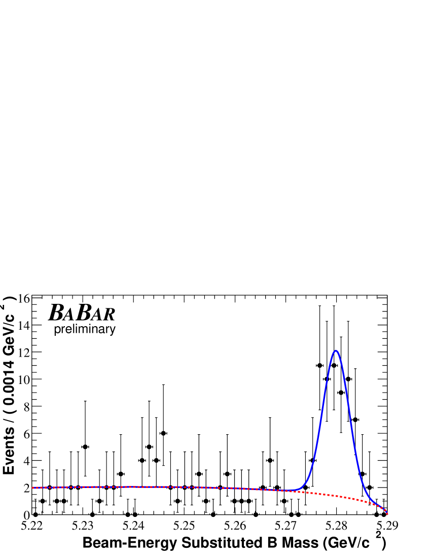
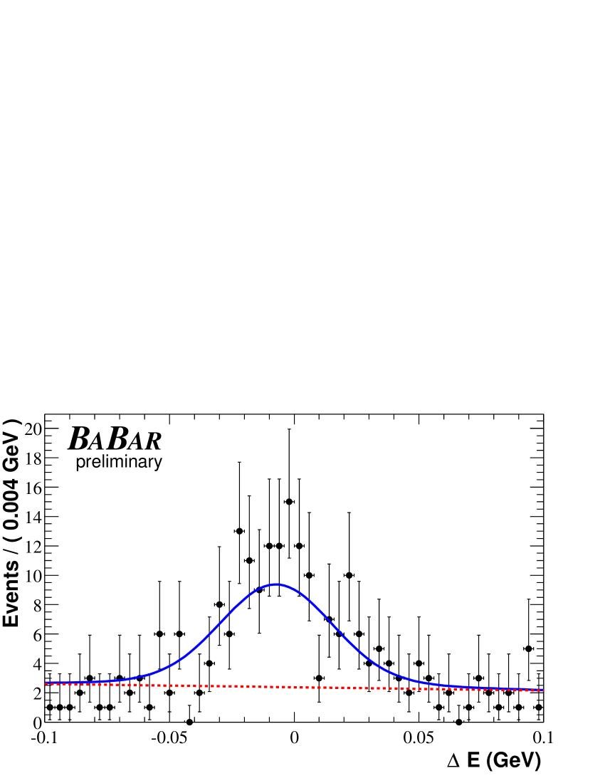
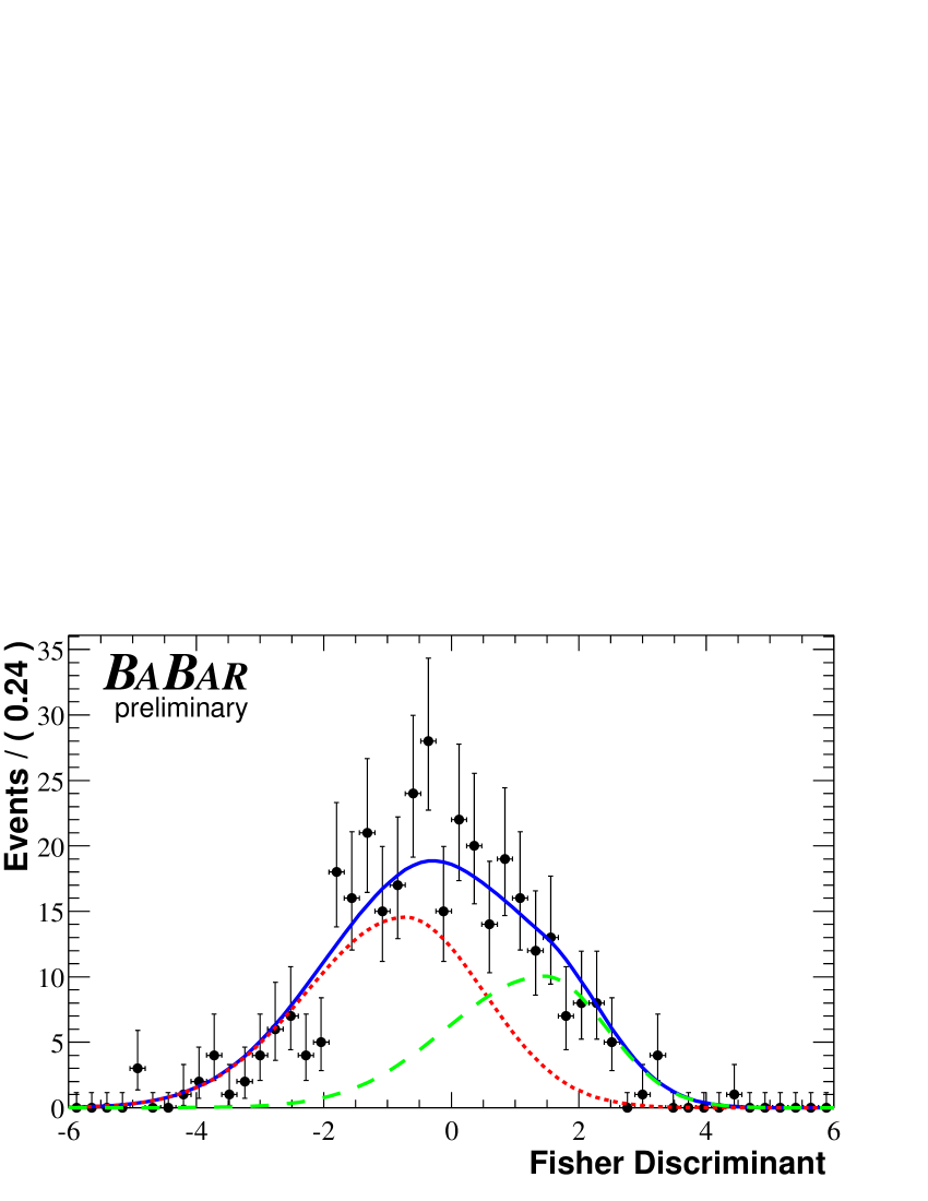
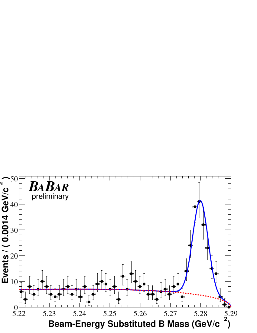
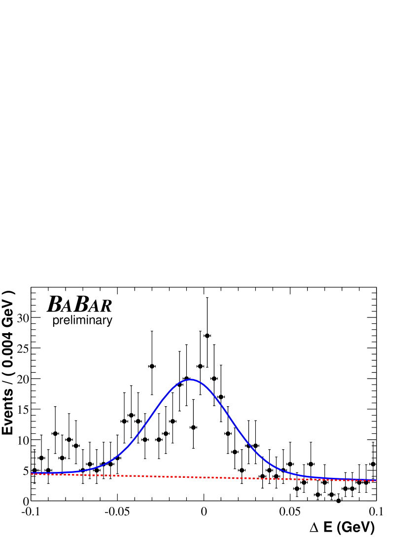
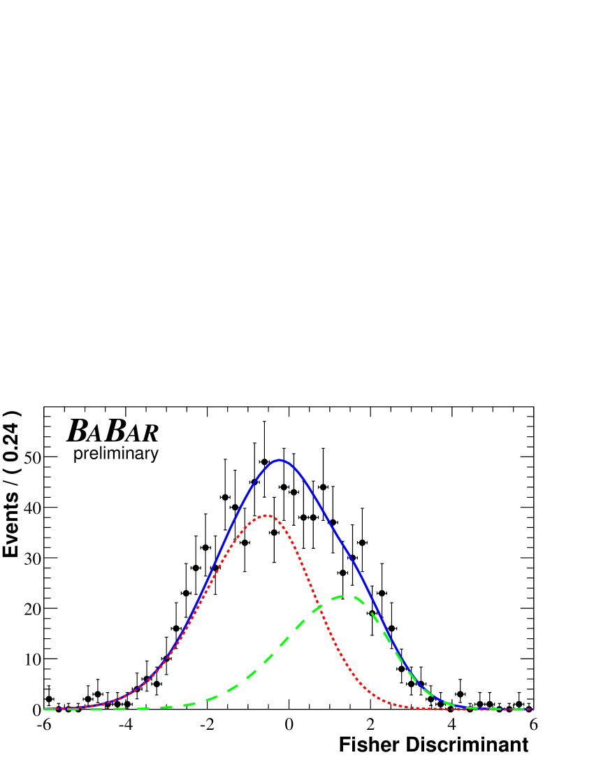
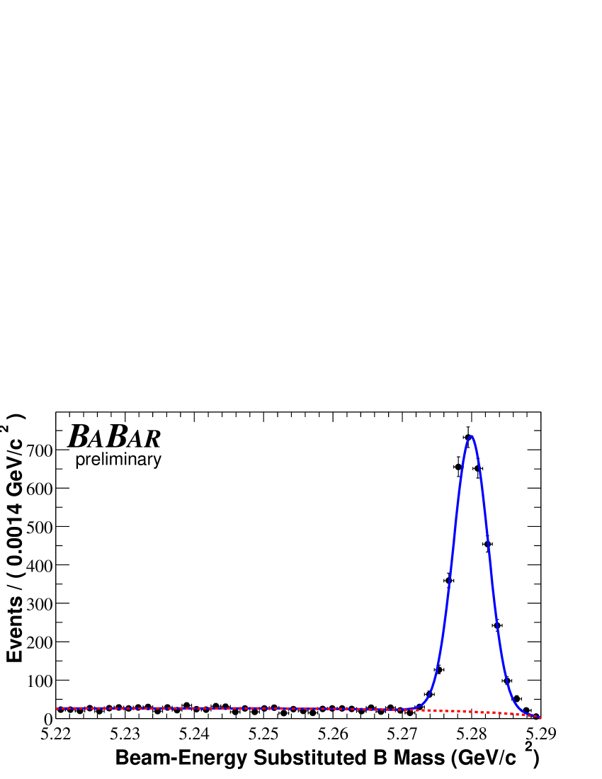
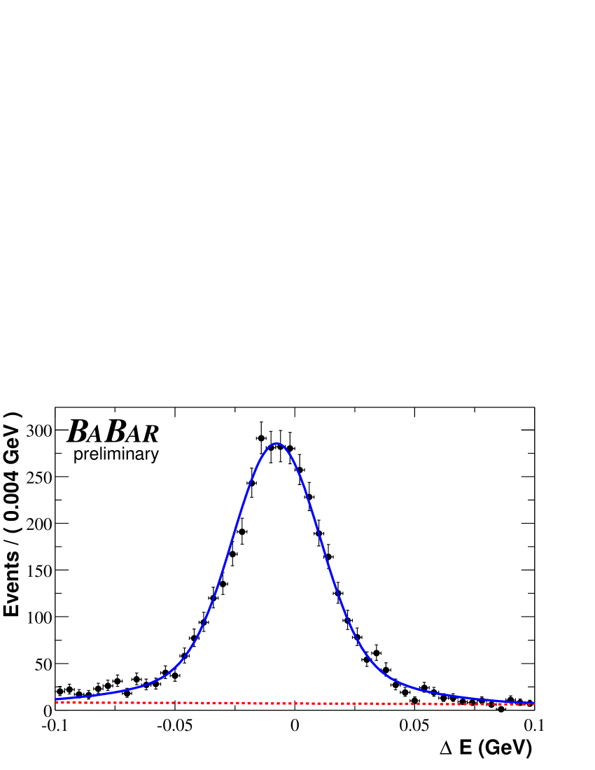
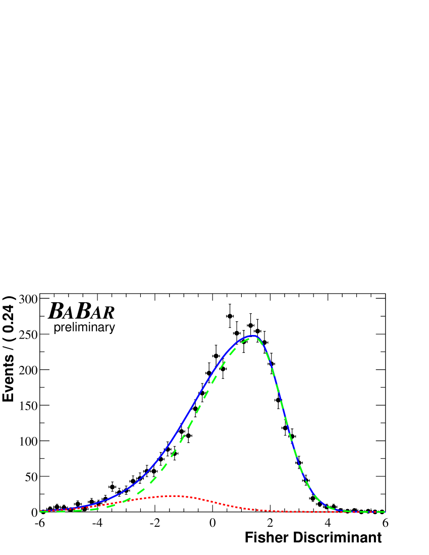
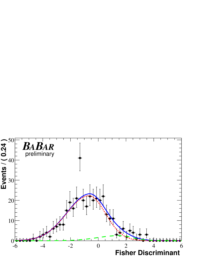
Figure 2: Projection plots in $m_{\rm ES}$, $\Delta E$ and ${\cal F}$, produced by selecting on the event likelihood ratio formed from the other two fit variables for (from top to bottom) regions I, II, III and IV. The superimposed curve is a projection of the full fit with the background component shown as a dotted line and, for ${\cal F}$, the signal component shown as a dashed line.

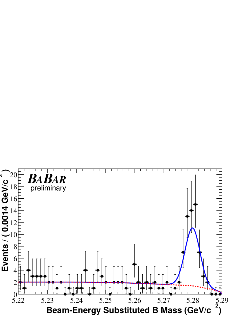
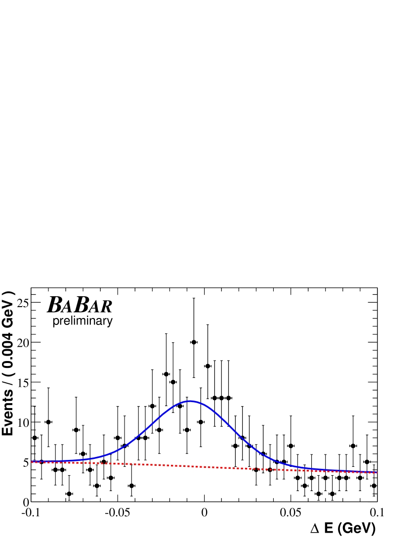
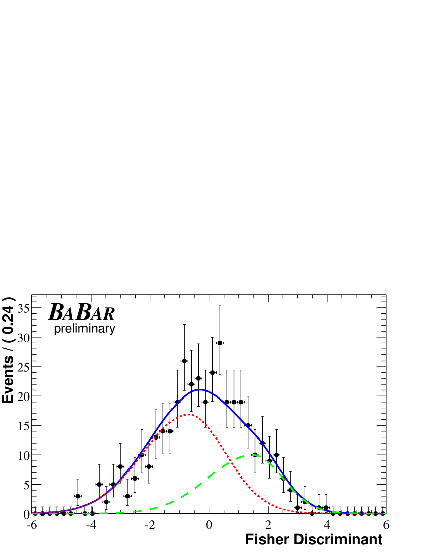
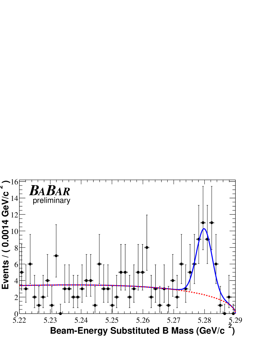
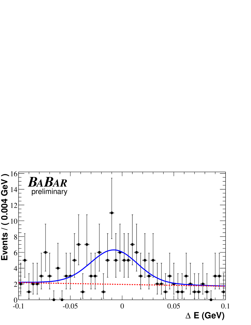
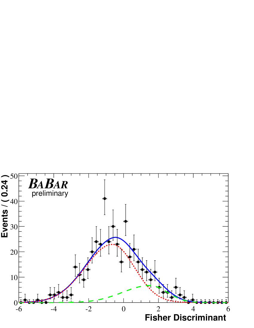
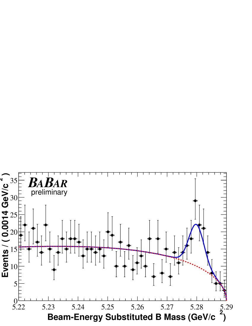
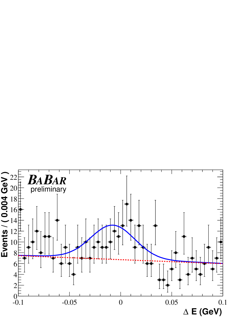
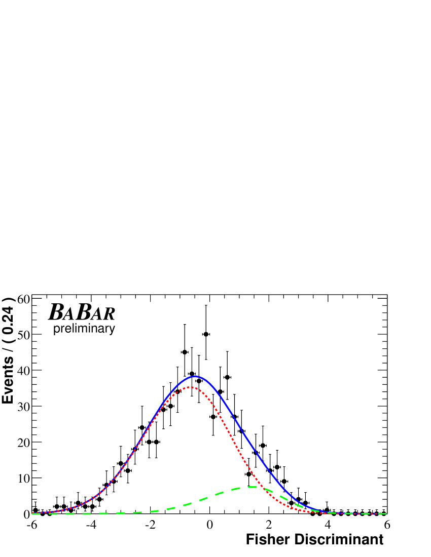
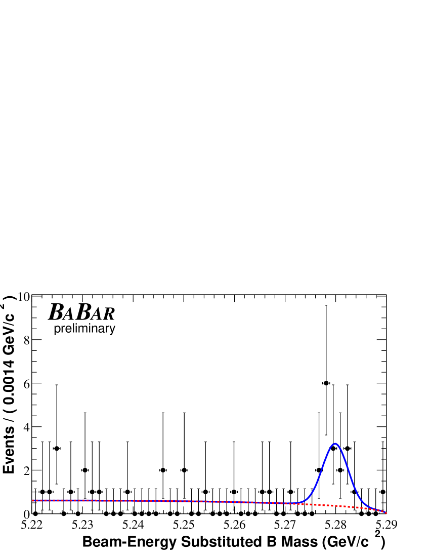
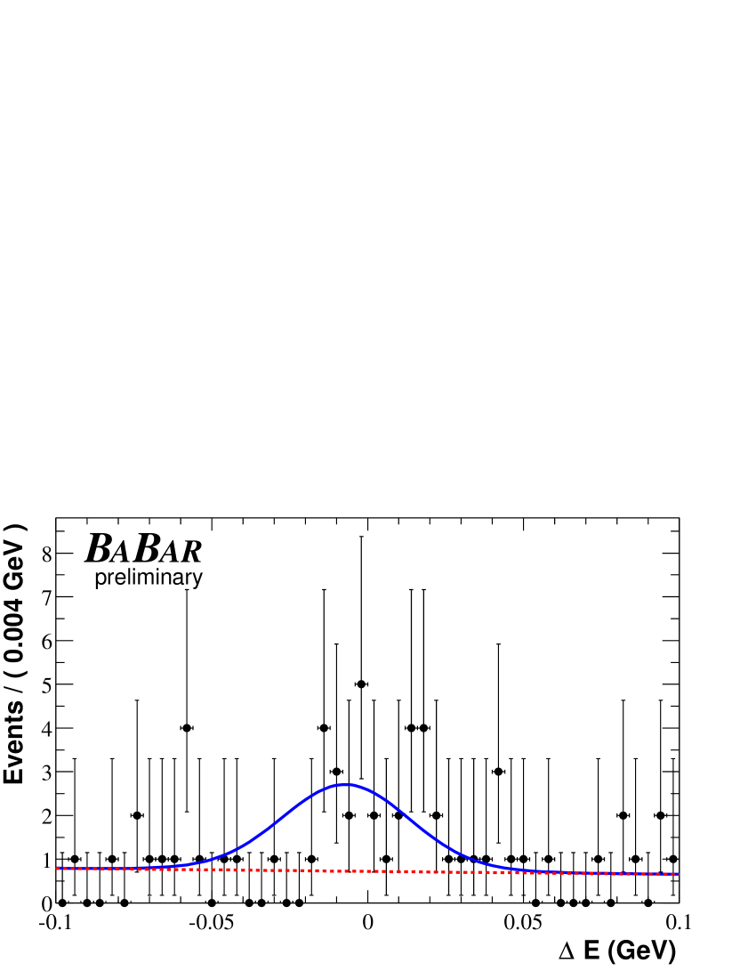
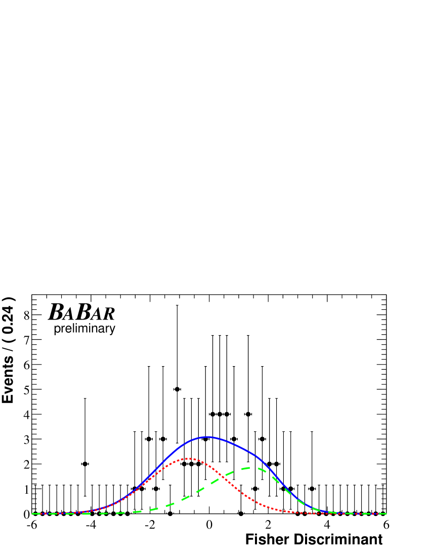
Figure 3: Projection plots in $m_{\rm ES}$, $\Delta E$ and ${\cal F}$, produced by selecting on the event likelihood ratio formed from the other two fit variables for (from top to bottom) regions V, VI, VII and VIII. The superimposed curve is a projection of the full fit with the background component shown as a dotted line and, for ${\cal F}$, the signal component shown as a dashed line.

The projection plots of $m_{\rm ES}$, $\Delta E$ and $\mathcal{F}$ for each region are shown in Figures 2 and 3. To produce these plots the projected variable is excluded from the likelihood functions and the ratio of the signal and background likelihoods for each event evaluated. The histograms are produced with a selection on this per–event likelihood ratio, where the selection value was chosen separately for each region to best illustrate the signal contribution. The projection of the fits onto that variable is then superimposed.

Figure 4 shows the Dalitz plot for data events within the signal region $5.2715<m_{ES}<5.2865{\mathrm{\,Ge\kern-1.00006ptV\!/}c^{2}}$ that have a per–event likelihood ratio, formed from the $\Delta E$ and $\mathcal{F}$ PDFs, greater than 5. To illustrate the expected background distribution, events passing the same likelihood selection but having a value of $m_{ES}$ between $5.25<m_{ES}<5.26{\mathrm{\,Ge\kern-1.00006ptV\!/}c^{2}}$ are shown alongside. The size of this sideband is chosen to contain approximately the same number of background events as are in the signal region. The mass intervals close to $J/\Psi$ and $\Psi(2S)$ are removed.

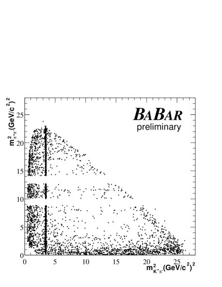
Figure 4: Dalitz plots showing the observed distribution in the signal $m_{\rm ES}$ region (left) and continuum background from the $m_{\rm ES}$ sideband (right) with the mass intervals close to $J/\Psi$ and $\Psi(2S)$ removed.

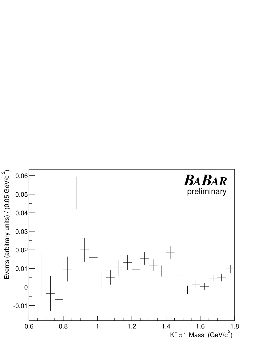
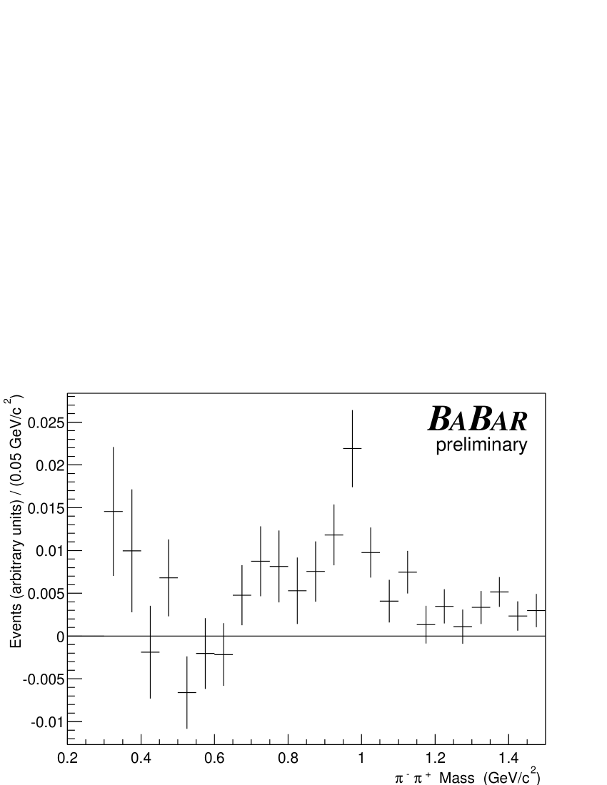
Figure 5: Background-subtracted and efficiency-corrected projections of the Dalitz plot in $m_{K\pi}$ and $m_{\pi\pi}$ in the ranges $0.6{\mathrm{\,Ge\kern-1.00006ptV\!/}c^{2}}<m_{K\pi}<1.8{\mathrm{\,Ge\kern-1.00006ptV\!/}c^{2}}$ and $0.2{\mathrm{\,Ge\kern-1.00006ptV\!/}c^{2}}<m_{\pi\pi}<1.5{\mathrm{\,Ge\kern-1.00006ptV\!/}c^{2}}$ with $J/\Psi$, $\Psi(2S)$ and $D^{0}$ vetoes applied. Peaks at the $K^{*0}(892)$ and $f_{0}(980)$ masses are clearly visible.

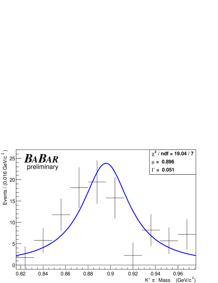
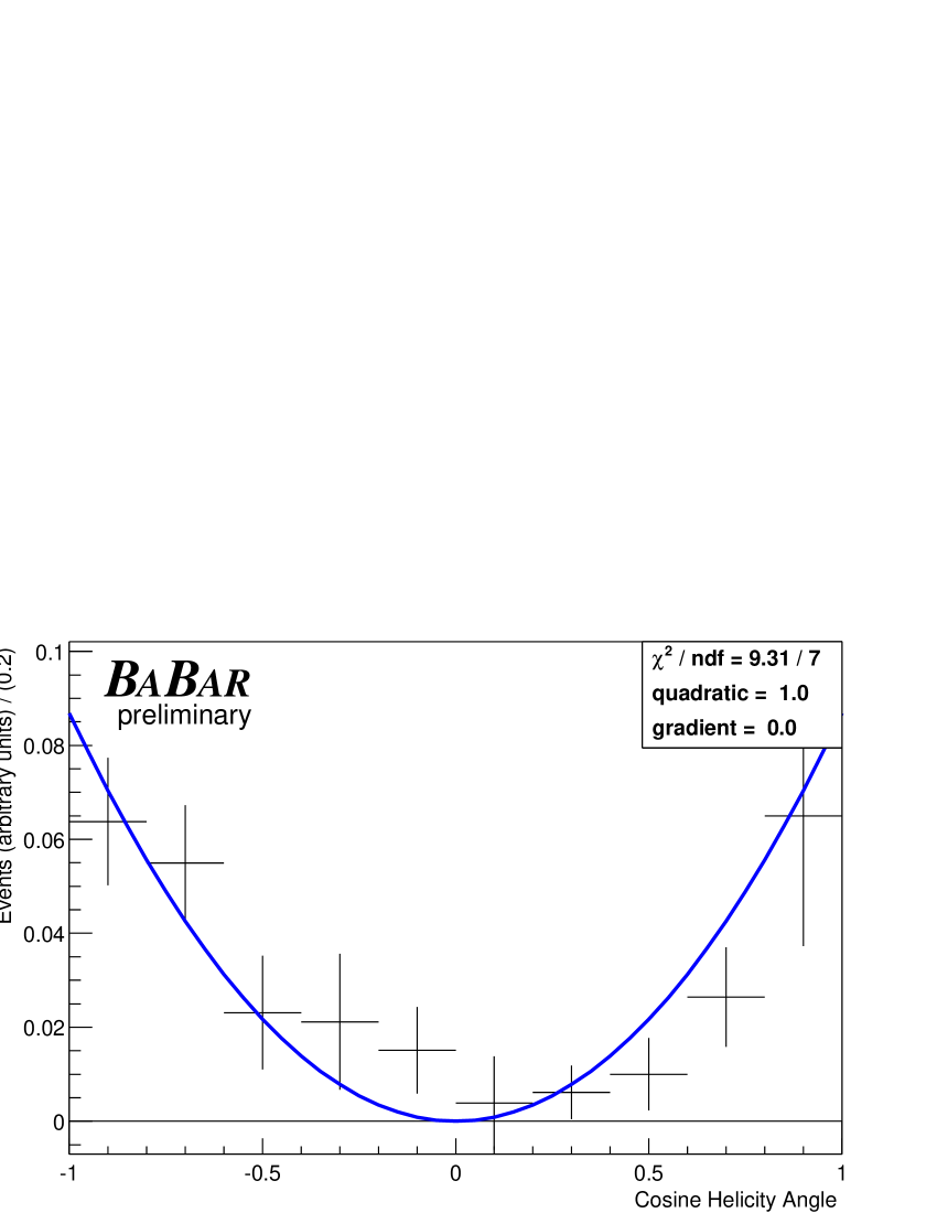
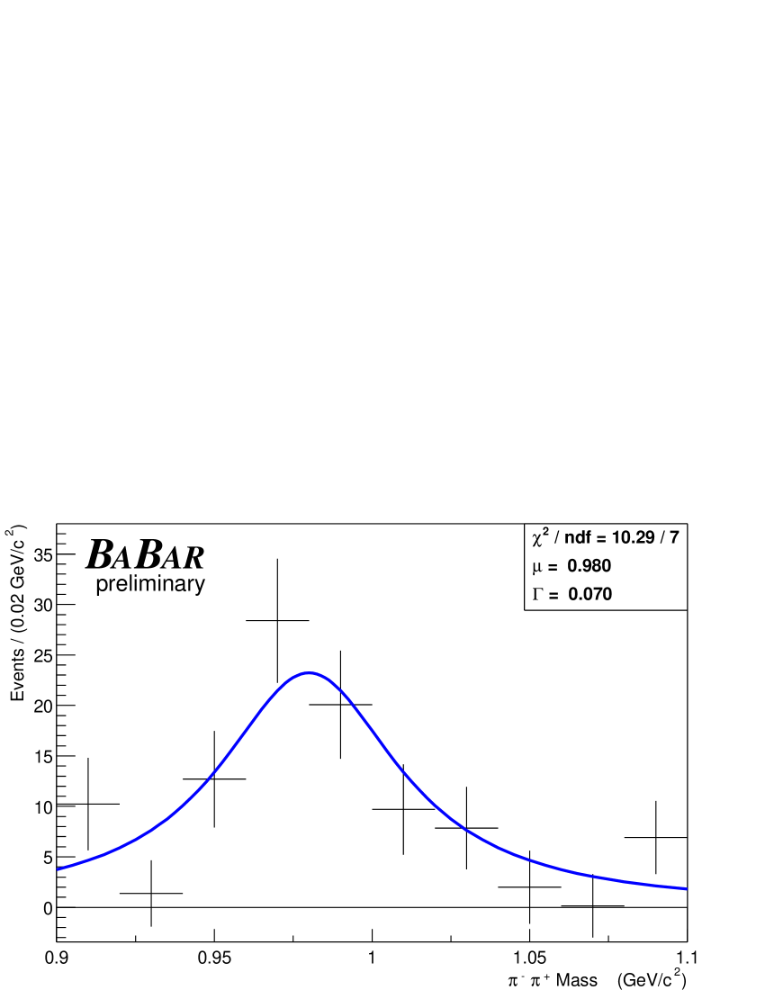
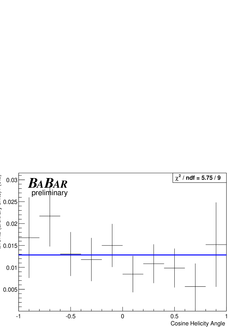
Figure 6: Projection plots of the resonant mass and cosine of the helicity angle for regions I and V. The background has been subtracted from all plots and, for the helicity distributions, a correction applied to each bin to account for the variation in reconstruction efficiency. The bold lines are the mass and helicity angle distributions that would be expected from the dominant resonant mode, $B^{+}\rightarrow\mbox{$K^{*0}(892)\pi^{+}$}$ for region I and $B^{+}\rightarrow\mbox{$\mbox{$f_{0}(980)$}K^{+}$}$ for region V with Breit-Wigner lineshapes and the masses and widths given in Table 3.

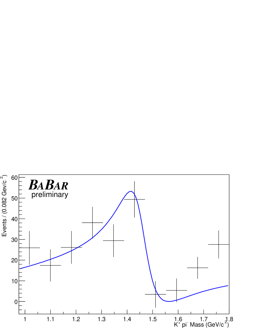
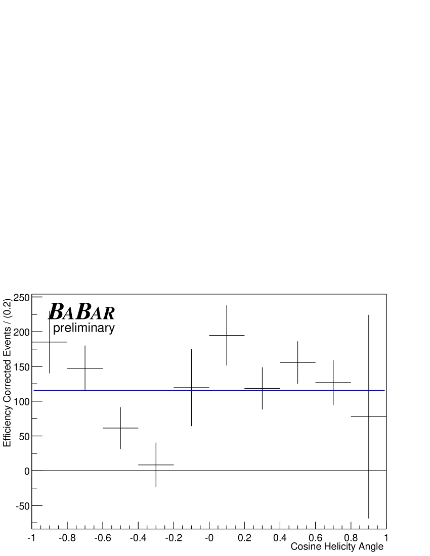
Figure 7: Projection plots of the resonant mass and cosine of the helicity angle for region II. The background has been subtracted from all plots and, for the helicity distributions, an efficiency correction applied to each bin. The mass parameterization obtained from the LASS experiment is superimposed as is a flat scalar distribution for the cosine of the helicity angle. The increase in event density above 1.6 ${\mathrm{\,Ge\kern-1.00006ptV\!/}c^{2}}$ is most likely caused by contributions from other higher-mass resonances.

Figure 5 shows background–subtracted projections of the Dalitz plot in $m_{K\pi}$ from $0.6{\mathrm{\,Ge\kern-1.00006ptV\!/}c^{2}}$ to $1.8{\mathrm{\,Ge\kern-1.00006ptV\!/}c^{2}}$ and $m_{\pi\pi}$ from $0.2{\mathrm{\,Ge\kern-1.00006ptV\!/}c^{2}}$ to $1.5{\mathrm{\,Ge\kern-1.00006ptV\!/}c^{2}}$. For these plots, signal events are obtained using a likelihood ratio selection on the $m_{ES}$ and ${\cal F}$ PDFs and the requirement $|\mbox{$\Delta E$}|<0.07\mathrm{\,Ge\kern-1.00006ptV}$, while the background is determined from the sideband $0.1<\mbox{$\Delta E$}<0.35\mathrm{\,Ge\kern-1.00006ptV}$. The $\kern 1.99997pt\overline{\kern-1.99997ptD}{}^{0}$, $J/\Psi$ and $\Psi(2S)$ vetoes are applied. The plots are efficiency–corrected using non–resonant $K^{+}\pi^{-}\pi^{+}$ Monte–Carlo data. Peaks at the $K^{*0}(892)$ and $f_{0}(980)$ masses are clearly visible. It is not clear what other channels are contributing, although there is a large signal in the region $1.1<m_{K\pi}<1.4{\mathrm{\,Ge\kern-1.00006ptV\!/}c^{2}}$. Figure 6 shows background–subtracted plots of the resonant mass and helicity angle distributions for regions I and V, where the $K^{*0}(892)$ and $f_{0}(980)$ resonances are expected to dominate. Only the helicity distributions have been efficiency–corrected as the efficiency does not vary over the range of the plotted mass distributions. The plots in Figure 6 have been overlaid with the distribution of the expected dominant resonance using Breit–Wigner line–shapes for the mass distributions, $\cos^{2}\theta_{H}$ for the $K^{*0}(892)$ angular distribution and a flat line for the scalar $f_{0}(980)$ angular distribution. There is good agreement between the overlaid and observed distributions indicating that the expected resonances are indeed dominant in these regions.

Figure 7 shows plots for region II produced in the same way. It is not clear from these distributions which resonances are present but it is unlikely that a single resonance can describe the $m_{K\pi}$ distribution. Superimposed is the effective–range parameterization used for the scalar $K^{*0}_{0}(1430)$ observed in the LASS experiment [12], using parameters taken from [13]. The agreement between this parameterisation and our observed distribution is good up to 1.6 ${\mathrm{\,Ge\kern-1.00006ptV\!/}c^{2}}$. The increase in event density above 1.6 ${\mathrm{\,Ge\kern-1.00006ptV\!/}c^{2}}$ is most likely caused by contributions from other higher resonances. The possibility that the $\kern 1.99997pt\overline{\kern-1.99997ptD}{}^{0}$ is contributing to this plot has been excluded by MC studies.

4.2 Branching Fractions

Regions III and VIII have negligible contributions from $B^{+}\rightarrow K^{+}\pi^{-}\pi^{+}$ channels other than $\kern 1.99997pt\overline{\kern-1.99997ptD}{}^{0}\pi^{+}$ and $\chi_{c0}K^{+}$, respectively. $\kern 1.99997pt\overline{\kern-1.99997ptD}{}^{0}\pi^{+}$ and $\chi_{c0}K^{+}$ do not contribute to other regions. The branching fractions for these channels are defined by:

$${\cal B}=\frac{\mbox{Y}}{\mbox{N${}_{B\kern 1.25995pt\overline{\kern-1.25995ptB}{}}$}\ \epsilon},$$ (2)

where Y is the signal yield and $\mbox{N${}_{B\kern 1.25995pt\overline{\kern-1.25995ptB}{}}$}=(61.6\pm 0.7)\times 10^{6}$ is the number of $B\kern 1.79993pt\overline{\kern-1.79993ptB}{}$ events in the sample. It is assumed the ${\mathchar 28935\relax\rm(4S)}$ decays equally to neutral and charged $B$ meson pairs. The reconstruction efficiency, $\epsilon$, is calculated using signal MC and is corrected for MC/data discrepancies in tracking and particle identification. We achieve efficiencies of $0.330\pm 0.017$ and $0.288\pm 0.017$ for $\kern 1.99997pt\overline{\kern-1.99997ptD}{}^{0}\pi^{+}$ and $\chi_{c0}K^{+}$, respectively, where the uncertainty is purely systematic.

For the other regions, we calculate the branching fractions from the measured yields taking into account the resonance cross–feed and model dependence. Y becomes a vector of the yields in each Dalitz region, $\cal{B}$ becomes a vector of the branching fractions and the efficiency becomes a matrix M the elements of which are the probability of an event of a particular decay to be found in a particular region.

$${\cal B}=\mbox{M}^{-1}\ \mbox{Y}/\mbox{N${}_{B\kern 1.25995pt\overline{\kern-1.25995ptB}{}}$}$$ (3)

Table 3: A summary of the model used to calculate branching fractions.

$i$	Decay Mode	Lineshape	Mass (${\mathrm{\,Me\kern-1.00006ptV\!/}c^{2}}$)	Width (${\mathrm{\,Me\kern-1.00006ptV\!/}c^{2}}$)	secondary BF (%)	Alternative Resonance
1	$K^{*0}(892)\pi^{+}$	BW	$896.10\pm 0.27$	$50.7\pm 0.6$	33.3	-
2	$K^{*0}_{0}(1430)\pi^{+}$	BW (LASS[12])	$1412\pm 6$	$294\pm 23$	$93\pm 10$	$K^{*0}_{2}(1430)$,$K^{*0}_{1}(1680)$
4	$\rho^{0}(770)K^{+}$	Blatt-W	$769.0\pm 0.9$	$150.9\pm 1.7$	100	-
5	$\mbox{$f_{0}(980)$}K^{+}$	BW (Flatté[18])	$980\pm 10$	$70\pm 30$	dominant	-
6	$f_{2}(1270)K^{+}$	BW	$1275\pm 12$	$185\pm 30$	$85\pm 2$	$f_{0}(1370)$, $f_{2}(1430)$
7	non-resonant	flat	all masses	-	-	-

The branching fractions measured depend on the model of resonances assumed in calculating the efficiency matrix M. We split M into two component matrices, P and $\epsilon$, such that each element $\mbox{M}_{ij}=\mbox{P}_{ij}\epsilon_{ij}$. The P matrix contains the event distribution around the Dalitz plot and the $\epsilon$ matrix contains the reconstruction efficiencies, so the model dependence is contained in the P matrix.

We assume one dominant contribution per region and the decay modes in the chosen resonance model are given in Table 3. The $K^{*0}(892)\pi^{+}$ and $\mbox{$f_{0}(980)$}K^{+}$ channels have been seen and there is evidence for $\rho^{0}(770)K^{+}$[14, 15]. For regions II, VI, VII, there are a number of possible contributions: for our model, we choose $K^{*0}_{0}(1430)$, $f_{2}(1270)$ and a flat non–resonant $K^{+}\pi^{-}\pi^{+}$. The masses and widths are taken from the Review of Particle Physics [16], and non–relativistic Breit–Wigner line–shapes are used for all channels except for the broad $\rho(770)$ resonance, where we use a relativistic Breit–Wigner lineshape with Blatt–Weisskopf damping [17]. The matrix element $\mbox{P}_{ij}$ gives the probability of an event of decay mode $i$ to be produced in region $j$ calculated using this model and including angular distributions and phase space. The elements are shown in Table 4. There are large uncertainties in this model: the dominant resonance is unknown in some regions, and there are uncertainties on the masses and widths of the resonances, as well as the choice of line–shapes. Alternative resonances, line–shapes and the uncertainties on resonance parameters are listed in Table 3. These cause uncertainties in P and therefore on the branching fractions. “Model” uncertainties on the branching fractions are evaluated that take into consideration all of these uncertainties in the model. There are also uncertainties in P due to the interference between the resonances and these “interference” uncertainties are also evaluated.

Table 4: The elements of the matrix P used to calculate the branching fraction central values, where $\mbox{P}_{ij}$ is the probability for an event of decay mode $i$ to be produced in region $j$.

	Region $j$
Decay Mode $i$	I	II	IV	V	VI	VII
1 $K^{*0}(892)\pi^{+}$	0.659	0.099	0.000	0.000	0.144	0.000
2 $K^{*0}(1430)\pi^{+}$	0.013	0.720	0.019	0.018	0.047	0.110
4 $\rho^{0}(770)K^{+}$	0.000	0.000	0.738	0.120	0.052	0.000
5 $\mbox{$f_{0}(980)$}K^{+}$	0.000	0.000	0.084	0.779	0.084	0.000
6 $f_{2}(1270)K^{+}$	0.008	0.031	0.020	0.064	0.741	0.111
7 high mass	0.013	0.127	0.032	0.029	0.074	0.642

The element $\epsilon_{ij}$ is defined as the number of decay–mode $i$ MC events with a candidate in region $j$ passing all the selection criteria divided by the number of decay mode $i$ events generated in region $j$. The $\epsilon$ matrix is calculated using resonant signal MC for $B^{+}\rightarrow\mbox{$K^{*0}(892)\pi^{+}$}$, $B^{+}\rightarrow\mbox{$\rho^{0}(770)K^{+}$}$ and $B^{+}\rightarrow\mbox{$\mbox{$f_{0}(980)$}K^{+}$}$, and non–resonant MC for other decay modes. These efficiencies have negligible dependence on the resonance line–shape; however, they are affected by the angular distribution. Corrections for MC/data discrepancies in particle identification and tracking are applied. The efficiencies are shown in Table 5.

Table 5: The elements of the efficiency matrix $\epsilon$, where $\epsilon_{ij}$ is the efficiency of decay mode $i$ events produced in region $j$ to pass the selection cuts. The statistical uncertainty on these numbers is negligible and the fractional systematic uncertainty is $5.8\%$ (see text for details).

	Region $j$
Decay Mode $i$	I	II	IV	V	VI	VII
1 $K^{*0}(892)\pi^{+}$	0.364	0.360	-	-	0.169	-
2 scalar $K^{*0}$	0.352	0.329	0.357	0.353	0.372	0.334
4 $\rho^{0}(770)K^{+}$	-	-	0.287	0.273	0.286	-
5 $\mbox{$f_{0}(980)$}K^{+}$	-	-	-	0.349	0.362	-
6 scalar $f$	0.352	0.329	0.357	0.353	0.372	0.334
7 high mass	0.352	0.329	0.357	0.353	0.372	0.334

Table 6: The branching fractions and uncertainties for the channels measured.

Channel	BF	uncertainties ($\times 10^{-6}$)
	($\times 10^{-6}$)	stat	sys	model	interference
$K^{*0}(892)\pi^{+},K^{*0}\rightarrow K^{+}\pi^{-}$	10.3	$\pm 1.2$	$\pm 0.7$	${}^{+0.4}_{-2.5}$	$\pm 0.6$
“higher $K^{*0}$”$\pi^{+},K^{*0}\rightarrow K^{+}\pi^{-}$	25.1	$\pm 2.0$	$\pm 2.9$	${}^{+9.4}_{-0.5}$	$\pm 4.9$
$\kern 1.99997pt\overline{\kern-1.99997ptD}{}^{0}$ $\pi^{+},\kern 1.99997pt\overline{\kern-1.99997ptD}{}^{0}\rightarrow K^{+}\pi^{-}$	184.6	$\pm 3.2$	$\pm 9.7$	-	-
$\rho^{0}(770)K^{+},\rho^{0}(770)\rightarrow\pi^{+}\pi^{-}$	3.9	$\pm 1.2$	${}^{+0.3}_{-0.6}$	${}^{+0.3}_{-3.2}$	$\pm 1.2$
$f_{0}(980)K^{+},f_{0}\rightarrow\pi^{+}\pi^{-}$	9.2	$\pm 1.2$	$\pm 0.6$	${}^{+1.2}_{-1.9}$	$\pm 1.6$
“higher $f$”$K^{+},f\rightarrow\pi^{+}\pi^{-}$	3.2	$\pm 1.2$	$\pm 0.5$	${}^{+5.8}_{-2.4}$	$\pm 1.5$
Non-resonant	5.2	$\pm 1.9$	${}^{+0.8}_{-1.8}$	${}^{+3.3}_{-7.5}$	$\pm 6.4$
$\chi_{c0}K^{+},\chi_{c0}\rightarrow\pi^{+}\pi^{-}$	1.5	$\pm 0.4$	$\pm 0.1$	-	-

Table 6 gives the branching fractions produced from the vector of yields with statistical, reconstruction–systematic, resonance–model and interference uncertainties.

4.2.1 Systematic Uncertainties

In most regions, the largest contribution to the reconstruction systematic uncertainty, between 3% and 11%, is from the uncertainties on the PDF parameters. The $B$ background subtraction uncertainty is below 6% for all channels except for $B^{+}\rightarrow\mbox{$\rho^{0}(770)K^{+}$}$ (18%) and non–resonant (32%), where it is dominant. The systematic uncertainties from track efficiency corrections (2.4%), particle identification efficiency (4.5%), $\cos\theta_{T}$ (2.8%) and the number of $B\kern 1.79993pt\overline{\kern-1.79993ptB}{}$ pairs (1.1%) are independent of the region considered. For “higher $f$” and “higher $K^{*0}$”, there is an additional contribution of 9% to account for the selection efficiency being measured using scalar MC though the true angular distribution of the contribution is unknown.

The model uncertainties include the effect of uncertainties in the resonance contributions, resonance masses, widths and line–shapes of the model, given in Table 3. The possibility that the dominant contribution to a region may be from another resonance is taken into account for $K^{*0}_{0}(1430)$ and $f_{2}(1270)$, where the alternative resonances are listed in Table 3. We consider the possibility that the component measured in Region VII does not extend into the other regions. We also allow for the possibility that the $f_{0}(980)$ resonance is described by the Flatté line–shape [18] and the $K^{*0}_{0}(1430)$ has the line–shape suggested by data from the LASS experiment [12][13] instead of the Breit–Wigner form. We estimate model uncertainties on the branching fractions by varying the model contributions, resonance parameters and line–shapes within the parameters given in Table 3, calculating a new $P$ matrix and recalculating the branching fractions. The model uncertainty is the quadratic sum of all the variations in the branching fraction due to these individual changes.

The effect of interference on the branching fractions is evaluated by generating many Dalitz plots with the observed branching fractions but with each contribution having a random phase and allowing interference, then measuring the branching fractions using the P matrix in the same way as done on the data. This produces a range of branching fractions for each channel with the correct branching fraction as the mean. The RMS variation is taken to be the uncertainty due to interference and this is shown in Table 6 under the column “interference”.

4.3 Conclusion

In conclusion, we have made preliminary measurements of the branching fractions for the following channels with a statistical significance greater than 5$\sigma$. This significance for a particular branching fraction ${\cal B}_{a}$ is evaluated by assuming that branching fraction is zero and minimizing, as a function of the other branching fractions, the $\chi^{2}$ separation of the measured yields and those obtainable from the branching fractions themselves. The significance is then given by $\sqrt{\chi^{2}({\cal B}_{a}=0)}$.

• $\mbox{${\cal B}$}(\mbox{$B^{+}\rightarrow\mbox{$K^{*0}(892)\pi^{+}$}$},K^{*0}\rightarrow K^{+}\pi^{-})=(10.3\pm 1.2^{+1.0}_{-2.7})\times 10^{-6}$,

• $\mbox{${\cal B}$}(\mbox{$B^{+}\rightarrow\mbox{$\mbox{$f_{0}(980)$}K^{+}$}$},f_{0}\rightarrow\pi^{+}\pi^{-})=(9.2\pm 1.2^{+2.1}_{-2.6})\times 10^{-6}$,

• $\mbox{${\cal B}$}(\mbox{$B^{+}\rightarrow\mbox{$\chi_{c0}K^{+}$}$},\chi_{c0}\rightarrow\pi^{+}\pi^{-})=(1.46\pm 0.35\pm 0.12)\times 10^{-6}$,

• $\mbox{${\cal B}$}(\mbox{$B^{+}\rightarrow\mbox{$\kern 1.99997pt\overline{\kern-1.99997ptD}{}^{0}\pi^{+}$}$},\kern 1.99997pt\overline{\kern-1.99997ptD}{}^{0}\rightarrow K^{+}\pi^{-})=(184.6\pm 3.2\pm 9.7)\times 10^{-6}$ and

• $\mbox{${\cal B}$}(B^{+}\rightarrow$“higher $K^{*0}$”$\pi^{+})=(25.1\pm 2.0^{+11.0}_{-5.7})\times 10^{-6}$, where “higher $K^{*0}$” means any combination of $K^{*0}_{0}(1430),K^{*0}_{2}(1430)$ and $K^{*0}_{1}(1680)$.

The first uncertainty is statistical and the second is systematic. This analysis has taken into account the uncertainty in the knowledge of the nature and parameterization of these resonances as well as interference between them, and these uncertainties are included (added in quadrature) in the above systematic value. Using the value of ${\cal B}(K^{*0}(892)\rightarrow K^{+}\pi^{-})=2/3$, we find $\mbox{${\cal B}$}(\mbox{$B^{+}\rightarrow\mbox{$K^{*0}(892)\pi^{+}$}$})=(15.5\pm 1.8^{+1.5}_{-3.2})\times 10^{-6}$, which is consistent with, and more precise than, previous measurements[14, 15]. The observation of the decay $B^{+}\rightarrow\mbox{$\mbox{$f_{0}(980)$}K^{+}$}$ is statistically significant, providing hints about the $f_{0}(980)$ production mechanism in the $B$ system. There is also a significant signal for $B^{+}\rightarrow$ “higher $K^{*0}$” $\pi^{+}$, which has a mass distribution which is partly described by the $K_{0}^{*0}(1430)$, as observed by the LASS experiment.

We give 90% confidence-level upper limits for the branching fractions of the following channels, including the non–resonant component. This upper limit is taken as the value of that branching fraction for which the minimum $\chi^{2}$ separation of the measured yields and those calculated from the branching fractions is 1.64.

• $\mbox{${\cal B}$}(\mbox{$B^{+}\rightarrow\mbox{$\rho^{0}(770)K^{+}$}$})<6.2\times 10^{-6}$,

• $\mbox{${\cal B}$}(B^{+}\rightarrow K^{+}\pi^{-}\pi^{+}$ non–resonant$)<17\times 10^{-6}$ and

• $\mbox{${\cal B}$}(B^{+}\rightarrow$“higher $f$”$K^{+})<12\times 10^{-6}$, where “higher $f$” means a combination of $f_{2}(1270)$, $f_{0}(1370)$ and $f_{2}(1430)$.

The tight limit on the non–resonant component means that it will be difficult to obtain the Unitarity Triangle angle $\gamma$ by the methods of Refs. [1] and [2].

5 Acknowledgements

We are grateful for the extraordinary contributions of our PEP-II colleagues in achieving the excellent luminosity and machine conditions that have made this work possible. The success of this project also relies critically on the expertise and dedication of the computing organizations that support BABAR. The collaborating institutions wish to thank SLAC for its support and the kind hospitality extended to them. This work is supported by the US Department of Energy and National Science Foundation, the Natural Sciences and Engineering Research Council (Canada), Institute of High Energy Physics (China), the Commissariat à l’Energie Atomique and Institut National de Physique Nucléaire et de Physique des Particules (France), the Bundesministerium für Bildung und Forschung and Deutsche Forschungsgemeinschaft (Germany), the Istituto Nazionale di Fisica Nucleare (Italy), the Foundation for Fundamental Research on Matter (The Netherlands), the Research Council of Norway, the Ministry of Science and Technology of the Russian Federation, and the Particle Physics and Astronomy Research Council (United Kingdom). Individuals have received support from the A. P. Sloan Foundation, the Research Corporation, and the Alexander von Humboldt Foundation.

References

- [1] N. G. Deshpande, G. Eilam, X. G. He and J. Trampetic, Phys. Rev. D 52 (1995) 5354.
- [2] S. Fajfer, R. J. Oakes and T.N. Pham, Phys. Lett. B 539 (2002) 67.
- [3] B. Aubert et al. [BABAR Collaboration], Nucl. Instr. Meth. A 479 (2002) 1.
- [4] R.H. Dalitz, Phil. Mag. 44 (1953) 1068.
- [5] R.A Fisher, Ann. Eugenics 7 (1936) 179; G. Cowan Statistical Data Analysis, (Oxford University Press, 1998) 51.
- [6] D. M. Asner et al. [CLEO Collaboration], Phys. Rev. D 53 (1996) 1039.
- [7] B. Aubert et al. [BABAR Collaboration], SLAC-PUB-9323 (2002).
- [8] B. Aubert et al. [BABAR Collaboration], SLAC-PUB-9232 (2002).
- [9] B. Aubert et al. [BABAR Collaboration], Phys. Rev. Lett. 87 (2001) 221802.
- [10] T. Skwarnicki, thesis, DESY F31-86-02 (1986).
- [11] H. Albrecht et al. [ARGUS Collaboration], Z. Phys. C 48 (1990) 543.
- [12] D. Aston et al., Nucl. Phys. B 296 (1988) 493.
- [13] A. Abele, Phys. Rev. D 57 (1998) 3860.
- [14] K. Abe et al. [Belle Collaboration], Phys.Rev. D 65 (2002) 092005.
- [15] B. Aubert et al. [BABAR Collaboration], SLAC-PUB-8981 (2001).
- [16] Particle Data Group, Phys. Rev. D 66 (2002) 010001.
- [17] J.M. Blatt and V.F. Weisskopf, Theoretical Nuclear Physics (Wiley, New York, 1952) 361.
- [18] S. M. Flatté, Phys. Lett. B 63 (1976) 224.