BUDKER-INP 2003-14
                                                                                         LC-DET-2003-054
BEAM ENERGY MEASUREMENT AT LINEAR COLLIDERS
USING SPIN PRECESSION 

Abstract

Linear collider designs foresee some bends of about 5-10 mrad. The spin precession angle of one TeV electrons on 10 mrad bend is $23.2$ rad and it changes proportional to the energy. Measurement of the spin direction using Compton scattering of laser light on electrons before and after the bend allows determining the beam energy with an accuracy about of $10^{-5}$. In this paper the principle of the method, the procedure of the measurement and possible errors are discussed. Some remarks about importance of plasma focusing effects in the method of beam energy measurement using Moller scattering are given.

1 INTRODUCTION

Linear colliders are machines for precision measurement of particle properties, therefore good knowledge of the beam energy is of great importance. At storage rings the energy is calibrated by the method of the resonant depolarization [1]. Using this method at LEP the mass of $Z$-boson has been measured with an accuracy of $2.3\times 10^{-5}$ [2]. Recently, at VEPP-4 in Novosibirsk, an accuracy of $\Psi$-meson mass of $4\times 10^{-6}$ has been achieved [3]. At linear colliders (LC) this method does not work and some other techniques should be used. The required knowledge of the beam energy for the t-quark mass measurement is of the order of $10^{-4}$, for the WW-boson pair threshold measurement it is $3\times 10^{-5}$ and ultimate energy resolution, down to $10^{-6}$, is needed for new improved Z-mass measurement. In other words, the accuracy should be as good as possible.

In the TESLA project [4] three methods for beam energy measurement are considered: magnetic spectrometer[5], Moller (Bhabha) scattering [6] and radiative return to Z-pole [7]. In the first method the accuracy $\Delta E/E\sim 10^{-4}$ is feasible, if a Beam Position Monitor (BMP) resolution of 100 nm is achieved. In the Moller scattering method an overall error on the energy measurement of a few $10^{-5}$ is expected [6, 4]. However, the resolution of this method may be much worse due to plasma focusing effects in the gas jet, see Sect. 8. In order to decrease these effects the gas target should be thin enough which results in a long measuring time.

In this paper a new method of the beam energy measurement is considered based on the precession of the electron spin in big-bend regions at linear colliders. It is not a completely new idea, after success of the resonant depolarization method people asked whether spin precession can be used for beam energy measurement at a linear collider. However, nobody has considered this option seriously [8] (see also remark in Sect.7).

2 Principle of the method

This method works if two conditions are fulfilled:

• electrons (and (or) positrons) at LC have a high a degree of polarization. If a second beam is unpolarized its energy can be found from the energy of the first beam using the acollinearity angle in elastic e⁺e^- scattering.

• there is a big (a few to ten mrads) bending angle between the linac and interaction point (IP). Such bend is natural in case of two interaction regions and in the scheme with the crab-crossing, otherwise the angle about 5 mrad can be intentionally added to a design.

During the bend the electron spin precesses around a vertical magnetic field. The spin angle in respect to the direction of motion $\theta_{s}$ varies proportionally to the bending angle $\theta_{b}$ [9]

$$\theta_{s}=\frac{\mu^{\prime}}{\mu_{0}}\gamma\theta_{b}\approx\frac{\alpha\gamma}{2\pi}\,\theta_{b},$$ (1)

where $\mu_{0}$ and $\mu^{\prime}$ are normal and anomalous electron magnetic momenta, $\gamma=E/m_{e}c^{2}$, $\alpha=e^{2}/\hbar c\approx 1/137$. For $E_{0}=1$ TeV and $\theta_{b}\sim 10$ mrad the spin rotation angle is 23.2 rad. The energy is found by measuring $\theta_{s}$ and $\theta_{b}$.

The bending angle $\theta_{b}$ is measured using geodesics methods and beam position monitors (BPM), $\theta_{s}$ can be measured using the Compton polarimeter which is sensitive to the longitudinal electron polarization, i.e. to the projection of the spin vector to the direction of motion. Assuming that the bending angle is measured very precisely (with relative accuracy smaller than the required energy resolution), the resulting accuracy of the energy is

$$\frac{\Delta E}{E_{0}}=\frac{\Delta\theta_{s}}{\theta_{s}}=\frac{2\pi\Delta\theta_{s}}{\alpha\gamma\theta_{b}}\sim\frac{0.43}{E_{0}(\mbox{TeV})\,\theta_{b}(\mbox{mrad})}\Delta\theta_{s}\,.$$ (2)

Possible accuracy of $\theta_{s}$ is discussed later.

A scheme of this method is shown in Fig.1.

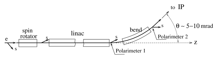
Figure 1: Scheme of the energy measurement at linear colliders using the spin precession.

The spin rotator at the entrance to the main linac can make any spin direction conserving the absolute value of the polarization vector $S$. A scheme of the rotator in the TESLA project is shown in Fig.2. It consists of three sections:

• an initial solenoid unit, which rotates the spin around the local longitudinal (z) axis by $\pm 90\,^{\circ}$;
  

• a horizontal arc which rotates the spin around the vertical axis by $90\,^{\circ}$ ($8^{\circ}$ bend for the 5 GeV beam energy after the damping ring);
  

• a final solenoid unit providing an additional rotation about z-axis by $\pm 90\,^{\circ}$.
  

The solenoid unit consists of two identical solenoids separated by short beamline whose (transverse) optics forms $(-I)$ transformation, thus effectively cancels the betatron coupling while the spin rotation of two solenoids add [4].

After the damping ring (DR) the electron spin $S$ has the vertical direction (perpendicular to the page plane). At the exit of the spin rotator it can have any direction.

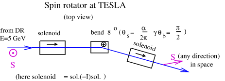
Figure 2: Scheme of the spin rotator, top view.

In the considered method the electron polarization vector should be oriented in the bending plane with high accuracy. Two Compton polarimeters measure the angle of the polarization vectors (before and after the bend). This allows one to find the beam energy.

A Compton polarimeter was used at SLC [10] and other experiments and will be used at the next LC for measurement of the longitudinal beam polarization [4]. The expected absolute accuracy of polarimeters is $\leq{\cal{O}}(1\%)$, but the relative variation of the polarization can be measured much more precisely.

3 Measurement of the spin angle

The longitudinal electron polarization is measured by Compton scattering of circularly polarized laser photons on electrons. After scattering off 1 eV laser photon the 500 GeV electron loses up to 90 % of its energy [11], namely these low energy electrons are detected for measurement of the polarization (see Fig.3)

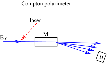
Figure 3: Compton polarimeter. M is the analyzing magnet, D the detector of electrons with large energy loss.

The energy spectrum of the scattered electrons in collisions of polarized electrons and photons is defined by the Compton cross section [12]

$${d\sigma\over dy}={d\sigma_{u}\over dy}[1+\mbox{${\cal{P}}_{\gamma}$}\mbox{${\cal{P}}_{e}$}\ F(y)],\;\;\;\;\;y=\frac{E_{0}-E_{e}}{E_{0}},$$ (3)

where $E_{e}$ is the scattered electron energy, the unpolarized Compton cross section

$${d\sigma_{u}\over dy}={2\sigma_{0}\over x}\left[{1\over 1-y}+1-y-4r(1-r)\right],$$

$$F(y)=\frac{rx(1-2r)(2-y)}{1/(1-y)+1-y-4r(1-r)},$$

$$x\approx\frac{4E_{0}\omega_{0}}{m^{2}c^{4}}=19\left[\frac{E_{0}}{\mbox{TeV}}\right]\left[\frac{\mbox{$\mu$m}}{\lambda}\right],\;\;r=\frac{y}{(1-y)x}\,,$$

$$\sigma_{0}=\pi r_{e}^{2}=\pi\left({e^{2}\over mc^{2}}\right)^{2}=2.5\times 10^{-25}\,\mbox{cm}^{2}\,,$$

$\mbox{${\cal{P}}_{e}$}\ =2\lambda_{e}$ is the longitudinal electron polarization (doubled mean electron helicity) and ${\cal{P}}_{\gamma}$ is the photon helicity, $\omega_{0}$ is the laser photon energy, $\lambda$ the wavelength. The minimum electron energy $E_{e,\,\min}=E_{0}/(x+1)$.

For example, at $E_{0}=250$ GeV and $\lambda=1\;\mu$m, $x\approx 4.8$, the minimum electron energy is about $0.18E_{0}$. The scattered photon spectra for this case are shown in Fig.4.

Figure 4: Spectrum of the Compton scattered electrons for various relative polarizations of laser end electron beams.

If one detect the scattered electrons in the energy range close to the minimum energies, the counting rate (or the analog signal in the polarimeter (see Sect.5.4) which is better suited for our task) is very sensitive to the product of laser and electron helicities, see Fig.4,

$$\dot{N}\propto(1-\mbox{${\cal{P}}_{\gamma}$}\mbox{${\cal{P}}_{e}$})+{\cal{O}}(0.2-0.3),$$ (4)

here ${\cal{O}}$ means “about”. In real experimental conditions some background is possible, according to estimates and previous experience at SLC [10] it can be made small compared to the signal.

The longitudinal electron polarization is given by $\mbox{${\cal{P}}_{e}$}\ =P_{e}\cos{\theta}$, where $P_{e}$ is the absolute value of the polarization, $\theta$ the angle between the electron spin and momentum. According to (4) the number of events in the polarimeter for a certain time is

$$N=A\cos{\theta}+B\,,$$ (5)

where $A\sim B$. This dependence is valid for all $\gamma$e processes [12], including Compton scattering with radiation corrections. Varying $\theta$ using the spin rotator one can find $N_{\max},N_{\min}$ corresponding to $\theta=0$ and $\pi$, then for other spin directions the angle can be found from the counting rate

$$\cos{\theta}=\frac{2N-(N_{\max}+N_{\min})}{N_{\max}-N_{\min}}\,.$$ (6)

Measurements of $\theta$ before ($\theta_{1}$) and after the bend ($\theta_{2}$) give the precession angle

$$\theta_{s}=\theta_{2}-\theta_{1}.$$ (7)

4 Statistical accuracy

The statistical accuracy can be evaluated from (6). Assuming that in both polarimeters $|\sin{\theta}|$ are chosen to be large enough (at any energy it is possible to make both $|\sin{\theta}|>0.7$) and $N_{\min},N_{\max}$ and $N$ are measured, the statistical accuracy of the precession angle is

$$\sigma(\theta_{s})<\frac{5}{\sqrt{N}},$$ (8)

where $N$ is the number of events in each polarimeter for the total time of measurement. If the Compton scattering probability is $10^{-7}$ and 30% of scattered electrons with minimum energies are detected, then the counting rate for TESLA is $2\cdot 10^{10}\times 14\,{\mbox{kHz}}\times 10^{-7}\times 0.3=10^{7}$ per second. The statistical accuracy of $\theta_{s}$ for 10 minutes run is $6\times 10^{-5}$. To decrease systematic errors one has to make some additional measurements (see the next section), which increase the measuring time roughly by factor of 3. Using (2) we can estimate the accuracy of the energy measurement for 1/2 hour run and $\theta_{b}=10$ mrad

$$\frac{\Delta E}{E_{0}}\sim\frac{2.5\times 10^{-6}}{E_{0}[\mbox{TeV}]}\,.$$ (9)

It is not necessary to measure the energy all the time. During the experiment one can make calibrations at several energies and then use measurements of the magnetic fields in bending magnets for calculation of energies at intermediate energy points. Between the calibrations it is necessary to check periodically the bending angle and stability of magnetic fields in the bending magnets.

If one spends only 1% of the time for the energy calibrations the overall statistical accuracy for $10^{7}$ sec running time will be much better than $10^{-5}$ for any LC energy and bending angles larger than several mrads.

In the experiment, it is important also to know the energy of each bunch in the train. Certainly, the dependence of the energy on the bunch number is smooth (after averaging over many trains) and can be fitted by some curve, therefore the energy of each bunch will be known only somewhat worse than the average energy.

It seems that the statistical accuracy is not a limiting factor, the accuracy will be determined by systematic errors.

5 Procedure of the energy measurement

Systematic errors depend essentially on the procedure of measurements. It should account for the following requirements:

• for the energy calibration polarized electrons and circularly polarized laser photons are used, but the result should not depend on the accuracy of the knowledge of their polarizations;

• the measurement procedure includes some spin manipulations using the spin rotator, the accuracy of such manipulation should not contribute to the result;

• change of the spin rotator parameters may lead to some variations of the electron beam sizes, position in the polarimeter and backgrounds, influence of these effects should be minimized.

Below we describe several procedures which can considerably reduce possible systematic errors.

5.1 Measurement of $N_{\max},N_{\min}$

The maximum and minimum signals in the polarimeter correspond to $\theta=0$ or $\theta=\pi$, see (5). To measure $N_{\max}$ one can use the knowledge of the accelerator properties and orient the spin in the forward direction with some accuracy $\delta\theta$. Our goal is to measure the signal with an accuracy at the level of $10^{-5}$. This needs $\cos{\,\delta\theta}<10^{-5}$ or $\delta\theta<5\times 10^{-3}$. It is difficult to guarantee such accuracy, it is better to avoid this problem. The experimental procedure which allows to reduce significantly this angle using minimum time is the following. In the first measurement instead of $\theta=0$ the spin has some small unknown angles $\theta_{x}$ and $\theta_{y}$ in horizontal and vertical planes, then the counting rate

$$N_{\max,1}\approx A+B\cos{(\sqrt{\theta_{x}^{2}+\theta_{y}^{2}})}\approx A+B(1-\theta_{x}^{2}/2-\theta_{y}^{2}/2)\,.$$ (10)

To exclude the uncertainty one can make some fixed known variations of $\theta_{x}$ and $\theta_{y}$ on about $10^{-2}$ rads based on knowledge of the spin rotator and accelerator parameters. The accuracy of such variations at the level of one percent is more than sufficient. Eq. (10) has 4 unknown variables: $A,\,B,\,\theta_{x},\,\theta_{y}$. To find them one needs 3 additional measurements. For example, in the second measurement one can make the variation $\Delta\theta_{x}$, in the third minus $\Delta\theta_{x}$ and in the fourth $\Delta\theta_{y}$. Solving the system of four linear equations one can find $\theta_{x}$, $\theta_{y}$, and after that make the final correction using the spin rotator which places the spin in the horizontal plane with very good accuracy (final angles are about 100 times smaller than the initial $\theta_{x}$, $\theta_{y}$, if the spin rotator makes the desired tilt with 1% accuracy) and collect larger statistics to determine $N_{\max}$. The minimum value of the signal, $N_{\min}$, is found in a similar way making variations around $\theta=\pi$.

5.2 Positioning the spin to the bending plane

For a precise measurement of the precession angle the spin should be kept in the bending plane. Initially, one can put the spin in this plane with an accuracy given by the knowledge of the system. The residual unknown angle $\theta_{y}$ can be excluded in a simple way. It is clear that the measured precession angle is a symmetrical function of $\theta_{y}$ and therefore depends on this small angle in a parabolic way. Let us take three measurements of the precession angle at $\theta_{y}$ (unknown) and $\theta_{y}\pm\Delta\theta_{y}$. These three measurement give three values of the precession angle $\theta_{s}(1)$, $\theta_{s}(2)$, $\theta_{s}(3)$ which correspond to three equidistant values of $\theta_{y}$. After fitting the results by a parabola one obtains the maximum (or may be the minimum, depending on the horizontal angles) value of $\theta_{s}$ which corresponds to the position of the spin vector in the bending plane. Using this result one can place the spin to the bending plane using the spin rotator with much higher accuracy and collect larger statistics for measurement of $\theta_{s}$.

Two additional remark to the later measurement:

1. The small vertical angle gives only the second order contribution to the precession angle $\theta_{s}$, therefore the absolute values of the variations $\Delta\theta_{y}$ in the second and third measurements should be known with rather moderate accuracy. Furthermore, $\pm\Delta\theta_{y}$ give the scale and the final variation is taken as a certain part of $\Delta\theta_{y}$ (which is easier than some absolute value). For example, if $\Delta\theta_{y}\sim 3\times 10^{-2}$ and on the final step we add a part of this angle with an accuracy 3 %, the final $\theta_{y}$ will be less than $10^{-3}$ ($<5\times 10^{-3}$ is needed, Sect.5.1).

2. Varying $\theta_{y}$ one can make an uncontrolled variation of $\theta_{x}$ at the entrance to the bending system. However, it makes no problem since we measure the difference of the $\theta_{x}$ measured before and after the bend.

5.3 Variation of electron beam sizes and position in polarimeters

Geometrical parameters of the electron beam can depends somewhat on spin rotator parameters. In existing designs of the spin rotators [4] these variations are compensated, but some residual effects can remain. These dependences should be minimized by proper adjustment of the accelerator; additionally they can be reduced by taking laser beam sizes much larger than those of the electron beams.

The laser-electron luminosity (proportional to Compton scattering probability) is given by

$$L=\frac{N_{e}N_{L}\nu}{4\pi\sqrt{(\sigma_{y,L}^{2}+\sigma_{y,e}^{2})[(\sigma_{z,L}^{2}+\sigma_{z,e}^{2})(\theta/2)^{2}+(\sigma_{x,L}^{2}+\sigma_{x,e}^{2})]}},$$ (11)

where $\theta$ is the collision angle, $\sigma_{i,e}$ are the electron beam sizes, $\sigma_{i,L}$ are the laser beam sizes, $N_{e},\,N_{L}$ are the number of particles in the electron and laser beams and $\nu$ is the beam collisions rate. This formula is valid when the Rayleigh length $Z_{R}$ (the $\beta$-function of the laser beam) is larger than the laser bunch length. Assuming that electron beam sizes are much smaller than those of the laser, the laser beam is round ($\sigma_{x,L}=\sigma_{y,L}$) and its sizes are stable we get

$$L=\frac{N_{e}N_{\gamma}\nu}{4\pi\sigma_{y,L}\sqrt{(\sigma_{z,L}^{2}(\theta/2)^{2}+\sigma_{y,L}^{2})}}\times$$

$$\left(1-\frac{\sigma_{y,e}^{2}}{2\sigma_{y,L}^{2}}-\frac{\sigma_{z,e}^{2}\theta^{2}+4\sigma_{x,e}^{2}}{2(\sigma_{z,L}^{2}\theta^{2}+4\sigma_{y,L}^{2})}\right)$$ (12)

Electron beam sizes at maximum LC energies (but not at the interaction point) are of the order of $\sigma_{z,e}=100-300$ $\mu$m, $\sigma_{x,e}\sim 10\,\mbox{$\mu$m}$,  $\sigma_{y,e}\sim 1\,\mbox{$\mu$m}$. In order to reduce the dependence on the electron beam parameters laser beam sizes should be much larger than those of the electron beams, i.e. $\sigma_{y,L}\gg\sigma_{y,e}$ and $\sigma_{z,L}\theta\gg\sigma_{x,e}$. Under these conditions the collisions probability depends on variations of the transverse electron beam sizes as follows

$$\frac{\Delta L}{L}=\left(\frac{\sigma_{y,e}}{\sigma_{y,L}}\right)^{2}\frac{\Delta\sigma_{y,e}}{\sigma_{y,e}}+\left(\frac{2\sigma_{x,e}}{\sigma_{z,L}\,\theta}\right)^{2}\frac{\Delta\sigma_{x,e}}{\sigma_{x,e}}$$ (13)

Our goal is to measure the signal in the polarimeters with an accuracy about $10^{-4}$. Let the transverse electron beam size varies on 10 %. In order to decrease the corresponding variations of $L$ down to the desired level one should take

$$\sigma_{y,L}=\sigma_{x,L}\approx 30\,\sigma_{y,e}\sim 30\;\mbox{$\mu$m},$$ (14)

$$\sigma_{z,L}\theta\approx 30\times 2\sigma_{x,e}\sim 600\,\mbox{$\mu$m}.$$ (15)

Deriving (11) we assumed $\sigma_{z,L}<Z_{R}$, the latter can be found from (14) using the relation $\sigma_{y,L}\equiv\sqrt{\lambda Z_{R}/4\pi}$. It gives

$$\sigma_{z,L}<Z_{R}=4\pi\sigma^{2}_{y,L}/\lambda\sim 1\;\mbox{cm},$$ (16)

where $\lambda=1$ $\mu$m was assumed.

Eqs.(15) and (16) do not fix the collision angle. As the laser beam is cylindrical, the collision probability will be the same if one takes long bunch and small angle or short bunch and large angle. For example, in the considered case of $\sigma_{x,e}=10\;\mbox{$\mu$m}$ and $\sigma_{y,e}=1\;\mbox{$\mu$m}$, one can take $\sigma_{z,L}\sim 0.5Z_{R}\sim 0.5$ cm (longest as possible according to (16)) and $\theta\sim 0.1$.

The required laser flash energy ($A$) can be found from (11) and relations

$$L\sigma_{c}=kN_{e}f\;\;\;\;\;A=\omega_{0}N_{\gamma}\,,$$

where $k$ is the probability of Compton scattering (for electrons) and $\sigma_{c}$ is the Compton cross section. Leaving the dominant laser terms which were assumed to be 30 times larger than the electron beam sizes, we find the required laser flash energy

$$A\approx\omega_{0}\frac{4\pi\sigma_{x,e}\sigma_{y,e}(30)^{2}k}{\sigma_{c}}.$$ (17)

For example, for $\lambda=1\;\mbox{$\mu$m}$ ($\omega_{0}=1.24$ eV), $\sigma_{x,e}=10$ $\mu$m, $\sigma_{y,e}=1$ $\mu$m, $k=10^{-7}$ and $\sigma_{c}=1.7\times 10^{-25}\;\mbox{cm}^{2}$ (for $E_{0}=250\;\mbox{GeV})$ we get $A=1.3\times 10^{-4}$ J. The average laser power at 20 kHz collision rate is 2.5 W (no problem).

Another way to overcome this problem is a direct measurement of this effect and its further correction. In this case the laser beam can be focused more tightly. In order to do this one should take the photon helicity be equal to zero and change the electron spin orientation in the bending plane using the spin rotator. As the Compton cross section depends on the product of laser and electron circular polarization the signal in the polarimeters may be changed only due to the electron beam size effect. To make sure that circular polarization of the laser in the collisions point is zero with a very high accuracy one can take the electron beam with longitudinal polarization close to maximum and vary the helicity of laser photons using a Pockels cell. The helicity is zero when counting rate in the polarimeter is $0.5(N_{\max}+N_{\min})$. These data can be used for correction of the residual beam-size effect.

The position of the electron beam in the polarimeters can be measured using beam position monitors (BPM) with a high accuracy. The trajectory can be kept stable for any spin rotator parameters using the BPM signals and corrector magnets.

5.4 Detector

As a detector of the Compton scattered electrons one can use the gas Cherenkov detector successfully performed in the Compton polarimeter at SLC [10]. It detects only particles traveling in the forward direction and is blind for wide angle background. The expected number of particles in the detector from one electron bunch is about 1000. Cherenkov light is detected by several photomultipliers.

To correct nonlinearities in the detector one can use several calibration light sources which can work in any combination covering the whole dynamic range.

For accurate subtraction of variable backgrounds (constant background is not a problem) one can use events without laser flashes. Main source of background is bremsstrahlung on the gas. Its rate is smaller than from Compton scattering and does not present a problem.

5.5 Measurement of the bending angle

We assumed that the bending angle can be measured with negligibly small accuracy. Indeed, beam position monitors can measure the electron beam position with submicron accuracy. In this way one can measure the direction of motion. Measurements of the angle between two lines separated by several hundreds meters in air is not a simple problem, but there is no fundamental physics limitation at this level. For example, gyroscopes (with correction to Earth rotation) provide the needed accuracy.

6 Systematic errors

Some possible sources of systematic errors were discussed in the previous section. Realistic estimation can be done only after the experiment. Measurement of $\Delta\theta_{s}$ (averaged over many pulses) on the level $10^{-4}$ does not look unrealistic. The statistical accuracy can be several times better and allows to see some possible systematic errors.

If systematics are on the level $10^{-4}$, the accuracy of the energy calibration according to (2) is about

$$\frac{\sigma_{E}}{E_{0}}\sim\frac{0.5\times 10^{-4}}{\theta_{b}[\mbox{mrad}]E_{0}[\mbox{TeV}]}.$$ (18)

7 Measurement of the magnetic field vs spin precession.

There is a good question to be asked: maybe it is easier to measure magnetic field in all bending magnets instead of measurement of the spin precession angle [8]?

Yes, it is more a straightforward way. However, we discuss the method which potentially allows an accuracy of the LC energy measurement of about $10^{-5}$. Bending magnets in the big-bends should be weak enough, $B\sim 10^{3}$ G, to preserve small energy spread and emittances. Who can guarantee $10^{-2}$ G accuracy of the magnetic field when the Earth field is about 1 G?

8 Some remarks on the beam energy measurement using Moller (Bhabha) scattering

In this method electrons are scattered on electrons of a gas target, the energy is measured using angles and energies of both final electrons in a small angle detector [6, 4]. For LEP-2 energy the estimated precision was about 2 MeV.

Here I would like to pay attention to one effect in this method which was not discussed yet. It is a plasma focusing of electrons. The electron beam ionizes the gas target, free electron quickly leave the beam volume while ions begin to focus electrons. Deflection of electrons in the ion field can destroy the beam quality and affect the energy resolution.

Let us make some estimations of this effect for $E_{0}=90$ GeV which was considered in the original proposal for LEP-2 [6], but for linear collider beams. The angle of the scattered electron for the symmetric scattering is $\theta=\sqrt{2m_{e}c^{2}/E}\sim 3$ mrad. The Moller (Bhabha) cross section for the forward detector considered in  [6] is 15 (4) $\mu$b. The dominant contribution to the energy spread of measured energy is due to the Fermi motion of the target electron [6]: $\sigma_{E}/E=3.6\cdot 10^{-3}$. Somewhat smaller contribution gives the intrinsic beam energy spread. Let us take the combined energy resolution (for one event) to be equal to $\sigma_{E}/E=5\cdot 10^{-3}$. In order to obtain 0.5 MeV statistical accuracy in $10^{3}$ sec the luminosity of beam interactions with the $H_{2}$ target should be about $L=0.6\,(2.4)\cdot 10^{32}$ cm^-2s^-1 for $e^{-}$ ($e^{+}$), or approximately $10^{32}$ (in [6] $L=4\cdot 10^{31}$ was assumed).

The luminosity is $L=N_{e}\nu nl$, where $N_{e}\sim 10^{10}$ is the number of particles in the electron bunch, $\nu\sim 10^{4}$ the collision rate, $n$ the density of electrons in the target and $l$ is the target thickness. This gives the required depth of the gas target $n\,l\sim 10^{18}$ cm^-2.

Let us consider now ionization of the hydrogen target by the electron beam. The relativistic particle produces in $H_{2}$ at normal pressure about 8.3 ions/cm, this corresponds to the cross section (per one electron) $\sigma_{i}=8.3/(2\times 2.68\cdot 10^{19})=1.5\cdot 10^{-19}\;$cm². The total number of ions produced by the beam $N_{i}=N_{e}\sigma_{i}nl=10^{10}\times 1.5\cdot 10^{-19}\times 10^{18}=1.5\cdot 10^{9}$, that is 15% of the number of particles in the beam.

For the vertical (smallest) transverse beam size smaller than the plasma wavelength and the density of the beam higher than the plasma density, all plasma electrons are pushed out from the beam. These conditions correspond to our case. The maximum deflection angle of the beam electrons in the ion field is

$$\Delta\theta\sim\frac{2r_{e}N_{i}}{\sigma_{x}\gamma}.$$ (19)

The horizontal beam size $\sigma_{x}=\sqrt{\epsilon_{n,x}\beta/\gamma}\sim\sqrt{3\cdot 10^{-4}\times 3000/2\cdot 10^{5}}\sim 2\times 10^{-3}$ cm. Here we assumed that $\beta\sim 300\,\sqrt{E_{0}\mbox{(GeV)}}$ cm. The resulting deflection angle is $\Delta\theta\sim 2\cdot 10^{-6}$.

The energy resolution (systematic error) due to the plasma focusing is $\sigma_{E}/E\sim 2\Delta\theta/\theta\sim 1.4\times 10^{-3}$, that two order of magnitude larger than our goal (about $10^{-5}$).

The angular spread in the beam in the vertical direction is $\sqrt{\epsilon_{n,y}/(\beta_{y}\gamma)}\sim\sqrt{3\cdot 10^{-6}/(3000\times 2\cdot 10^{5})}\sim 0.7\cdot 10^{-7}$ rad that is 30 times smaller than the deflection angle, so the beam after the gas jet can not be used for the experiment.

To avoid these problems one can take the gas target thinner by two orders of magnitude. Then in the considered example the statistical accuracy $10^{-5}$ for electrons is achieved in 4.5 hours. Note that at such beam thickness one can measure the energy and run experiment simultaneously.

The cross sections of the Moller and Bhabha scattering depends on the energy as $1/E^{2}$ which leads to increase of the measuring time for higher energy. However one can increase the target thickness and allow some degradation of the resolution. The optimum is reached when the statistical error is equal to the systematic one. The systematic error is $\Delta E/E\propto\Delta\theta/\theta\propto nl/(\sigma_{x}\gamma)/(1/\sqrt{\gamma})\propto nl/\gamma^{1/4}.$ The statistical error is $\sigma_{E}/E\propto 1/\sqrt{N}\propto 1/\sqrt{n\sigma l\,t}\propto\gamma/\sqrt{nlt}$. At optimum conditions $\sigma_{E}/E\propto\gamma^{7/12}/t^{1/3}$. So, for the same scanning time, a ten times increase of energy leads to 3.8 times increase of the energy resolution.

Several additional remarks on plasma effects which were not discussed here but may be important:

• For positrons plasma effects are smaller because the ionization is confined in the beam channel and the scattered electrons after a short travel in the gas target get $\Delta y>\sigma_{y}$ where the ion and electron fields cancel each other;

• in the above consideration the secondary ionization in the beam field was ignored;

• it is well known that short beams in plasma create strong longitudinal wakefields, about $E_{z}\sim\sqrt{n_{p}\,\mbox{[cm${}^{-3}$]}}$ eV/cm, which decelerates the beam. This effect may be not negligible in the considered problem.

9 Discussion and Conclusion

The method of beam energy measurement at linear colliders using spin precession has been considered. The accuracy on the level of a few $10^{-5}$ looks possible.

In this paper we considered only the measurement of the average beam energy before the beam collision. Experiments will require not this energy but the distribution of collisions on the invariant mass. The beam energy spread at linear colliders is typically about $10^{-3}$, but much larger energy spread and the shift of the energy gives beamstrahlung during the beam collision. An additional spread in the invariant mass distribution gives also an initial state radiation. So, the luminosity spectrum will consist of the narrow peak with the width determined by the initial beam energy spread and the tail due to beamstrahlung and initial state radiation. This spectrum in relative units can be measured from the acollinearity of Bhabha events [13, 14, 15]. The absolute energy scale is found from the measurement of average beam energy before the beam collisions which was discussed in the present paper. Namely the narrow peak in the luminosity spectrum provides such correspondence. The statistical accuracy of the acollinearity angle technique is high, some questions remain about systematic effects.

References

- [1] S.I. Serednyakov, A.N. Skrinsky, G.M. Tumaikin, Yu.M. Shatunov, Zh.Eksp.Teor.Fiz.71 (1976) 2025; Ya.S. Derbenev, A.M. Kondratenko, S.I. Serednyakov, A.N. Skrinsky, G.M. Tumaikin, Yu.M. Shatunov, Part. Accel. 10 (1980) 177.
- [2] Particle Data Group, Phys. Rev. D, 66 (2002).
- [3] V.M. Aulchenko et al. (KEDR collaboration), hep-ex/030605, to be published in Phys. Lett..
- [4] TESLA Technical Design Report. Part 4. A Detector for TESLA, Ed. R. Heuer et al., DESY-2001-011, ECFA-2001-209, Mar 2001.
- [5] J. Kent, IEEE Particle Accel. Conference, Chicago, IL,1989, edited by F.Bennet and J.Kopta (IEEE, Piscatway, NJ, 1989).
- [6] C. Cecchi, J.H. Field, T. Kawamoto, Nucl. Instrum. Meth. A385 (1997) 445.
- [7] OPAL collaboration, G. Abbiendi et al., OPAL physics notes No. PN476 and No. OPAL-PN493, CERN, 2001.
- [8] E. Torrence, Talk at Snowmass 2001 (eConf C010630:E3010,2001).
- [9] B. Berestersky, E. Lifshitz, L. Pitaevsky, Quantum Electrodynamics (Pergamont press, New York, 1982).
- [10] R. King, SLAC-Report-452, 1994, A. Lath, SLAC-Report-454, 1994.
- [11] I.F. Ginzburg, G.L. Kotkin, V.G. Serbo, and V.I. Telnov, Nucl. Instr. &Meth., 205 (1983) 47.
- [12] I.F. Ginzburg, G.L. Kotkin, S.L. Panfil, V.G. Serbo, and V.I. Telnov. Nucl. Inst. Meth., A219 (1984) 5.
- [13] M.N. Frary and D.J. Miller, DESY-92-123A, 1992, p.379.
- [14] K. Monig. LC-PHSM-2000-060, contribution to 2nd ECFA/DESY Study 1998-2001, 1353-1361, edeted by T.Behnke et al..
- [15] S.T. Boogert, D.J. Miller, Proc. Intern. Workshop on Physics and Detectors at Linear Colliders (LCWS2002), Jeju Island, Korea, 2002, edited by J.S. Kang and S.K. Oh, p.509, hep-ex/0211021.