Measurements of Rare B Decays at BABAR 

Abstract

We present the results of searches for rare B meson decays. The measurements use all or part of a data sample of about 88 million $\Upsilon(4S)\rightarrow B{\bar{B}}$ decays collected between 1999 and 2002 with the BABAR detector at the PEP-II asymmetric energy B Factory at the Stanford Linear Accelerator Center. We study a variety of decays dominated by electromagnetic, electroweak and gluonic penguin transitions, and report measurements of branching fractions and other quantities of interest.

1 Introduction

Measurements[1, 2, 3, 4, 5, 6, 7, 8, 9, 10, 11, 12, 13, 14, 15, 16] of rare B meson branching fractions have been performed using the BABAR[17] detector. B decays in which CKM favored amplitudes are suppressed or forbidden are sensitive to penguin amplitudes and hence to possible non-Standard Model effects arising from new particles participating in internal loops. In addition to probes for new physics, many of these modes are also crucial to the full constraint of the “Unitarity Triangle”. As the definition implies, rare decays typically have branching fractions of less than $10^{-4}$. The present data sample of roughly 88 million $B{\bar{B}}$ pairs allows for measurements or stringent limits on many such modes.

1.1 Flavor and the Quark Sector of the Standard Model

The complex CKM[18] matrix describes the coupling of the charged weak transition $q\rightarrow W^{*+}q^{\prime}$, which is proportional to $V^{*}_{qq^{\prime}}$. The non-diagonality of this matrix expresses the fact that the Weak isospin doublet members $(b^{\prime},s^{\prime},d^{\prime})$ are states of mixed flavor. We can thus view the CKM matrix as the transformation between the mass and flavor eigenstates of the quarks

$$\left(\begin{array}[]{c}d^{\prime}\\ s^{\prime}\\ b^{\prime}\end{array}\right)=\left(\begin{array}[]{ccc}V_{ud}&V_{us}&V_{ub}\\ V_{cd}&V_{cs}&V_{cb}\\ V_{td}&V_{ts}&V_{tb}\end{array}\right)\left(\begin{array}[]{c}d\\ s\\ b\end{array}\right).$$ (1)

The unitarity condition implies that there are four free parameters in this matrix, one of which is a phase. It is through this phase that the Standard Model can accommodate CP violation. In particular, the orthogonality requirement between the first and third columns requires

$$V_{ud}V_{ub}^{*}+V_{cd}V_{cb}^{*}+V_{td}V_{tb}^{*}=0,$$ (2)

which can be expressed geometrically as the so called “Unitarity Triangle” shown in Figure 1. Information about each side and angle is accessible through a variety of measurements in the B meson system. The angles are measured through time-dependent decay rate asymmetries, and the sides via direct or indirect measurements of the CKM matrix elements. Measurement of all the components of the Unitarity Triangle over-constrains the triangle, and thus provides a test of the Standard Model (SM).

Fig. 1: The Unitarity Triangle determined from the orthogonality of the first and third columns of the CKM matrix. Also shown are B meson processes which yield information about each side and angle.

2 The BABAR Detector

A detailed description of the BABAR detector can be found elsewhere[17]. Charged particle momenta are measured in a tracking system that consists of a 5-layer double-sided silicon micro-strip vertex tracker (SVT) and a 40-layer drift chamber (DCH) filled with an (80:20) mixture of helium and isobutane. The tracking volume is contained within the 1.5T magnetic field of a superconducting solenoid. The combined track momentum resolution is $\sigma_{p_{T}}/p_{T}=0.13\%\times p_{T}+0.45\%$. The primary charged hadron identifiation device is a detector of internally reflected Cerenkov radiation (DIRC). The typical separation of kaons and pions due to their measured Cerenkov angle $\theta_{C}$ varies from 8$\sigma$ at 2 GeV/c to 2.5$\sigma$ at 4 GeV/c, where $\sigma$ is the average $\theta_{C}$ resolution. Specific ionization energy loss (dE/dx) measurements in the DCH and SVT also contribute to charged hadron identification for particle momenta less than 0.7 GeV/c. Photons are detected in an electromagnetic calorimeter (EMC) consisting of 6580 Thallium doped CsI crystals arranged in barrel and forward end-cap sub-detectors. The $\pi^{0}$ mass resolution in on average about 7 MeV/c². Muons and long-lived neutral hadrons are detected within the instrumentation of the solenoid flux return (IFR) which consists of alternating layers of iron and resistive plate chambers.

3 Common Analysis Features

3.1 Data sample

The analyses described here use all or part of a data sample consisting of approximately 88 million pairs of $\Upsilon(4S)\rightarrow B{\bar{B}}$ decays, corresponding to a detector exposure of about 81 fb^-1. An additional sample of 9.6 fb^-1 taken about 40 MeV below the peak of the $\Upsilon(4S)$ resonance (“off-resonance”) is used by many analyses to study $e^{+}e^{-}\rightarrow q{\bar{q}}$ “continuum” backgrounds.

3.2 B Meson Reconstruction

B mesons produced from $\Upsilon(4S)$ decays are identified via their unique kinematics. Because the mass of the $B$ meson pair is nearly that of the $\Upsilon(4S)$, they are produced nearly at rest ($p^{*}_{B}\approx 325$ MeV/c). Use of the beam energy in constraining the kinematics serves to reduce the resolution of theses variables.

The conservation of energy can be expressed as:

$$\Delta E=E^{*}_{B}-E^{*}_{beam},$$ (3)

where $E^{*}_{beam}$ is the single beam energy in the center-of-mass (CM) frame. $E^{*}_{B}$ is the measured energy of the $B$ candidate in the CM. Correctly reconstructed $B$ candidates have $\Delta E$ distributed around zero with a resolution ranging from 15 to 80 MeV. The energy resolution of the $B$ decay products dominates the resolution of this variable. Continuum background in this variable is well described by a monotonically decreasing low order polynomial. Figure 2 shows the $\Delta E$ distribution for a typical rare mode after all selection criteria have been applied (except that on $\Delta E$).

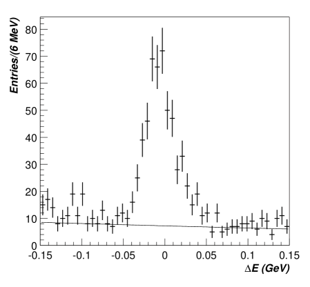
Fig. 2: $\Delta E$ distribution for charged $B$ decays to three charged kaons. All candidate selection criteria have been applied except that on $\Delta E$. The solid line shows the expected continuum background level.

We express momentum conservation as:

$$m_{ES}=\sqrt{E^{*2}_{beam}-{\vec{p}}^{*2}_{B}}.$$ (4)

Here $m_{ES}$ is the “beam-energy substituted mass”, with ${\vec{p}}^{*}_{B}$ the $B$-candidate momentum in the CM. Correctly reconstructed $B$ candidates have $m_{ES}$ equal to the $B$ meson mass, with a resolution of about 2.5-3.0 MeV/c², which is dominated by the beam energy spread. The continuum background shape in $m_{ES}$ is parameterized by a threshold function[19] with a fixed endpoint given by the average beam energy. Figure 3 shows the $M_{ES}$ distribution for a typical rare mode after all other selections have been applied.

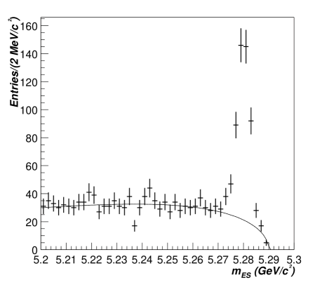
Fig. 3: $m_{ES}$ distribution for charged $B$ decays to three charged kaons. All candidate selection criteria have been applied except that on $m_{ES}$. The solid line shows the expected continuum background level.

In addition to the kinematics of the $B$ meson, signal events are selected by making requirements on the decay products. $B$ daughter resonances are required to have invariant masses within a restricted range typically determined by resolution and the need to leave sufficient sideband to determine background levels. Particle identification requirements are made to select some particles and veto sources of background.

3.3 Background Suppression

All rare analyses suffer from substantial backgrounds, and a variety of techniques are employed to reduce this to manageable levels. In general, backgrounds from other $B$ decays are small. Decays resulting from CKM favored $b\rightarrow c$ transitions have heavier daughters and higher multiplicity final states than do CKM suppressed decays. In order to wrongly reconstruct such a decay as a rare signal, one must typically lose a particle from the true $B$ decay, resulting is a substantial shift in the candidate’s $\Delta E$. The only exception to this is for rare modes with high final state multiplicities, in which indications of some background have been observed. While $B$ decays from other CKM suppressed transitions have similar kinematics and multiplicities to that of a rare signal, such modes are rare themselves, and require only limited suppression in most analyses. Where $B$ backgrounds are present, they typically populate the sidebands of the $\Delta E$ distribution, but have tails that reach into the signal region as illustrated in Figure 4

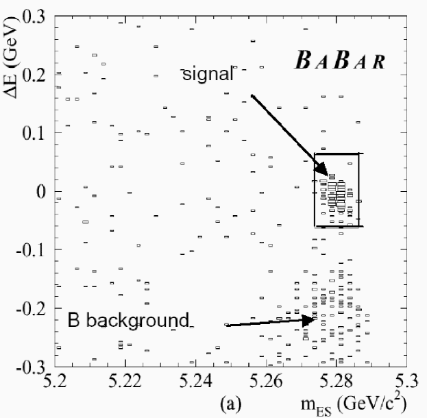
Fig. 4: Typical $m_{ES}$ vs $\Delta E$ distribution after event selection. The signal populates the region around $m_{ES}=5.280$ and $\Delta E=0$. Continuum background populates the entire plane. $B$ background populates the $\Delta E$ sideband.

For all the modes discussed here, the primary background is due to random particle combinations arising from continuum quark-antiquark production. Although the probability for any given continuum event to satisfy a signal selection is quite small, the numbers favor the continuum. The total production cross section for light quarks (including charm) under the $\Upsilon(4S)$ is about 3.5 nb, but only 1 nb for the $\Upsilon(4S)$ itself. For a mode with an expected branching fraction of order 10^-6 this means that continuum events are produced at a rate well in excess of 10⁶ times that of the signal.

In order to control continuum backgrounds, one typically exploits the fact that while the $B$ meson pairs are produced near threshold in $\Upsilon(4S)$ decays, the light and charm quark pairs which comprise the continuum are produced with a great deal of excess energy. The result is that for true $B$ meson decays, the decay products entering the detector are distributed isotropically in the CM, while the continuum background exhibits a “jet-like” topology, with a strong correlation between the $B$ candidate decay and jet axes.

The first topological variable typically employed is the angle $\theta_{T}$ between the thrust axes of the $B$ candidate and the remaining particles in the event. The sphericity axes may be used almost interchangeably. The distribution of $|cos\theta_{T}|$ is nearly uniform for true $B$ mesons, but is strongly peaked near 1 for continuum background as is illustrated in Figure 5. If additional background rejection is required, one may consider the remaining event shape information, such as the angles between the $B$ thrust and decay axes and the beam as well as the angular energy flow in the event, and combine it into an optimized quantity using a neutral network or a Fisher discriminant. An example of the the separation power of a Fisher discriminant after a thrust cut has been made can be found in Figure 6.

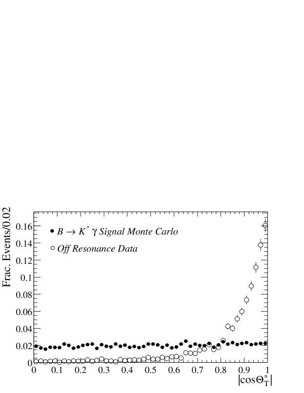
Fig. 5: Signal and background distributions of $|cos\theta_{Thrust}|$ for a typical $B$ meson decay. The signal distribution (solid histogram) is uniform, reflection the random orientation between the $B$ candidate thrust axis and the thrust axis of the rest of the event. The background (open points) is strongly peaked at one due to the strong correlation between these two axes in fake $B$ candidates arising from random particle combinations in the continuum.

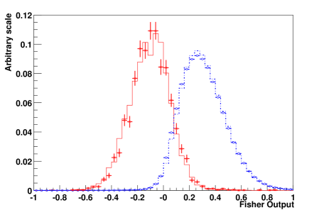
Fig. 6: Distribution of Fisher discriminant for data control mode (solid points), control mode signal Monte Carlo (solid histogram), continuum data (open points) and continuum Monte Carlo (dashed histogram) after a cut on $|cos\theta_{Thrust}|$. The Fisher and Thrust angle are strongly correlated, thus the separation will depend strongly on the thrust cut made.

3.4 Signal Extraction

All rare analyses at BABAR are performed “blind”, meaning that signal yields are hidden from the analyzer until the analysis has been peer reviewed and determined to be in a final form. These steps are taken to avoid experimenter’s bias.

There are two primary methods in which signal event yields are extracted; the event counting analysis, and the maximum likelihood fit. Detection efficiencies determined from signal Monte Carlo simulations and data control samples are used to convert yields into branching fraction measurements. Equal production of charged and neutral $B$’s from the $\Upsilon(4S)$ decay are assumed throughout.

In the event counting analysis, a set of selection criteria are defined to select a signal region of the parameter space. The criteria are optimized with respect to expected signal and background yields to produce a measurement of the greatest possible statistical significance. Systematic uncertainties may figure into this process, but they are usually negligible for rare modes. The selection are applied to the data, and the population of signal region is counted. An estimated background is subtracted to determine the signal event yield. The background yield is typically determined by measuring the density of events in a sideband region and projecting that density into the signal region.

In the maximum likelihood fit method signal yields are determined by an unbinned extended maximum likelihood fit to a set of observables. These typically include $m_{ES}$, $\Delta E$, event shape variables and, where appropriate, $B$ daughter resonance invariant masses and particle identification information. The probability ${\cal P}_{i}({\vec{x}}_{j};{\vec{\alpha}}_{i})$ for a given hypothesis $i$ is the product of probability density functions (PDFs) for each of the variables ${\vec{x}}_{j}=(m_{ES},\Delta E,{\rm Fisher},...)$ given the set of parameters ${\vec{\alpha}}_{i}$. The hypotheses $i$ are signal, continuum background and sometimes $B$ background for each final state in the fit. The likelihood function is given by a product over all events $N$ and the signal and background components:

$${\cal L}=\frac{e^{-\sum_{i}n_{i}}}{N!}\prod_{j=1}^{N}{\cal L}_{j},\;\;\;{\cal L}_{j}=\sum_{i}n_{i}{\cal P}_{i}({\vec{x}}_{j};{\vec{\alpha}}_{i}).$$ (5)

The $n_{i}$ are the numbers of events for each hypothesis. The values of the yields (and any free parameters in the PDFs) are taken as those which maximize the likelihood function. Unit change in $-2ln{\cal L}$ defines the one standard deviation statistical uncertainties on the free parameters in the fit. The statistical significance of the signal yield is determined from the change in $-2ln{\cal L}$ when the signal yield is forced to zero. If no statistically significant signal is found (more than 4 standard deviations), a 90% confidence level upper limit may be obtained by requiring:

$$\frac{\int_{0}^{n_{UL}}{\cal L}(n)dn}{\int_{0}^{\infty}{\cal L}(n)dn}=0.9.$$ (6)

Full and toy Monte Carlo simulations are used to verify that the fit is unbiased.

The accuracy with which the PDFs describe the data is of utmost importance in the likelihood fit. Background PDFs are determined by fits to off-resonance and sideband data. Signal PDFs are determined primarily from signal Monte Carlo simulations, but ultimately rely on data control samples to verify their validity.

4 Electromagnetic Penguins

Electromagnetic penguins consist of the class of amplitudes in which an external photon is emitted by one of the virtual particles participating in the loop through which the $b\rightarrow s(d)$ transition proceeds. This is illustrated in Figure 7. Such diagrams are relatively clean from a theoretical perspective, and a variety of information can be gather from measurements of decays dominated by these amplitudes. The decay $B\rightarrow K^{*}\gamma$ was the first penguin to be observed[20]. Measurements of its branching fraction provides a test of QCD, and direct CP violation in this mode would be an indication of new physics. The decay rate ratio of $B\rightarrow\rho\gamma$ to $B\rightarrow K^{*}\gamma$ is sensitive to the ratio of $|\frac{V_{td}}{V_{ts}}|$. The photon energy spectrum from measurements of $b\rightarrow s\gamma$ provides information on the mass and Fermi motion of the $b$ quark within the $B$ meson.

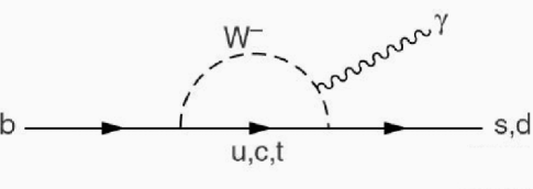
Fig. 7: Feynman diagram for an electromagnetic penguin amplitude.

In the analysis of these modes, in each case there is a requirement of a high energy isolated photon. The calorimeter cluster is required to have a profile consistent with an electromagnetic shower, and the candidate photon must not be consistent with having originated from a $\pi^{0}$ or $\eta$ decay. Further details and results of each analysis are presented below.

4.1 Measurement of $B\rightarrow K^{*}\gamma$

The analysis of $B\rightarrow K^{*}\gamma$[1] has been performed on a data sample corresponding to approximately 22 million $B{\bar{B}}$ pairs recorded in 1999-2000. The $K^{*}\gamma$ final state is reconstructed in all four $K^{*}$ decay modes. Stringent identification requirements are placed on charged kaons. Invariant mass requirements are placed on both $K^{*}$ and $K^{0}_{S}$ candidates. The $K^{0}_{S}$ is also required to have a decay vertex displaced from the $e^{+}e^{-}$ interaction point. Since the $B$ meson is a pseudoscalar, angular momentum conservation requires that the $K^{*}$ is polarized. The absolute value of the cosine of the $K^{*}$ helicity angle is required to be less than 0.75. Continuum background is suppressed with cuts on the absolute values of the cosines of the thrust and $B$ flight angles, both of 0.80.

After cutting on $\Delta E$, the signal yield is determined from an unbinned maximum likelihood fit to the $m_{ES}$ distribution, shown for each $K^{*}$ decay mode in Figure 8. Branching fraction and direct CP asymmetry results are shown in Table 1[21].

	${\cal B}(B^{0}\rightarrow K^{*0}\gamma)$	${\cal B}(B^{+}\rightarrow K^{*+}\gamma)$	$A_{CP}$
Theory[22, 23, 24]	$7.5\pm 3.0$	$7.5\pm 3.0$	$|A_{CP}|<0.005$
BABAR	$4.23\pm 0.40\pm 0.22$	$3.83\pm 0.62\pm 0.22$	$-0.17<A_{CP}<0.08$
			@90% CL

Table 1: Results of the branching fraction and direct asymmetry analysis of $B\rightarrow K^{*}\gamma$. In each result, the first uncertainty is statistical, the second systematic. Branching fractions are in units of $10^{-5}$.

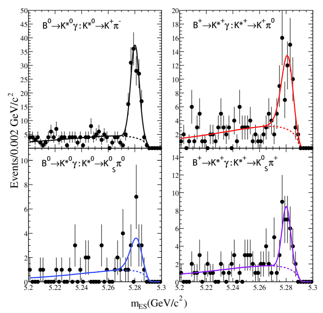
Fig. 8: The $m_{ES}$ distribution for $B\rightarrow K^{*}\gamma$ in each of the $K^{*}$ decay modes. All selection criteria have been applied. The solid curve is the combined signal and background PDF shape, the dashed is the background only.

4.2 Search for $B\rightarrow\rho\gamma$ and $B\rightarrow\omega\gamma$

The analysis of the $\rho\gamma$ and $\omega\gamma$ final states[2] is significantly more challenging than that of $K^{*}\gamma$. The predicted branching fractions are about 50 times smaller than for $K^{*}\gamma$. Both the $\rho$ and the $\omega$ have significantly more background under their peaks than does the $K^{*}$, and the rho is much broader. In addition to continuum background, these modes also potentially suffer cross-feed background from $K^{*}\gamma$, other $b\rightarrow s\gamma$ processes and from $B\rightarrow\rho\pi^{0}$.

A neutral network containing information from event shape, $\Delta t$ and flavor tagging is used to control continuum background. $K^{*}\gamma$ feed-across is vetoed using particle identification. After these selection criteria are applied, the signal yield for each final state is extracted using a unbinned maximum likelihood fit to $m_{ES}$, $\Delta E$, and the $\rho/\omega$ invariant mass. Studies of generic $B{\bar{B}}$ Monte Carlo show that the expected $B$ background is quite small, so the fit includes components only for signal and continuum background. Background from $B$ decays is considered as a systematic uncertainty.

The results of this analysis applied to a sample of 84 million $B{\bar{B}}$ pairs can be found in table 2. If isospin symmetry is assumed, all three modes can be combined to produce an upper limit of ${\cal B}(B\rightarrow\rho\gamma)<1.9\times 10^{-6}$ @ 90% CL. This result can be used to place on upper limit on CKM parameters $|\frac{V_{td}}{V_{ts}}|<0.036$ @ 90% CL. A discussion of theoretical errors can be found in Ali and Parkhomonko[24].

	${\cal B}(B^{0}\rightarrow\rho^{0}\gamma)$	${\cal B}(B^{+}\rightarrow\rho^{+}\gamma)$	${\cal B}(B^{0}\rightarrow\omega\gamma)$
Theory[24]	$0.5-0.75$	$0.8-1.5$	$0.5-0.75$
BABAR	$<1.4$	$<2.3$	$<1.2$

Table 2: Results of the branching fraction analysis of $B\rightarrow\rho\gamma$ and $\omega\gamma$. Branching ratios are in units of $10^{-6}$. Upper limits are at 90% CL.

4.3 Semi-Inclusive Measurement of $b\rightarrow s\gamma$

This analysis[3] of 22 million $B{\bar{B}}$ pairs is a study of a collection of exclusive final states with a kaon plus up to four pions, no more than one of which may be neutral. Because $b\rightarrow s\gamma$ is a two-body decay process, the photon energy $E_{\gamma}$ in the $B$ rest frame is related to the recoil hadronic mass, $M_{Had}$:

$$E_{\gamma}=\frac{M_{B}^{2}-M_{Had}^{2}}{2M_{B}}.$$ (7)

Fits to the measured spectra of both of these quantities can be used to determine the total branching ratio for $B\rightarrow X_{s}\gamma$[25]. In addition to constraining new physics contributions to the underlying amplitude, parameters associated with heavy quark effective theory (HQET) are also extracted in the analysis. These parameters are critical to reducing theory errors in the extraction of $V_{ub}$ and $V_{cb}$.

Measured branching fractions as a function of $M_{Had}$ and $E_{\gamma}$ can be found in Figure 9. Analysis of these spectra yield results:

$${\bar{\Lambda}} = 0.37\pm 0.09(stat)\pm 0.07(syst)\pm 0.10(model)\;{\rm GeV/c^{2}}$$

$$m_{b} = 4.79\pm 0.08(stat)\pm 0.10(syst)\pm 0.10(model)\;{\rm GeV/c^{2}}$$

$$\lambda_{1} = -0.24^{+0.03}_{-0.04}\;(stat)\pm 0.02(syst)\;^{+0.15}_{-0.21}(model)\;{\rm GeV/c^{2}}$$

$${\cal B}(b\rightarrow s\gamma) = 4.3\pm 0.5(stat)\pm 0.8(syst)\pm 1.3(model)\times 10^{-4}.$$ (8)

Fig. 9: Hadronic recoil mass and photon energy spectra for the semi-inclusive analysis of $b\rightarrow s\gamma$. Errors are statistical only.

4.4 Fully-Inclusive Measurement of $b\rightarrow s\gamma$

Much of the uncertainty in the semi-inclusive $b\rightarrow s\gamma$ analysis arises from theoretical errors. HQET implies a duality between the quark and hadron level of an interaction, which implies that parton level rate for $b\rightarrow s\gamma$ is the same as the inclusive rate for $B\rightarrow X_{s}\gamma$. These two issues motivate the fully inclusive analysis technique.

This analysis[4] is performed on a sample of 60 million $B{\bar{B}}$ pairs. Photons in the range $1.5<E^{*}_{\gamma}<3.5$ GeV are analyzed. These photons are required to meet the selection criteria described above. To suppress continuum background the event is required to have a lepton flavor tag which strongly selects true $B{\bar{B}}$ decays. Such a selection induces no model dependency into the analysis as it only applies to the “other” $B$ in the decay. In addition to particle identification criteria, fake leptons are further rejected by requiring large missing energy in the event, which is normally associated with semi-leptonic $b\rightarrow c$ transitions. To obtain additional discrimination, the angular separation between the lepton and the photon is required not to be small. Event topology in the form of the Fox-Wolfram moments in also employed to reduce background from the continuum. Backgrounds are estimated using off-resonance data and $B{\bar{B}}$ Monte Carlo.

The $E_{\gamma}$ spectra for on-resonance data and the predicted background are shown in Figure 10.

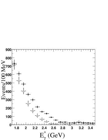
Fig. 10: The $E^{*}_{\gamma}$ distribution of on-resonance data (solid points) and background expectations for the fully inclusive analysis of $B\rightarrow X_{s}\gamma$. Errors are statistical only.

The photon energy range $2.1<E^{*}_{\gamma}<2.7$ GeV is considered to reduce model dependencies. The branching fraction for $B\rightarrow X_{s}\gamma$ is measured in this region and then extrapolated to the full spectrum:

$${\cal B}(B\rightarrow X_{s}\gamma)=3.88\pm 0.36(stat)\pm 0.37(syst)^{+0.43}_{-0.23}(model)\times 10^{-4}.$$ (9)

5 Electroweak Penguins

As the name suggests, Electroweak penguins are amplitudes that proceed via loops involving photons, $W$ or $Z$ bosons. Such processes are strongly suppressed in the Standard Model, and as such, are excellent windows onto potential new physics. Well controlled theoretical uncertainties aid in this sensitivity. We discuss the analysis of four such final states here: $K^{(*)}\ell^{+}\ell^{-}$[5], $\ell^{+}\ell^{-}$[6], $K\nu{\bar{\nu}}$[7], and $\gamma\gamma$[8].

5.1 Measurement of $B\rightarrow K^{(*)}\ell^{+}\ell^{-}$

The flavor-changing neutral current decays $B\rightarrow K\ell^{+}\ell^{-}$ and $B\rightarrow K^{*}\ell^{+}\ell^{-}$ have predicted branching fractions on the order $10^{-6}-10^{-7}$[26]. The leading diagrams for this decay are electroweak penguin and box diagrams, and can be found in Figure 11.

Fig. 11: Leading Electroweak penguin and box diagrams for the decay $B\rightarrow K^{(*)}\ell^{+}\ell^{-}$.

The decay rate for $B\rightarrow K^{(*)}\ell^{+}\ell^{-}$ is rather sensitive to the presence of new physics. In particular, certain extensions to the SM can vary the rate by more than a factor of two. In addition to the decay rate, kinematic distributions accessible with higher statistics, such as the boson $q^{2}$ distribution ($m_{\ell\ell}^{2}$) and the forward-backward asymmetry in the $K^{*}$ channel are of considerable interest as they are also quite sensitive to non-SM physics, and are less model dependent than the overall rate.

The experimental challenge in this analysis is to control the various sources of background. Background from $B\rightarrow$ charmonium decays which have the same final state particles are control by vetoing regions in the $\Delta E$ vs $m_{\ell\ell}$ plane. Continuum background is reduced using a Fisher discriminant which in addition to event shape information includes information on the $K\ell$ invariant mass, which serves to veto $D\rightarrow K\ell\nu$. Combinatorics from semi-leptonic $B$ decays are rejected using a B-likelihood built from the missing energy in the event, vertex information, and the $B$ production angle. Finally, peaking backgrounds from particle mis-identification are reduced by vetoing the $K^{(*)}\pi$ mass in the region of the $D$ mass.

After background rejection and particle identification criteria are applied, the signal is extracted with a likelihood fit to $m_{ES}$ and $\Delta E$. The results of this analysis on a sample of 88.4M $B{\bar{B}}$ pairs are:

$${\cal B}(B\rightarrow K\ell^{+}\ell^{-})=(0.78^{+0.24}_{-0.20}(stat)^{+0.11}_{-0.18}(syst))\times 10^{-6}$$ (10)

with a significance (including systematics) of $4.4\sigma$, and

$${\cal B}(B\rightarrow K^{*}\ell^{+}\ell^{-})=(1.68^{+0.68}_{-0.58}(stat)\pm 0.28(syst))\times 10^{-6}$$ (11)

with a significance of $2.8\sigma$. Since the $K^{*}$ result is not significant, we report a 90% CL upper limit:

$${\cal B}(B\rightarrow K^{*}\ell^{+}\ell^{-})<3.0\times 10^{-6}.$$ (12)

Combined projections of $m_{ES}$ and $\Delta E$ are shown in Figure 12.

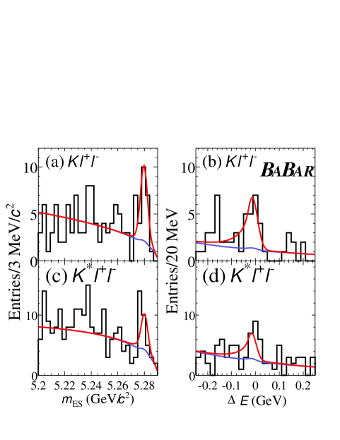
Fig. 12: Projections of $m_{ES}$ and $\Delta E$ for the combined $K^{(*)}\ell^{+}\ell^{-}$ final states. The solid line is the combined signal plus background PDF, the histogram are the data.

5.2 Search for $B^{0}\rightarrow\ell^{+}\ell^{-}$

The decay of a $B$ meson to a pair of leptons is highly suppressed within the SM by factors resulting from CKM, internal quark annihilation and helicity. Leading diagrams are shown in Figure 13. Within the SM, predicted branching fractions are $1.9\times 10^{-15}$ and $8.0\times 10^{-11}$ for the $e^{+}e^{-}$ and $\mu^{+}\mu^{-}$ channels respectively[27]. The $e\mu$ channel is forbidden by lepton number conservation. New physics can significantly alter these predictions[28].

Fig. 13: Leading diagrams for the decay $B\rightarrow\ell^{+}\ell^{-}$.

In this analysis, the primary sources of background are from real lepton production from continuum $c{\bar{c}}$ decays, pions which are mis-identified as muons, and two photon processes. Continuum background is suppressed using the thrust magnitude, and the angle between the thrust axes of the $B$ candidate and the rest of the event. A track multiplicity cut serves to reject two photon processes. The signal is selected by requiring two high momentum leptons of opposite charge and good vertex information. Particle identification requirements for both leptons are made. The signal yield is determined by counting events in a signal region of $m_{ES}$ and $\Delta E$, and subtracting an estimated background determined from the scaled population of the $m_{ES}$ vs $\Delta E$ plane. The results of this analysis applied to a sample of approximately 60 million $B{\bar{B}}$ pairs are presented in Table 3.

	$N_{GSB}$	$N_{SigBox}$	$N_{BG}$	90% CL Upper Limit
${\cal B}(B^{0}\rightarrow e^{+}e^{-})$	25	1	$0.60\pm 0.24$	$3.3\times 10^{-7}$
${\cal B}(B^{0}\rightarrow\mu^{+}\mu^{-})$	26	0	$0.49\pm 0.19$	$2.7\times 10^{-7}$
${\cal B}(B^{0}\rightarrow\mu^{+}\mu^{-})$	26	0	$0.49\pm 0.19$	$2.7\times 10^{-7}$

Table 3: Results of the search for $B\rightarrow\ell^{+}\ell^{-}$. $N_{GSB}$ is the population of the $m_{ES}$ vs $\Delta E$ sideband and $N_{SigBox}$ the population of the signal region after all selection criteria have been applied. $N_{BG}$ is the expected background in the signal region based on the sideband population.

5.3 Search for $B^{+}\rightarrow K^{+}\nu{\bar{\nu}}$

Within the SM, the decay $b\rightarrow s\nu{\bar{\nu}}$ is a pure electroweak flavor changing neutral current. The final state is nearly free of strong interaction uncertainties, and hence the theoretical errors associated with this decay are small. While the inclusive analysis is not currently feasible, it is possible to search for the exclusive decay $B^{+}\rightarrow K^{+}\nu{\bar{\nu}}$. Summing over all neutrino species, the SM prediction for this branching fraction[29] is

$${\cal B}(B^{+}\rightarrow K^{+}\nu{\bar{\nu}})=3.8^{+1.2}_{-0.6}\times 10^{-6}.$$ (13)

The presence of two neutrinos in the final state makes this analysis difficult, as there are no kinematic constraints which may be applied to the signal $B$. Instead, the strategy is to fully reconstruct the other $B$ from the $\Upsilon(4S)$ decay, and compare the remaining particles in the event with the signature expected from the signal. The “tag” $B$ is required to be fully reconstructed as either $B^{-}\rightarrow D^{0}\ell^{-}{\bar{\nu}}$ or $B^{-}\rightarrow D^{*0}\ell^{-}{\bar{\nu}}$. The $D^{0}$ is reconstructed in the $K^{-}\pi^{+}$, $K^{-}\pi^{+}\pi^{-}\pi^{+}$ and $K^{-}\pi^{+}\pi^{0}$ modes, which results in a total of about 0.5% of all charged $B$s being reconstructed as tags. To select signal events, a high momentum charged kaon is required in the recoil of the tagged $B$. Additional requirements are made on the neutral energy in the recoil and on the angle between the kaon and the tag side lepton.

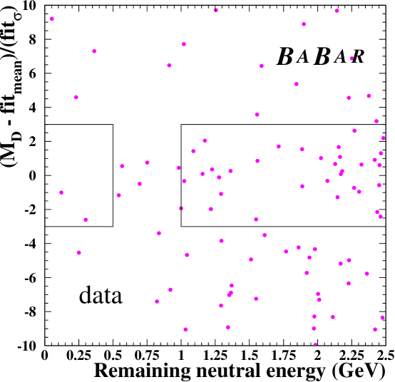
Fig. 14: Distribution of $K^{+}\nu{\bar{\nu}}$ candidates in the plane defined by the electromagnetic energy not from the tag $B$, $E_{Left}$, and the resolution scaled difference between the measured and mean measured $D$ mass. The signal region is the bounded area at the left of the plot.

Events are counted in a signal region in the plane defined by the electromagnetic energy in the tag $B$ recoil, and the difference between the reconstructed and mean fitted $D$ mass, scaled by the fitted $D$ mass resolution. The expected background, determined by scaling the sideband population into the signal region, is subtracted from the signal region population to determine the signal yield. This is illustrated in Figure 14. In a sample of 60 million $B{\bar{B}}$ pairs, the expected background in the signal region is 2.2 events, and there are two events observed. The 90% confidence level upper limit on the branching fraction, including systematics, is

$${\cal B}(B^{+}\rightarrow K^{+}\nu{\bar{\nu}})<9.4\times 10^{-5}.$$ (14)

5.4 Search for $B^{0}\rightarrow\gamma\gamma$

The decay $B^{0}\rightarrow\gamma\gamma$ is an example of electroweak annihilation. The SM expectation for this decay is small, with predictions ranging from 0.1 to $2.3\times 10^{-8}$[30]. As with the other modes discussed in this section, physics beyond the SM can result in significant enhancements to this rate[31].

In this analysis, selection criteria are placed on the ratio of the 2nd to 0th Fox-Wolfram moments, the cosine of the angle between one of the photons (chosen at random) and the thrust axis of the rest of the event, and the $B$ production angle to suppress continuum background. Selected photons are required not to be consistent with having come from a $\pi^{0}$ or $\eta$ decay. The signal yield is determined by counting events in a signal region of the plane defined by $m_{ES}$ and $\Delta E$, and subtracting the expected background determined by scaling the the sideband population into the signal region. The result for a sample of 22 million $B{\bar{B}}$ pairs is

$${\cal B}(B^{0}\rightarrow\gamma\gamma)<1.7\times 10^{-6},$$ (15)

at the 90% confidence level, including systematic uncertainties.

6 Gluonic Penguins (Charmless Hadronic B Decays)

Charmless hadronic $B$ decays proceed through a combination of CKM suppressed tree ($b\rightarrow u$) and gluonic penguin ($b\rightarrow d,s$) amplitudes. There are about 70 possible combinations of two-body decays in the lowest pseudoscalar and vector nonets. These may be further broken into two groups; two-body decays in which both $B$ daughters are kaons or pions, and quasi-two-body decays in which at least one of the $B$ daughters is a short-lived resonance. The two-body modes can be analyzed for information on the CP phases $\alpha$ and $\gamma$, and have been found to have significant penguin contributions in addition to CKM allowed tree amplitudes. Several of the quasi-two-body modes are sensitive to the CP phase $\beta$. In addition to yielding information about the Unitarity Triangle, decays in which penguin amplitudes are dominant are sensitive to new physics. Our study of three-body $B$ decays has thus far been limited to combinations of three charged kaons or pions.

All of these modes share some common features. The primary source of background is random particle combinations in the continuum, although modes with large final state multiplicities or significant neutral energy may suffer from non-negligible $B{\bar{B}}$ backgrounds. All the final states are ultimately composed of high momentum kaons and pions, so the ability to distinguish been these particles at high momenta is crucial.

6.1 Two-Body Decays

Two body $B$ decays to kaons and pions are sensitive to the angle $\alpha$ of the Unitarity Triangle through the time-dependent CP violating asymmetry in the decay $B\rightarrow\pi^{+}\pi^{-}$ and to the the angle $\gamma$ through branching fractions and direct CP-violating asymmetries of decays to various $\pi\pi$ and $K\pi$ final states. Because there are substantial penguin amplitudes which contribute to the $\pi^{+}\pi^{-}$ final state in addition to the tree amplitude, the time-dependent asymmetry in that mode does not directly measure $\alpha$. An isospin analysis of the rates for all the $B\rightarrow\pi\pi$ decays is required to fully unfold the effects of the penguin contributions and determine the relationship between what is measured from the $\pi^{+}\pi^{-}$ analysis ($\alpha_{eff}$) and $\alpha$. Interference between penguin and tree amplitudes may also lead to substantial direct (time-independent) CP asymmetries in the $K\pi$ final states.

In each mode, the signal is extracted using an unbinned extended maximum likelihood fit, using the $m_{ES}$, $\Delta E$, a Fisher discriminant, and where appropriate, Cerenkov angle residuals. Groups of related decays are fit simultaneously. For example, the $\pi^{+}\pi^{-}$, $K^{+}\pi^{-}$ and $K^{+}K^{-}$ yields are determined from a single fit. In these cases, $\Delta E$ and the Cerenkov angle residuals separate the signal modes from each other. Branching fraction results for all two-body modes based on a sample of 88 million $B{\bar{B}}$ pairs can be found in Table 4.

Decay	$N_{Signal}$	${\cal B}\times 10^{-6}$	$A_{CP}$
$B^{0}\rightarrow\pi^{+}\pi^{-}$	$157\pm 19$	$4.7\pm 0.6\pm 0.2$
$B^{0}\rightarrow K^{\pm}\pi^{\mp}$	$589\pm 30$	$17.9\pm 0.9\pm 0.7$	$-0.102\pm 0.050\pm 0.016$
$B^{0}\rightarrow K^{+}K^{-}$	$1\pm 8$	$<0.6$
$B^{+}\rightarrow\pi^{+}\pi^{0}$	$125\pm 22$	$5.5\pm 1.0\pm 0.6$	$-0.03\pm 0.18\pm 0.02$
$B^{+}\rightarrow K^{+}\pi^{0}$	$239\pm 22$	$12.8\pm 1.2\pm 1.0$	$-0.09\pm 0.09\pm 0.01$
$B^{+}\rightarrow K^{0}\pi^{0}$	$86\pm 13$	$10.4\pm 1.5\pm 0.8$	$0.03\pm 0.36\pm 0.09$
$B^{0}\rightarrow\pi^{0}\pi^{0}$	$23\pm 10$	$<3.6\;\;(1.6^{+0.7\;+0.6}_{-0.6\;-0.3})$
$B^{+}\rightarrow K^{0}\pi^{+}$	$172\pm 17$	$17.5\pm 1.8\pm 1.3$	$-0.17\pm 0.10\pm 0.02$
$B^{+}\rightarrow K^{0}K^{+}$	$<10$	$<1.3$

Table 4: Results of two-body branching fraction analyses[9, 10, 11, 12]. The $\pi^{0}\pi^{0}$ result has a statistical significance of $2.5\sigma$. The results for $K^{0}\pi^{+}$ and $K^{0}K^{+}$ are based on 60 million $B{\bar{B}}$ pairs. Upper limits are at the 90% confidence level.

Despite no central measurement of the $\pi^{0}\pi^{0}$ final state, it is still possible to place limits on the relationship between the measured parameter $\alpha_{eff}$ and the Unitarity Triangle parameter $\alpha$. Using the bound of Grossman and Quinn[32] and our measured values, we set an upper limit of $|\alpha_{eff}-\alpha|<51^{\circ}$ at 90% CL.

6.2 Quasi-Two-Body Decays

Quasi-two-body decays proceed through resonant intermediate states. The analysis of such modes is very similar to true two-body decays, but there are additional variables that provide separation between the signal and background, such as the resonance invariant mass and polarization (if the final state is a pseudoscaler-vector combination). We present the analyses of three groups of related quasi-two-body decays; $B\rightarrow\phi K^{(*)}$[13], $B\rightarrow\omega h$[13, 14] and $B\rightarrow\eta^{(\prime)}K^{(*)}$[15].

6.2.1 $B\rightarrow\phi K^{(*)}$

The decay $b\rightarrow s{\bar{s}}s$ is CKM forbidden, thus the decay $B\rightarrow\phi K^{(*)}$ is a nearly pure gluonic penguin, as shown in Figure 15. New physics might not only manifest itself as a deviation from the SM prediction for the decay rate, but since the mode $\phi K^{0}_{S}$ is the strange analog to $J/\psi K^{0}_{S}$, the CP phase one measures in a time-dependent analysis could be altered from it’s SM value of $\beta$.

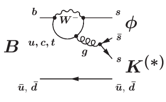
Fig. 15: Leading diagram for the decay $B\rightarrow\phi K^{(*)}$.

The signal yield in each of these modes is determined from an extended unbinned maximum likelihood fit to $m_{ES}$, $\Delta E$, a Fisher discriminant and the $\phi\;(K^{+}K^{-})$ invariant mass. For the $\phi K^{0}_{S}$, $\phi K^{+}$ and $\phi\pi^{+}$ final states, the $\phi$ polarization is included in the fit, as is the Cerenkov angle residual for the charged states. For the $\phi K^{*}$ final states, the $K^{*}$ invariant mass is included in the fit. Significant signals are observed for both charged and neutral $B$ decays to $K$ and $K^{*}$ final states. The results of this analysis on a sample of 60 million $B{\bar{B}}$ pairs are

$${\cal B}(B^{+}\rightarrow\phi K^{+}) = (9.2\pm 1.0\pm 0.8)\times 10^{-6}$$

$${\cal B}(B^{+}\rightarrow\phi K^{0}) = (8.7^{+1.7}_{-1.5}\pm 0.9)\times 10^{-6}$$

$${\cal B}(B^{+}\rightarrow\phi K^{*+}) = (9.7^{+4.2}_{-3.4}\pm 1.7)\times 10^{-6}$$

$${\cal B}(B^{+}\rightarrow\phi K^{*0}) = (8.7^{+2.5}_{-2.1}\pm 1.1)\times 10^{-6}$$

$${\cal B}(B^{+}\rightarrow\phi\pi^{+}) < 0.56\times 10^{-6}\;@\;90\%\;{\rm CL}.$$ (16)

A stringent limit is also placed on the decay $B^{+}\rightarrow\phi\pi^{+}$, which is both CKM and color suppressed.

6.2.2 $B\rightarrow\omega h\;(h=K,\pi)$

$B$ decays involving an omega and either a kaon or a pion proceed through a mixture of CKM suppressed $b\rightarrow u$ tree and CKM forbidden $b\rightarrow d,s$ penguin amplitudes. The analysis method is identical to that described for $\phi K^{(*)}$. The results in Table 5 are based on a sample of 22 million $B{\bar{B}}$, except for the $\omega K^{0}_{S}$ analysis, which was performed on a sample of 60 million $B{\bar{B}}$ pairs, and is a first observation.

Final State	$N_{Signal}$	$S(\sigma)$	${\cal B}\times 10^{-6}$
$\omega K^{+}$	$6.4^{+5.6}_{-4.4}$	1.3	$<4\;(1.4^{+1.3}_{-1.0}\pm 0.3)$
$\omega K^{0}$	$26.6^{+7.7}_{-6.6}$	6.6	$5.9^{+1.7}_{-1.5}\pm 0.9$
$\omega\pi^{+}$	$27.6^{+8.8}_{-7.7}$	4.9	$6.6^{+2.1}_{-1.8}\pm 0.7$
$\omega\pi^{0}$	$-0.9^{+5.0}_{-3.2}$	-	$<3\;(-0.3\pm 1.1\pm 0.3)$

Table 5: Results of the branching fraction analysis of $B\rightarrow\omega h$. S is the statistic significance of the result. Upper limits are at the 90% confidence level.

6.2.3 $B\rightarrow\eta^{(\prime)}K^{(*)}$

$B$ decays to $\eta$ and $\eta^{\prime}$ with a kaon or $K^{*}$ proceed predominantly through penguins, although there is some $b\rightarrow u$ tree contribution as well. The decays $B\rightarrow\eta^{\prime}K$ and $B\rightarrow\eta K^{*}$ were the first gluonic penguins to be observed[33], and the rates are much larger than initially expected. The best present conjecture[34] is that the tree and penguin amplitudes interfere in such a way as to enhance $\eta^{\prime}K$ and $\eta K^{*}$ but suppress $\eta^{\prime}K^{*}$ and $\eta K$. Because of it’s relatively large rate and nearly pure penguin content, $B\rightarrow\eta^{\prime}K^{0}_{S}$ is also of considerable interest for measurements of time-dependent CP asymmetries, which within the SM should probe the angle $\beta$.

Signals for these modes are extracted as described above for $\omega$ and $\phi$. The $\eta^{\prime}$ is reconstructed in two decay chains; $\eta(\gamma\gamma)\pi^{+}\pi^{-}$ and $\rho^{0}\gamma$. The $\eta$ is reconstructed as $\eta\rightarrow\gamma\gamma$ and $\eta\rightarrow\pi^{+}\pi^{-}\pi^{0}$. The results of these analyses are displayed in Table 6. The data samples used for the $\eta$ and $\eta^{\prime}$ analyses are 22 and 60 million $B{\bar{B}}$ pairs respectively.

Final State	$N_{Signal}$	${\cal B}\times 10^{-6}$
$\eta^{\prime}K^{+}$	$445\pm 26$	$67\pm 5\pm 5$
$\eta^{\prime}K^{0}$	$135\pm 15$	$46\pm 6\pm 4$
$\eta^{\prime}K^{*0}$	$5.2\pm 3.4$	$<13\;(4.0^{+3.5}_{-2.4}\pm 1.0)$
$\eta K^{+}$	$12.9\pm 5.7$	$<6.4\;(3.8^{+1.8}_{-1.5}\pm 0.2)$
$\eta\pi^{+}$	$8.0\pm 5.9$	$<5.2\;(2.2^{+1.8}_{-1.6}\pm 0.1)$
$\eta K^{0}$	$5.7\pm 3.3$	$<12\;(6.0^{+3.8}_{-2.9}\pm 0.4)$
$\eta K^{*0}$	$20.5\pm 6.3$	$19.8^{+6.5}_{-5.6}\pm 1.5$
$\eta K^{*+}$	$14.3\pm 6.6$	$22.1^{+11.1}_{-9.2}\pm 3.2$

Table 6: Results of the branching fraction analyses of $B\rightarrow\eta^{(\prime)}K^{(*)}$. Upper limits are at the 90% confidence level.

6.3 Three-Body Decays

We describe here the analysis of $B^{+}\rightarrow h^{+}h^{-}h^{+}$[16], where $h$ is either a charged kaon or pion. An event counting analysis is performed over the full three particle dalitz plot. All final states are measured simultaneously, and unfolded to obtain branching fractions for each combination. Continuum background is suppressed using the thrust angle and a Fisher discriminant. In addition to continuum background, the open nature of the dalitz plot also admits background in some regions from $B^{+}\rightarrow J/\Psi K^{+}$ and $B^{+}\rightarrow D\pi^{+}/DK^{+}$. These regions of the dalitz plot are vetoed. Charged particle identification is crucial to this analysis, and along with tracking, is the primary source of systematic uncertainty. Figure 16 shows the dalitz plots for $B^{+}\rightarrow K^{+}K^{-}K^{+}$ and $B^{+}\rightarrow K^{+}\pi^{-}\pi^{+}$. Results of this analysis on a sample of 56 million $B{\bar{B}}$ pairs are

$${\cal B}(B^{\pm}\rightarrow\pi^{\pm}\pi^{\mp}\pi^{\pm}) < 15\times 10^{-6}\;@\;90\%\;{\rm CL}\;(8.5\pm 4.0\pm 3.6)$$

$${\cal B}(B^{\pm}\rightarrow K^{\pm}\pi^{\mp}\pi^{\pm}) = (59.2\pm 4.7(stat)\pm 4.9(sys))\times 10^{-6}$$

$${\cal B}(B^{\pm}\rightarrow K^{\pm}K^{\mp}\pi^{\pm}) < 7\times 10^{-6}\;@\;90\%\;{\rm CL}\;(2.1\pm 2.9\pm 2.0)$$

$${\cal B}(B^{\pm}\rightarrow K^{\pm}K^{\mp}K^{\pm}) = (34.7\pm 2.0(stat)\pm 1.8(sys))\times 10^{-6}.$$ (17)

Fig. 16: Unbinned dalitz plots for $K^{+}\pi^{-}\pi^{+}$ (left) and $K^{+}K^{-}K^{+}$ (right) for events in the signal region. No efficiency corrections have been applied to the dalitz plots, and the charm contributions have not been removed.

7 Conclusion and Outlook

We have presented a number of results for rare $B$ meson decays using all or part of a sample of approximately 88 million $B{\bar{B}}$ pairs collected by the BABAR detector. Updates of many of these analyses to the full data set are in progress. These results represent only a part of the spectrum of possible measurements of rare decays. The larger data sets that will be available in the coming years will allow us to more fully exploit rare decays to test the self consistency of the flavor sector of the Standard Model, and will perhaps offer the first glimpse of new physics which lies beyond.

8 Acknowledgments

We are grateful for the excellent luminosity and machine conditions provided by our PEP-II colleagues, and for the substantial dedicated effort from the computing organizations that support BABAR. The author’s work was performed under the auspices of the U.S. Department of Energy by the University of Colorado under Contract DE-FG03-95ER40894.

References

- [1] B. Aubert et al. [BABAR Collaboration], Phys. Rev. Lett. 88, 101805 (2002) [arXiv:hep-ex/0110065].
- [2] B. Aubert et al. [BABAR Collaboration], arXiv:hep-ex/0207073.
- [3] B. Aubert et al. [BABAR Collaboration], arXiv:hep-ex/0207074.
- [4] B. Aubert et al. [BABAR Collaboration], arXiv:hep-ex/0207076.
- [5] B. Aubert et al. [BABAR Collaboration], arXiv:hep-ex/0207082.
- [6] B. Aubert et al. [BABAR Collaboration], arXiv:hep-ex/0207083.
- [7] B. Aubert et al. [BABAR Collaboration], arXiv:hep-ex/0207069.
- [8] B. Aubert et al. [BABAR Collaboration], Phys. Rev. Lett. 87, 241803 (2001) [arXiv:hep-ex/0107068].
- [9] B. Aubert et al. [BABAR Collaboration], Phys. Rev. Lett. 89, 281802 (2002) [arXiv:hep-ex/0207055].
- [10] B. Aubert et al. [BABAR Collaboration], arXiv:hep-ex/0207065.
- [11] B. Aubert et al. [BABAR Collaboration], arXiv:hep-ex/0207053.
- [12] B. Aubert et al. [BABAR Collaboration], arXiv:hep-ex/0207063.
- [13] A. Bevan, to appear in Proceedings of the 31st International Conference on High Energy Physics.
- [14] B. Aubert et al. [BABAR Collaboration], Phys. Rev. Lett. 87, 221802 (2001) [arXiv:hep-ex/0108017].
-
[15]
P. Bloom, “Branching Fractions for ”,
2002 Meeting of the APS Division of Particles and Fields, May 24, 2002.
http://dpf2002.velopers.net/talks_pdf/361talk.pdf - [16] B. Aubert et al. [BABAR Collaboration], arXiv:hep-ex/0206004.
- [17] B. Aubert et al. [BABAR Collaboration], Nucl. Instrum. Meth. A 479, 1 (2002) [arXiv:hep-ex/0105044].
- [18] N. Cabibbo, Phys. Rev. Lett. 10, 531 (1963). M. Kobayashi and T. Maskawa, Prog. Theor. Phys. 49, 652 (1973).
- [19] H. Albrecht et al. [ARGUS Collaboration], Phys. Lett. B 241, 278 (1990).
- [20] T. E. Coan et al. [CLEO Collaboration], Phys. Rev. Lett. 84, 5283 (2000) [arXiv:hep-ex/9912057].
- [21] Except as noted explicitly, we use a particle name to denote either member of a charge conjugate pair.
- [22] S. W. Bosch and G. Buchalla, Nucl. Phys. B 621, 459 (2002) [arXiv:hep-ph/0106081].
- [23] M. Beneke, T. Feldmann and D. Seidel, Nucl. Phys. B 612, 25 (2001) [arXiv:hep-ph/0106067].
- [24] A. Ali and A. Y. Parkhomenko, Eur. Phys. J. C 23, 89 (2002) [arXiv:hep-ph/0105302].
- [25] A. L. Kagan and M. Neubert, Eur. Phys. J. C 7, 5 (1999) [arXiv:hep-ph/9805303].
- [26] A. Ali, P. Ball, L. T. Handoko and G. Hiller, Phys. Rev. D 61, 074024 (2000) [arXiv:hep-ph/9910221].
- [27] A. Ali, C. Greub and T. Mannel, DESY-93-016 To be publ. in Proc. of ECFA Workshop on the Physics of a B Meson Factory, Eds. R. Aleksan, A. Ali, 1993
- [28] M. Gronau and D. London, Phys. Rev. D 55, 2845 (1997) [arXiv:hep-ph/9608430].
- [29] P. F. Harrison and H. R. Quinn [BABAR Collaboration], SLAC-R-0504 Papers from Workshop on Physics at an Asymmetric B Factory (BaBar Collaboration Meeting), Rome, Italy, 11-14 Nov 1996, Princeton, NJ, 17-20 Mar 1997, Orsay, France, 16-19 Jun 1997 and Pasadena, CA, 22-24 Sep 1997
- [30] G. G. Devidze and G. R. Dzhibuti, Phys. Lett. B 429, 48 (1998).
- [31] T. M. Aliev and G. Turan, Phys. Rev. D 48, 1176 (1993).
- [32] Y. Grossman and H. R. Quinn, Phys. Rev. D 58, 017504 (1998) [arXiv:hep-ph/9712306].
- [33] S. J. Richichi et al. [CLEO Collaboration], Phys. Rev. Lett. 85, 520 (2000) [arXiv:hep-ex/9912059].
- [34] M. Beneke and M. Neubert, Nucl. Phys. B 651, 225 (2003) [arXiv:hep-ph/0210085].