Measurements of Charmless Hadronic Two-Body B Meson Decays and the Ratio $\mbox{${\cal B}$}(B\to DK)/\mbox{${\cal B}$}(B\to D\pi)$

Abstract

We present final measurements of thirteen charmless hadronic $B$ decay modes from the CLEO experiment. The decay modes include the ten $\pi\pi$, $K\pi$, and KK final states and new limits on dibaryonic final states, ${p\bar{p}}$, ${p\bar{\Lambda}}$, and ${\Lambda\bar{\Lambda}}$, as well as a new determination of the ratio $\mbox{${\cal B}$}(B\to DK)/\mbox{${\cal B}$}(B\to D\pi)$. The results are based on the full CLEO II and CLEO III data samples totalling 15.3 ${\rm fb}^{-1}$ at the $\Upsilon(4S)$, and supercede previously published results.

I Introduction

Charmless decays of $B$ mesons may proceed by $b\to u$, $b\to s$, or $b\to d$ transitions. The latter two mechanisms require flavor changing neutral currents which are not present at tree level in the Standard Model, and therefore must occur through higher order processes such as the penguin mechanism. Such processes involve loops, which can open the window for particles and physics outside the Standard Model. Even in the absence of such new physics, interference among competing amplitudes for a given decay mode can be exploited to measure CKM phases. There is a significant body of literaturefleischeretal on the use of the branching ratio $\mbox{${\cal B}$}(B\to K^{-}\pi^{+})$ and other charmless modes to determine or constrain the CKM angle $\gamma$, the phase of $V_{ub}$ in conventional representations of the CKM matrix. Compared to the methods of extracting $\gamma$ that are based the $B\to DK$ decay modesDK , these approaches based on charmless decay modes are less clean theoretically, but more promising experimentally because the event yields are significantly higher.

Recent work on two-body charmless decay modes suggests that the unitarity triangle may be constructable entirely from charmless modes, without recourse to the traditional constraints involving $B$ mixing measurements, CP asymmetry in $B\to J/\psi\mbox{$K^{0}_{S}$}$, or CP violation in kaon decays. The charmless modes therefore offer an independent approach to probe CP violating effects in heavy quark decay. Significant disagreement between these two approaches, if found in experimental results, would directly challenge the Standard Model and its fundamental statement that all CP violating phenomena stem from a single phase in the CKM matrix. Early results based on current data are already availableneubertnew , and do indicate a degree of inconsistency. In this paper we present new experimental data on charmless modes and note that these data enhance rather than ameliorate the discrepancy.

CLEO has previously published several papersprevious reporting measurements of charmless hadronic $B$ meson decay modes, including searches for charmless baryonic final states, with the data of the CLEO II experiment. Here we report corresponding measurements in the new CLEO III data with results for three $\pi\pi$ modes, $B\to\pi^{+}\pi^{-},~{}\pi^{+}\pi^{0},~{}\mbox{$\pi^{0}$}\mbox{$\pi^{0}$}$, four $K\pi$ modes, $B\to K^{+}\pi^{-},~{}K^{+}\pi^{0},~{}\mbox{$K^{0}$}\pi^{+},~{}\mbox{$K^{0}$}\pi^{0}$, three $K\overline{K}$ modes, $B\to K^{+}K^{-},~{}\mbox{$K^{0}$}K^{-},~{}\mbox{$K^{0}$}\mbox{$\overline{K^{0}}$}$, and three dibaryonic modes, $B\to\mbox{${p\bar{p}}$},~{}\mbox{${p\bar{\Lambda}}$},~{}\mbox{${\Lambda\bar{\Lambda}}$}$. We also merge CLEO II and CLEO III results to determine a final measurement for each mode based on the full CLEO data set, which hereby supercedes our previous publications. Recent measurements from BABAR and Belle are in excellent agreement with oursbabarandbelle . We also report a new measurement of the ratio of branching ratios, $\mbox{${\cal B}$}(B\to D^{0}K^{-})/\mbox{${\cal B}$}(B\to D^{0}\pi^{-})$.

Here and throughout this paper charge conjugate modes are implied. We also make use of the notation $h^{\pm}$ to represent a charged hadron that may be either a kaon or pion.

II The CLEO Detector and Datasets

CLEO is a general purpose solenoidal magnet detector operating at the Cornell Electron Storage Ring (CESR). The latter is a symmetric-energy storage ring tuned for the data sets discussed here to provide center of mass energies near the $\Upsilon$(4S). At $\sqrt{s}=M_{\mbox{$\Upsilon$({\rm 4S})}}$ the hadronic cross section is approximately 4 nb, with 1 nb of $\mbox{$e^{+}e^{-}$}\to\mbox{$\Upsilon$({\rm 4S})}\to\mbox{$B\bar{B}$}$ and 3 nb of four-flavor continuum $e^{+}e^{-}\to\mbox{$q\bar{q}$}$. In the CLEO III running period, July 2000 through June 2001, we obtained an integrated luminosity of 6.18 ${\rm fb}^{-1}$ at the $\Upsilon$(4S) and 2.24 ${\rm fb}^{-1}$ off-resonance, i.e., just below the $B\bar{B}$ threshold. The off-resonance data are used for background determinations. The on-resonance data corresponds to $\mbox{$N_{B\bar{B}}$}=(5.73\pm 0.47)\mbox{${\times 10^{6}}$}$ $\Upsilon$(4S) decays. The corresponding numbers for the CLEO II running period (1990-1999) are 9.13 ${\rm fb}^{-1}$ (($9.66\pm 0.19)\mbox{${\times 10^{6}}$}$$\Upsilon$(4S) decays) and 4.35 ${\rm fb}^{-1}$. Differences in the $N_{B\bar{B}}$ yield per unit integrated luminosity reflect differences in run conditions.

The CLEO III detectorcleo3det differs from the CLEO II detectorcleo2det most notably in the inclusion of a ring-imaging Cherenkov device (RICH)rich which provides particle identification at all momenta above the Cherenkov threshold. Even at the highest momenta relevant for $B$ physics, about 2.8 ${\rm~{}GeV}$, the RICH separates kaons and pions by 2.3 standard deviations. Measurements of specific ionization ($dE/dx$) in the drift chamber provide an additional 2.0 standard deviation separation at the highest momenta. Charged particle tracking is done by the 47-layer drift chamber and a four-layer silicon tracker which reside in a 1.5T solenoidal magnetic field and provide momentum resolution described by $(\sigma_{p}/p)^{2}=A^{2}+B^{2}p^{2}$ with $A\approx 0.005$ and $B\approx 0.001~{}\mbox{${\rm~{}GeV}$}^{-1}$. The absolute momentum calibration is confirmed by comparing the invariant mass of standard decays $J/\psi\to\mu^{+}\mu^{-}$, $D^{0}\to K^{-}\pi^{+}$ with PDG valuespdg . Photons are detected using a 7800-crystal CsI(Tl) electromagnetic calorimeterwhich is unchanged between CLEO II and CLEO III.

III Elements of the analysis

The $\Upsilon$(4S) is produced at rest in the lab frame and decays with low $Q$ value to a pair of $B$ mesons that travel non-relativistically, with $\mbox{$p_{B}$}\sim 300~{}\mbox{${\rm MeV}$}$. In this analysis we assume equal rates of $B^{+}B^{-}$ and $B^{0}\bar{B^{0}}$ productionfplusminuscleo . All decay modes studied in this paper are two-body or quasi-two-body modes. Apart from the modest $\pm 150~{}\mbox{${\rm MeV}$}$ doppler shifts resulting from the motion of the $B$ mesons in the lab frame, the daughter particles are nearly monochromatic, and, up to resolution smearing, jointly carry the full beam energy $E_{b}$ and have invariant mass equal to the $B$ mass $M_{B}$. The approximate monochromaticity of the daughters simplifies particle identification and energy resolution, and helps keep the associated systematic errors low. The other $B$ in the event decays into, on average, five charged and five neutral particles, distributed uniformly in the detector acceptance. The principal background to the analysis comes from the non-$b$ hadronic data, $e^{+}e^{-}\to\mbox{$q\bar{q}$}$, with $\mbox{${q\bar{q}}$}=u\bar{u},~{}d\bar{d},~{}s\bar{s},~{}{\rm and}~{}c\bar{c}.$ High momentum, back-to-back particles are typical in such events, and some have invariant masses and total energies close to or in the signal region of the $B$ events. Fortunately, distinctive event topologies separate most of these background events from the signal.

This analysis has two principal parts: (a) the application of hard selection criteria to obtain signal-like events, based on kinematics, event topology, and particle identification; (b) the application of an unbinned extended maximum likelihood fit to the surviving event ensembles to extract the yields of signal and background(s) for each mode. The likelihood fit allows us to make maximum use of available information, while avoiding efficiency losses that further selection criteria would entail.

For the purposes of reconstruction, the CLEO III dataset reported on here is divided into two subsets of roughly equal integrated luminosity, which we will call Set A and Set B. The distinction has ultimately no significant effect on the results, but because of changes in event reconstruction algorithms between the two sets, there are slight differences in resolutions and efficiencies – mostly affecting modes with charged particles – that we treat separately until the final CLEO III results are reassembled at the end. We provide in Table 1 some informative comparisons between Set A and Set B.

Table 1: Features of Set A and Set B.

Quantity	Set A	Set B
Fraction of total $N_{B\bar{B}}$	55%	45%
Track Resolution
‘A’ Coefficient	0.0055	0.0044
‘B’ Coefficient ($\mbox{${\rm~{}GeV}$}^{-1}$)	0.0011	0.0010
$K^{+}\pi^{-}$ Mode
$\sigma_{\mbox{$M_{B}$}}$ (${\rm MeV}$)	2.7	2.7
$\sigma_{\mbox{$\Delta E$}}$(${\rm MeV}$)	22	19
Efficiency	38%	45%
$K^{+}\pi^{0}$ Mode
$\sigma_{\mbox{$M_{B}$}}$ (${\rm MeV}$)	3.1	3.1
$\sigma_{\mbox{$\Delta E$}}$(${\rm MeV}$)	31	31
Efficiency	33%	35%
$\pi^{0}\pi^{0}$ Mode
$\sigma_{\mbox{$M_{B}$}}$ (${\rm MeV}$)	3.6	3.6
$\sigma_{\mbox{$\Delta E$}}$(${\rm MeV}$)	43	43
Efficiency	22%	22%

Charged track and photon candidates are required to satisfy loose quality requirements which reject poorly determined candidates while retaining high efficiency for real tracks and showers. $K^{0}_{S}$ candidates are selected from pairs of charged tracks forming well-measured displaced vertices with a $\pi^{+}\pi^{-}$ invariant mass within three standard deviations of the nominal $K^{0}_{S}$ mass. In addition the vertex must satisfy $|r_{VTX}|>5$mm in the transverse plane, and ${\vec{p}_{\mbox{$K^{0}_{S}$}}}\cdot{\vec{r}_{VTX}}>0$. The $\mbox{$K^{0}_{S}$}\to\mbox{$\pi^{0}$}\mbox{$\pi^{0}$}$ mode is not used. $\Lambda$ candidates consist of $p\pi$ pairs with invariant mass within three standard deviations of the nominal $\Lambda$ mass. Pairs of photons with an invariant mass within 2.5 standard deviations of the nominal $\pi^{0}$ mass are kinematically fit with the mass constrained to the nominal $\pi^{0}$ mass.

III.1 General Event Selection

Candidates for rare $B$ decay events are selected for further analysis on the basis of two kinematic variables and one event-shape variable. For each candidate, we construct the beam constrained $B$ candidate mass $M_{B}=\sqrt{(E_{b}^{2}-{\vec{p}}^{~{}2})}$ where $E_{b}$ is the beam energy, and $\vec{p}$ is the momentum of the candidate computed from the vector sum of the daughter momenta. For real $B$ mesons $|\vec{p}|\ll E_{b}$ and the width of this distribution is dominated by the $\sim 2.5~{}\mbox{${\rm MeV}$}$ intrinsic beam energy spread. The beam energy is determined run by run from CESR lattice information, and slight corrections are applied afterward to ensure that the observed $B^{-}$ mass in $B^{-}\to D^{0}\pi^{-}$ events matches the accepted valuepdg . In addition we compute the energy balance variable $\Delta E$ = $E-E_{b}$ where $E$ is the sum of the daughter energies. The width of this distribution is about 20 ${\rm MeV}$ in all charged modes, as determined by the momentum resolution of the tracking systems, and is about 40 ${\rm MeV}$ in modes involving neutral pions.

Any candidate with $|\Delta E|<400$ MeV and $M_{B}>5.2$ GeV is kept. An additional requirement on $\cos\theta_{\rm sph}$, the cosine of the angle between the sphericity axis of the candidate and the sphericity axis of the rest of the eventprevious , is used to reject the dominant $e^{+}e^{-}\to\mbox{$q\bar{q}$}$ background. All candidates must satisfy the requirement $|\mbox{$\cos\theta_{\rm sph}$}|<0.8$, which rejects approximately 80% of the background while retaining nearly 80% of the signal.

III.2 Particle Identification Requirements (CLEO III)

In the case of a candidate mode involving one or more charged pions or kaons, such as $B\to\mbox{$K\pi$}$ or $B\to\pi\mbox{$\pi^{0}$}$, each charged track must be positively identified as $K$ or $\pi$. The pattern of Cherenkov photon hits in the RICH detector is fit to both a kaon and pion hypothesis, each with its own likelihood $\mbox{${\cal L}$}_{K}$ and $\mbox{${\cal L}$}_{\pi}$. The mean number of photon hits entering the fit is twelve, and we require a minimum of four. Calibrated $dE/dx$ information from the drift chamber is used to compute a $\chi^{2}$ for kaon and pion hypotheses. The RICH and $dE/dx$ results are combined to form an effective $\chi^{2}$ difference,

$$\mbox{$\Delta_{K\pi}$}=-2\ln\mbox{${\cal L}$}_{K}+2\ln\mbox{${\cal L}$}_{\pi}+\mbox{$\chi^{2}$}_{K}-\mbox{$\chi^{2}$}_{\pi}.$$ (1)

Kaons are identified by $\mbox{$\Delta_{K\pi}$}<\delta_{K}$ and pions by $-\mbox{$\Delta_{K\pi}$}<\delta_{\pi}$, with values of $\delta_{K}$ and $\delta_{\pi}$ chosen to yield $(90\pm 3)$% efficiency as determined in an independent study of tagged kaons and pions obtained from the decay $D^{*+}\to\pi^{+}D^{0}~{}(D^{0}\to K^{-}\pi^{+})$. With this choice of $\delta_{K}$ and $\delta_{\pi}$, the misidentification rate for kaons faking pions (pions faking kaons) is 11%(8%) at momenta around 2.6 ${\rm~{}GeV}$.

For candidate modes involving protons, positive proton identification is required. $dE/dx$ does not distinguish well between protons and kaons at the $\sim 2.5~{}\mbox{${\rm~{}GeV}$}$ momenta of interest, however, so the proton-kaon separation is achieved with a discriminant based only on RICH information: $\mbox{$\Delta_{Kp}$}=-2\ln\mbox{${\cal L}$}_{p}+2\ln\mbox{${\cal L}$}_{K}<\delta_{p}$. In this case $\delta_{p}$ is chosen to yield proton (antiproton) identification efficiency of $76\pm 1(72\pm 1)$% with a kaon fake rate of 1%, as determined in an independent study using tagged kaons from the $D^{*+}$ sample as above, and protons from $\Lambda\to p\pi$ decays.

III.3 Event Selection for CLEO II modes

We present three results for which we also analyzed the full CLEO II data set, namely $B\rightarrow\mbox{$K^{0}$}\mbox{$\overline{K^{0}}$}$, $B\rightarrow\Lambda\overline{\Lambda}$, and $B\rightarrow p\overline{\Lambda}$. The $K^{0}_{S}$ selection required that the $K^{0}_{S}$ vertex is separated from the beam spot by more that 3 sigma (5.5 sigma for CLEO II.V for which the innermost drift chamber was replaced with a 3 layer silicon vertex detector). The candidate mass must lie within 10 MeV of the nominal $K^{0}_{S}$ mass. We require that the $K^{0}_{S}$ flight direction points to within 3 sigma of the beamspot .

The protons in the ${p\bar{\Lambda}}$ final state must be compatible within 3 sigma with a proton $dE/dx$ hypothesis and incompatible with both the electron (calculated from calorimeter information) and muon (calculated from muon chamber information) hypotheses. We require that the $\Lambda$ candidate mass lie within 10 MeV of the nominal $\Lambda$ mass, the vertex be at least 5 mm removed radially from the beam spot, and the $\chi^{2}$ of the vertex fit be less than nine. There is no particle identification applied to daughter particles of the $\Lambda$ decays.

IV Analysis Variables

Events which meet all the requirements described in the preceding paragraphs are now used in a likelihood fit to extract signal yield. We characterize each candidate event by four variables: the mass and energy variables introduced above, $M_{B}$ and $\Delta E$, the flight direction of the candidate $B$, and a Fisher discriminantFisher .

The flight direction is given by $\mbox{${\cos\theta_{\rm B}}$}=\hat{\bf p}\cdot\mbox{$\hat{\bf z}$}$ where ${\bf p}$ is the vector sum of the daughter momenta and $\hat{\bf z}$ is the beam axis. Since the vector $\Upsilon$(4S) is produced in $e^{+}e^{-}$ annihilation it has a polarization $J_{z}=\pm 1$, and the subsequent flight direction of the pseudoscalar $B$ mesons is distributed as $|Y^{\pm 1}_{1}(\theta,\phi)|^{2}\sim\sin^{2}\theta=1-\cos^{2}\theta$. Background events are flat in this variable.

The Fisher discriminant is used to refine the separation of signal and $e^{+}e^{-}\to\mbox{$q\bar{q}$}$ background that is initially addressed by the hard cut on $\cos\theta_{\rm sph}$ in the general event selection. The Fisher discriminant, $x_{\cal F}$, is a linear combination of fourteen variables, with coefficients chosen to maximize the separation of signal and background events. The optimization procedure uses Monte Carlo events for the signal and off-resonance and ($M_{B}$,$\Delta E$) sideband data events for the background. As in previous CLEO publicationsprevious the component variables include the direction of the thrust axis of the candidate with respect to the beam axis, $\cos\theta_{\rm thr}$, and the nine conical bins of a “Virtual Calorimeter” whose axis is aligned with the candidate thrust axis. A fuller description of the Virtual Calorimeter is available in a previous publicationbigrareb . Note that $\cos\theta_{\rm thr}$ and ${\cos\theta_{\rm B}}$ are quite different quantities. For two body decay $B\to XY$, one has simple closed form expressions: $\mbox{${\cos\theta_{\rm B}}$}=\hat{\bf p}\cdot\mbox{$\hat{\bf z}$}$ with ${\bf p}\equiv{\bf p}_{X}+{\bf p}_{Y}$, whereas $\mbox{$\cos\theta_{\rm thr}$}=\hat{\bf q}\cdot\mbox{$\hat{\bf z}$}$ with ${\bf q}\equiv{\bf p}_{X}-{\bf p}_{Y}$.

In addition, we take advantage of the high quality particle identification in CLEO III to augment the Fisher discriminant with information on the presence of electrons, muons, protons, and kaons in the event. The momentum of the highest momentum electron, muon, kaon, and proton are used as inputs to the Fisher discriminant. For these purposes we need only rudimentary particle identification criteria. If any of the possible particle type hypotheses has no corresponding track identified (which is very often the case), a value zero is used as the input to the Fisher discriminant.

The Fisher variable thus defined provides discrimination between charmless $B$ decay signal modes and ${q\bar{q}}$ background at a level equivalent to two gaussian distributions separated by 1.4$\sigma$, and is independent of the details of the signal mode for all the modes studied here.

V Likelihood Fit

V.1 Fit Components

With the four analysis variables $M_{B}$, $\Delta E$, $x_{\cal F}$, and ${\cos\theta_{\rm B}}$, we characterize each event in terms of normalized probability distribution functions (${PDF}{\rm s}$): $\mbox{${\cal M}$}\mbox{${}_{\mbox{${\mu}$}\mbox{${\kappa}$}}$}(\mbox{$M_{B}$})$, $\mbox{${\cal E}$}\mbox{${}_{\mbox{${\mu}$}\mbox{${\kappa}$}}$}(\mbox{$\Delta E$})$, $\mbox{${\cal F}$}\mbox{${}_{\mbox{${\mu}$}\mbox{${\kappa}$}}$}(\mbox{$x_{\cal F}$})$, and $\mbox{${\cal C}$}\mbox{${}_{\mbox{${\mu}$}\mbox{${\kappa}$}}$}(\mbox{${\cos\theta_{\rm B}}$})$. The thirteen different charmless decay modes to be fit will in general have contributions from (a) signal, (b) ${q\bar{q}}$ background, and (c) cross-feed from other $B$ modes. Subscripts ${\mu}$ and ${\kappa}$ identify the particular decay mode (${\mu}$) and the type of contribution (${\kappa}$). The probability that a given event characterized by ($M_{B}$, $\Delta E$, $x_{\cal F}$, ${\cos\theta_{\rm B}}$) is an event of component type ${\kappa}$ of decay mode ${\mu}$ is then given by the product of ${PDF}{\rm s}$

$$P\mbox{${}_{\mbox{${\mu}$}\mbox{${\kappa}$}}$}=\mbox{${\cal M}$}\mbox{${}_{\mbox{${\mu}$}\mbox{${\kappa}$}}$}(\mbox{$M_{B}$})\mbox{${\cal E}$}\mbox{${}_{\mbox{${\mu}$}\mbox{${\kappa}$}}$}(\mbox{$\Delta E$})\mbox{${\cal F}$}\mbox{${}_{\mbox{${\mu}$}\mbox{${\kappa}$}}$}(\mbox{$x_{\cal F}$})\mbox{${\cal C}$}\mbox{${}_{\mbox{${\mu}$}\mbox{${\kappa}$}}$}(\mbox{${\cos\theta_{\rm B}}$}).$$ (2)

We determine the yields ${n}_{\mbox{${\kappa}$}}$ of signal, ${q\bar{q}}$ background, and cross-feed background in decay mode ${\mu}$ by maximizing the extended likelihood function with respect to the yields ${n}_{\mbox{${\kappa}$}}$:

$$\mbox{${\cal L}$}_{\mbox{${\mu}$}}(n_{sig},n_{\mbox{${q\bar{q}}$}},n_{xfeed})={\exp(-{\sum_{\mbox{${\kappa}$}}{\mbox{${n}_{\mbox{${\kappa}$}}$}}})\prod_{\rm events}{\left(\sum_{\mbox{${\kappa}$}}{\mbox{${n}_{\mbox{${\kappa}$}}$}P\mbox{${}_{\mbox{${\mu}$}\mbox{${\kappa}$}}$}}\right)}.}$$ (3)

The ${q\bar{q}}$ background is the dominant background source in all cases, and in only five of the fifteen modes do we need to include any cross-feed backgrounds. Four of these are due to the $\sim 10\%$ $K/\pi$ misidentification probability. In fitting $B\to\pi^{+}\pi^{-}$ and $B\to\pi^{+}\pi^{0}$ we include components for $B\to K^{+}\pi^{-}$ and $B\to K^{+}\pi^{0}$, respectively; in $B\to K^{+}K^{-}$ we include a component for $B\to K^{+}\pi^{-}$; and in $B\to D^{0}K^{-}$ we include a component for $B\to D^{0}\pi^{-}$. Although the cross-feed backgrounds arise from mistaken particle identification, they are still distinguishable from the signal through $\mbox{${\cal E}$}(\mbox{$\Delta E$})$, which is shifted by about 50 ${\rm MeV}$ relative to the signal ${PDF}$. The cross-feed fits are only for background removal and the yields are not used in any other signal determination.

The fifth mode requiring a cross-feed component is $B^{0}\to\mbox{$\pi^{0}$}\mbox{$\pi^{0}$}$. In this case a small contribution from $B^{+}\to\rho^{+}\pi^{0}$ arises when the charged pion has very little momentum in the lab frame. Although the missing particle also shifts $\Delta E$ by at least one pion mass, resolution smearing leaves a small tail in the signal region. The treatment here is the same as in our previous publication on $B^{0}\to\mbox{$\pi^{0}$}\mbox{$\pi^{0}$}$previous . We note also that potential feedthrough of $B^{+}\to\rho^{+}\pi^{0}$ into $B^{+}\to\pi^{+}\mbox{$\pi^{0}$}$ is smaller than in the $\pi^{0}$$\pi^{0}$ case because the low-side resolution smearing is less for the $\pi^{+}\mbox{$\pi^{0}$}$ mode, and because the ratio $\mbox{${\cal B}$}(B^{+}\to\pi^{+}\mbox{$\pi^{0}$})/\mbox{${\cal B}$}(B^{+}\to\rho^{+}\pi^{0})$ is larger than $\mbox{${\cal B}$}(B^{+}\to\mbox{$\pi^{0}$}\mbox{$\pi^{0}$})/\mbox{${\cal B}$}(B^{+}\to\rho^{+}\pi^{0})$. Monte Carlo studies confirm these observations and we therefore do not include this term in the $\pi^{+}\mbox{$\pi^{0}$}$ fit.

V.2 ${PDF}{\rm s}$

We parametrize the ${PDF}{\rm s}$ with various functions and combinations of functions which are listed below. In each case the parameters of the function are determined from a fit to signal Monte Carlo event samples for the signal component and cross-feed component (if there is one), and from a fit to off-resonance data for the ${q\bar{q}}$ background component. These parameters are then fixed for all subsequent fitting procedures so the only free variables in the likelihood function Eq. 3 are the signal and background yields. There is of course underlying uncertainty in the parameter values which fix the ${PDF}$ shapes, but this uncertainty is systematic in nature and will be discussed later in section VI. All functions are normalized to unit area over the accepted range of the free variable.

• Gaussian (${G}$): used for $M_{B}$ and $\Delta E$ signal component ${PDF}{\rm s}$ that do not involve neutral pions. The parameters are the mean and width.

• Asymmetric Gaussian (${\cal G}$): used for $M_{B}$ and $\Delta E$ in modes where neutral pions appear. Fluctuations in the measured $\pi^{0}$ energy are intrinsically asymmetric – with a longer tail on the low energy side – because of energy leakage out the back of the CsI crytals in the electromagnetic calorimeter. The parameters are the mean and separate left and right widths.

• Linear (${L}$): used for ${q\bar{q}}$ backgrounds in $\Delta E$. The free parameter is the slope.

• ARGUS (${A}$): used to characterize the $M_{B}$ shape of ${q\bar{q}}$ backgroundsargus . $\mbox{${A}$}(\mbox{$M_{B}$})=\sqrt{1-\mbox{$M_{B}$}^{2}/E_{b}^{2}}\exp(-\lambda(1-\mbox{$M_{B}$}^{2}/E_{b}^{2}))$. The parameter $\lambda$ governs the turn-over of the shape and the slope at low values of $M_{B}$. The beam energy $E_{b}$ determines the endpoint of the ${q\bar{q}}$ $M_{B}$ spectrum. Over the course of CLEO III data taking this end point clusters around several close but not identical values. In practice we form a sum of three ARGUS functions with different endpoint values, weighted by the corresponding integrated luminosities. In addition, to account for run-to-run beam energy variation, we convolve each ARGUS function with a Gaussian of width $\sigma\sim 0.7~{}\mbox{${\rm MeV}$}$ in $E_{b}$.

• Breit-Wigner (${\cal R}$): used in Fisher parametrizations to describe non-Gaussian tails. Parameters are mean and width.

• Fisher (${F_{0}}$): a linear combination of functions used to characterize the ${q\bar{q}}$ background Fisher shape. It is primarily an asymmetric Gaussian (87% of the area), but includes an additional Breit-Wigner (9%) with the same mean, and a small symmetric Gaussian (4%).

Table 2 lists the ${PDF}{\rm s}$ used for each fit component of each mode. The fourth fit variable, ${\cos\theta_{\rm B}}$ is in all cases taken to have the functional form $1-\cos^{2}\theta_{\rm B}$ for signal and cross-feed components, and flat for ${q\bar{q}}$ background.

Table 2: Functional forms used in likelihood fits. See text for discussion of terms. Linear combinations are indicated by coefficients $a$ and $b$.

Mode	Fit Component	${\cal M}$($M_{B}$)	${\cal E}$($\Delta E$)	${\cal F}$($x_{\cal F}$)
$\pi^{+}\pi^{-}$	Signal	${G}$	${G}$	${\cal G}$
	${q\bar{q}}$	${A}$	${L}$	${F_{0}}$
	Cross-feed	${G}$	${G}$	${\cal G}$
$\pi^{+}\pi^{0}$	Signal	${\cal G}$	${a\mbox{${\cal G}$}_{1}+b\mbox{${\cal G}$}_{2}}$	${\cal G}$
	Cross-feed	${G}$	${G}$	${\cal G}$
$\pi^{0}\pi^{0}$	Signal	${\cal G}$	${a\mbox{${\cal G}$}_{1}+b\mbox{${\cal G}$}_{2}}$	${\cal G}$
	Cross-feed	${\cal G}$	${\cal G}$	${\cal G}$
$K^{+}\pi^{-}$	Signal	${G}$	${G}$	${\cal G}$
$\mbox{$K^{0}$}\pi^{+}$	Signal	${\cal G}$	${a\mbox{${G}$}_{1}+b\mbox{${G}$}_{2}}$	${\cal G}$
$K^{+}\pi^{0}$	Signal	${\cal G}$	${a\mbox{${\cal G}$}_{1}+b\mbox{${\cal G}$}_{2}}$	${\cal G}$
$\mbox{$K^{0}$}\pi^{0}$	Signal	${G}$	${G}$	${\cal G}$
$K^{+}K^{-}$	Signal	${G}$	${G}$	${\cal G}$
	Cross-feed	${G}$	${G}$	${\cal G}$
$\mbox{$K^{0}$}K^{-}$	Signal	${\cal G}$	${a\mbox{${G}$}_{1}+b\mbox{${G}$}_{2}}$	${\cal G}$
$K^{0}$$\overline{K^{0}}$	Signal	${\cal G}$	${a\mbox{${G}$}_{1}+b\mbox{${G}$}_{2}}$	${\cal G}$
$p\bar{p}$	Signal	${\cal G}$	${G}$	${a\mbox{${G}$}_{1}+b\mbox{${G}$}_{2}}$
${p\bar{\Lambda}}$	Signal	${\cal G}$	${G}$	${a\mbox{${G}$}_{1}+b\mbox{${G}$}_{2}}$
${\Lambda\bar{\Lambda}}$	Signal	${\cal G}$	${G}$	${a\mbox{${G}$}_{1}+b\mbox{${G}$}_{2}}$
$D^{0}\pi^{-}$	Signal	${\cal G}$	${G}$	${\cal G}$
$D^{0}K^{-}$	Signal	${\cal G}$	${G}$	${\cal G}$
	Cross-feed	${\cal G}$	${G}$	${\cal G}$

V.3 Fit Results

Table 3 shows the results of the fits to the CLEO III data. All errors shown are statistical only. The apparently large yields of ${q\bar{q}}$ background reflect the large background-normalizing sidebands in $M_{B}$ and $\Delta E$ and are not indicative of $S/B$. Typically $S/B\sim 1$ for the observed modes.

Table 3: Results of likelihood fits: raw event yields with statistical errors. A dash in the last column means no cross-feed term was used in the fit.

Mode	Set	Eff (%)	Signal	${q\bar{q}}$ Bkg	cross-feed
$\pi^{+}\pi^{-}$	A:	39.0	$7.8^{+5.5}_{-4.5}$	1750$\pm$42	$3.9^{+4.6}_{-3.7}$
	B:	45.3	$4.3^{+4.1}_{-3.1}$	1955$\pm$44	$2.8^{+3.4}_{-2.3}$
$\pi^{+}\pi^{0}$	A:	34.9	$2.8^{+3.3}_{-1.9}$	1158$\pm$34	$9.3\pm 7.0$
	B:	37.5	5.7$\pm$5.9	1139$\pm$34	$0.0\pm 3.5$
$\pi^{0}\pi^{0}$	A:	22.1	$2.2^{+2.5}_{-1.5}$	134$\pm$12	$3.6^{+2.3}_{-3.1}$
	B:	22.4	$0.4^{+2.7}_{-3.4}$	211$\pm$15	$0.5^{+1.7}_{-2.6}$
$K^{+}\pi^{-}$	A:	37.9	$28.1^{+6.8}_{-6.0}$	1779$\pm$42	$-$
	B:	45.3	$19.1^{+5.3}_{-4.6}$	1848$\pm$43	$-$
$\mbox{$K^{0}$}\pi^{+}$	A:	12.3	$12.1^{+4.4}_{-3.7}$	398$\pm$20	$-$
	B:	12.8	$2.9^{+1.8}_{-2.7}$	395$\pm$20	$-$
$K^{+}\pi^{0}$	A:	32.6	$16.7^{+6.2}_{-5.3}$	735$\pm$27	$-$
	B:	35.3	$10.8^{+5.1}_{-4.1}$	780$\pm$28	$-$
$\mbox{$K^{0}$}\pi^{0}$	A:	9.6	$3.5^{+2.8}_{-1.9}$	154$\pm$13	$-$
	B:	10.5	$2.9^{+2.4}_{-1.6}$	132$\pm$12	$-$
$K^{+}K^{-}$	A:	35.2	$2.3^{+3.7}_{-2.9}$	945$\pm$31	$7.2^{+4.2}_{-3.4}$
	B:	42.1	0.0$\pm$0.7	931$\pm$30	$2.0^{+2.6}_{-1.6}$
$\mbox{$K^{0}$}K^{-}$	A:	13.8	0.0$\pm$1.5	371$\pm$19	$-$
	B:	13.0	0.0$\pm$0.6	369$\pm$19	$-$
$K^{0}$$\overline{K^{0}}$	A:	8.1	0.0$\pm$0.5	34$\pm$6	$-$
	B:	8.0	0.0$\pm$0.5	37$\pm$6	$-$
$p\bar{p}$	A:	31.5	0.0$\pm$0.7	38$\pm$6	$-$
	B:	34.3	$0.0^{+0.5}_{-0.6}$	18$\pm$5	$-$
${p\bar{\Lambda}}$	A:	21.9	$0.2^{+1.5}_{-0.8}$	46$\pm$7	$-$
	B:	21.6	0.0$\pm$0.8	44$\pm$7	$-$
${\Lambda\bar{\Lambda}}$	A:	14.3	0.0$\pm$0.7	25$\pm$5	$-$
	B:	13.4	0.0$\pm$0.6	29$\pm$6	$-$

VI Systematic Uncertainties

The net uncertainty in our branching ratio determinations is dominated by the statistical errors in the event yields but also includes a systematic contribution.

We categorize systematic uncertainties in two groups, multiplicative and additive. Additive uncertainties are those that affect the overall yield of signal events, while multiplicative are those that enter as scale factors in converting the yield to a branching ratio. In view of the following equation,

$$\mbox{${\cal B}$}(B\to X)=\frac{N_{X}^{\rm observed}}{\mbox{$N_{B\bar{B}}$}\times{\rm(eff)}\times{\rm(secondary~{}BR)}}$$ (4)

the multiplicative uncertainties correspond to the uncertainty in our knowledge of the absolute number of $B\bar{B}$ pairs in the data sample, denoted $N_{B\bar{B}}$, and the reconstruction efficiency of each mode. In practice the uncertainties in the secondary branching ratios of $\pi^{0}\to\gamma\gamma$, $\mbox{$K^{0}$}\to\mbox{$K^{0}_{S}$}\to\pi^{+}\pi^{-}$, $\Lambda\to p\pi$ and $D^{0}\to(K\pi,K\pi\mbox{$\pi^{0}$},K\pi\pi\pi)$ are negligibly small compared to uncertainties in $N_{B\bar{B}}$ and reconstruction efficiency.

VI.1 Additive Systematic Uncertainties

The accuracy of the signal yield obtained from the likelihood fit depends primarily on the fidelity of the ${PDF}{\rm s}$ used in the fit. A secondary consideration is the correctness of the product form assumed in Eq. 2, which ignores any correlations among the four fit variable distributions. Such correlations however are expected to be small, and Monte Carlo tests of the fit procedure confirm this expectation. We therefore focus on the systematic uncertainties in signal yield which arise from systematic uncertainties in the ${PDF}$ parametrizations already noted in Section V.2. To evaluate these uncertainties we refit the data multiple times with one ${PDF}$ parameter varied each time. The resulting signal variations are summed in quadrature, separately for negative and positive yield variations, ignoring any correlations which may exist among the parameters. A representative set of these uncertainties are displayed in Table 4 for the $K\pi$ mode; details will vary from mode to mode. (For simplicity of presentation we have combined results from Set A and Set B, and merged the three component terms of the Fisher ${PDF}$.) The essential feature, however, is that the net additive systematic error corresponds to a relative error of 3.5% which is substantially smaller than that statistical error, and also smaller than the multiplicative systematic errors to be discussed next. This pattern holds true for all modes.

Table 4: Additive systematic errors due to ${PDF}$ variations for $B\to K^{+}\pi^{-}$. Entries show change in efficiency-corrected signal yield (events) resulting from a parameter variation of one standard deviation up (high) or down (low). $L$ and $R$ refer to left and right sides of an asymmetric Gaussian distribution.

Parameter			Result of Parameter Variation
			Low-variation	High-variation
Signal	$M_{B}$	mean	$-0.1$	$-0.1$
		width	$-1.4$	$+1.3$
	$\Delta E$	mean	$-1.3$	$+1.2$
		width	$-2.8$	$+2.5$
	$x_{\cal F}$	mean	$-1.0$	$+1.0$
		width (L)	$-0.3$	$+0.3$
		width (R)	$-0.8$	$+0.8$
Background	$M_{B}$	$\lambda$	$-1.1$	$+1.1$
	$\Delta E$	slope	$-0.1$	$+0.1$
	$x_{\cal F}$	mean	$-0.6$	$+0.6$
		width (L)	$-0.6$	$+0.6$
		width (R)	$-1.0$	$+1.0$
		areas	$-0.8$	$+0.8$
	Total		$-4.1$	$+3.8$

VI.2 Multiplicative Systematic Uncertainties

We summarize the multiplicative systematics in Table 5.

The absolute number of $B\bar{B}$ pairs in the data sample sets the scale for all branching ratios. We determine this number by three different methods: counting decays of the type $B\to D^{0}\pi^{-}$, fitting distributions of the Fox-Wolframfox event shape variable $R_{2}$, and direct computation from the run-by-run integrated luminosities, beam energies, and the shape of the $\Upsilon$(4S) resonance (normalized to 1.07 nb at the peak). The $R_{2}$ method was used in previous CLEO II publicationsprevious , and in principle has excellent statistical power and small systematic uncertainties, but requires substantial off-resonance data that was not available in the first 30% of the CLEO III running period. Where off-resonance data is available, the $D\pi$ method and the $R_{2}$ method agree very well, and since the $D\pi$ method is available for all data sets we use it. The direct computation technique is used only as a check of the other methods, and is found to be in good agreement with them. In the $D\pi$ method, three secondary modes are used, $D^{0}\to K^{-}\pi^{+}$, $D^{0}\to K^{-}\pi^{+}\pi^{0}$, and $D^{0}\to K^{-}\pi^{+}\pi^{-}\pi^{+}$, and a small cross-feed from $B\to DK$ is subtracted.

To avoid the additional uncertainties implied by secondary $D^{0}$ branching ratios, we employ CLEO II $N_{B\bar{B}}$ determinations to set the absolute scale for CLEO III:

$$\frac{{\mbox{${\cal R}$}(\mbox{$B\bar{B}$})}_{III}}{{\mbox{${\cal R}$}(\mbox{$B\bar{B}$})}_{II}}=\frac{\mbox{${\cal R}$}(D\pi)_{III}}{\mbox{${\cal R}$}(D\pi)_{II}}\frac{{\epsilon}_{II}}{{\epsilon}_{III}}.$$ (5)

Event rates per unit luminosity (${\cal R}$) and efficiencies ($\epsilon$) are determined separately for CLEO II (subscript $II$) and CLEO III (subscript $III$), and for each of the three secondary decay modes. In the end the dominant limiting uncertainty in this technique is the statistical error in $D\pi$ yields.

Rare $B$ decay modes involving $\pi^{0}$, $K^{0}_{S}$, or $\Lambda$ in the final state have additional uncertainties associated with the efficiency to reconstruct these particles. We determine the reconstruction efficiencies in Monte Carlo (${\epsilon_{\rm MC}}$) simulation and then perform a separate determination in data (${\epsilon_{\rm DATA}}$). The total error in the ratio $\mbox{${\epsilon_{\rm DATA}}$}/\mbox{${\epsilon_{\rm MC}}$}$, which includes both statistical errors and some systematic errors (such as branching ratios) is then interpreted as the systematic uncertainty in the reconstruction efficiency. For $\pi^{0}$ the data determination consists of measuring the ratio

$$\mbox{${\epsilon_{\rm DATA}}$}(\mbox{$\pi^{0}$})\equiv\frac{N(D^{0}\to K^{-}\pi^{+}\pi^{0})/\mbox{${\cal B}$}(K^{-}\pi^{+}\pi^{0})}{N(D^{0}\to K^{-}\pi^{+})/\mbox{${\cal B}$}(K^{-}\pi^{+})}$$ (6)

where we take the ratio of $D^{0}$ branching ratios obtained from reference pdg to be $3.44\pm 0.22$. We find $\mbox{${\epsilon_{\rm DATA}}$}/\mbox{${\epsilon_{\rm MC}}$}=1.00\pm 0.08\pm 0.02$ where the second error reflects conservative uncertainty in the Dalitz amplitudes of $D^{0}\to K^{-}\pi^{+}\pi^{0}$. A similar study was done using $\eta\to\gamma\gamma$, $\eta\rightarrow\pi^{0}\pi^{0}\pi^{0}$, and $\eta\rightarrow\pi^{+}\pi^{-}\pi^{0}$ decays. We anticipate that further study will refine the $\pi^{0}$ systematic error estimates. A more precise determination of the systematic error, however, is not called for by this analysis as any uncertainty under $\sim 20\%$ changes our signal sensitivities only marginally. $K^{0}_{S}$ reconstruction uncertainty is determined similarly from comparing $D^{+}\to\mbox{$K^{0}_{S}$}\pi^{+}$ and $D^{+}\to K^{-}\pi^{+}\pi^{+}$, which yields $\mbox{${\epsilon_{\rm DATA}}$}/\mbox{${\epsilon_{\rm MC}}$}=1.01\pm 0.07$. In the case of $\Lambda$ the comparison is of $\Lambda_{c}\to\Lambda\pi$ and $\Lambda_{c}\to pK\pi$, and we obtain $\mbox{${\epsilon_{\rm DATA}}$}/\mbox{${\epsilon_{\rm MC}}$}=0.93\pm 0.17$. In the $\Lambda$ case, the net uncertainty is dominated by the relatively poorly known branching ratios. In all cases the systematic uncertainties estimated by this technique are conservative (large) but still do not dominate the final total error.

Table 5: Multiplicative systematic errors. Entries show the fractional change in branching ratios for each contributing source. Entries above the line affect all modes while those below only affect modes involving the corresponding particles. All values quoted are for CLEO III.

Source of uncertainty	$\Delta\mbox{${\cal B}$}/\mbox{${\cal B}$}$ (%)
Absolute number of $B\bar{B}$ pairs	8%
Monte Carlo Statistics	1%
Single Track Reconstruction Efficiency	1%
Particle ID Efficiency per Identified Track	3%
Single $\pi^{0}$ Reconstruction Efficiency	10%
Single $K^{0}_{S}$ Reconstruction Efficiency	7%
Single $\Lambda$ Reconstruction Efficiency	17%

VII CLEO III Results

Event yields for the CLEO III data subsets A and B are given above in table 3. Because the signal efficiencies of Set A and Set B differ slightly the event yields in the two datasets do not have exactly the same meaning and are not directly comparable or summable. To obtain overall CLEO III results we express the measurements of Set A and Set B in the common language of branching ratios, $\mbox{${\cal B}$}=n_{sig}/({\mbox{$N_{B\bar{B}}$}}\epsilon)$ forming the joint likelihood $\mbox{${\cal L}$}_{\rm stat}(\mbox{${\cal B}$})=\mbox{${\cal L}$}_{A}(\mbox{${\cal B}$})\mbox{${\cal L}$}_{B}(\mbox{${\cal B}$})$. The subscript “stat” emphasizes that this version of the likelihood function reflects only statistical features of the data. We fold in systematic errors, which are common to Set A and Set B, by convolving the normalized statistical likelihood function

$${\widehat{\mbox{${\cal L}$}}}_{\rm stat}(\mbox{${\cal B}$})=\frac{\mbox{${\cal L}$}_{\rm stat}(\mbox{${\cal B}$})}{\int_{0}^{\infty}\mbox{${\cal L}$}_{\rm stat}(\beta)d\beta}$$

with both additive event yield uncertainties $\eta$, distributed according to an asymmetric Gaussian, $\mbox{${\cal G}$}(\eta)$, and multiplicative scale factor uncertainties $\rho$, distributed according to a symmetric Gaussian $G(\rho)$. The widths of these distributions have been discussed above. Formally this convolution may be written

$$\widehat{\mbox{${\cal L}$}}(\mbox{${\cal B}$})=\int_{-\infty}^{\infty}d\rho\int_{-\infty}^{\infty}d\eta~{}{\widehat{\mbox{${\cal L}$}}}_{\rm stat}\left(\frac{\mbox{$N_{B\bar{B}}$}\mbox{${\cal B}$}\epsilon+\eta}{\mbox{$N_{B\bar{B}}$}\epsilon(1+\rho)}\right)\mbox{${\cal G}$}(\eta)G(\rho).$$ (7)

For convenience the double convolution is performed by a Monte Carlo method.

The resulting distribution of ${\widehat{\mbox{${\cal L}$}}}(\mbox{${\cal B}$})$ is the final CLEO III likelihood function including all of the uncertainties in the measurement. From it we find the minimum of the $-2\ln{\cal L}$ distribution to measure our mean, and find the 1$\sigma$ intersections to determine the errors. Since this is the total error, we unfold the systematic error by subtracting the statistical error in quadrature from the total error. We set 90% confidence level upper limits by determining the value of ${\cal B}$ for which

$$\int_{0}^{\mbox{${\cal B}$}}\widehat{\mbox{${\cal L}$}}(\beta)d\beta=0.90,$$

and calculate significances by looking at the zero yield value of the $-2\ln{\cal L}$ distribution. In the limit of a purely Gaussian likelihood function, this definition of significance reduces to the signal yield divided by its one standard deviation error.

VIII Combined CLEO II and CLEO III Results

We combine CLEO II and CLEO III measurements using the likelihood functions described above for CLEO III and reported in Ref. lastkpipaper for CLEO II. For some modes we use previously unpublished likelihood functions. The baryonic modes and the $K^{0}_{S}$$K^{0}_{S}$ mode were analyzed here with the full CLEO II data set for the first time.

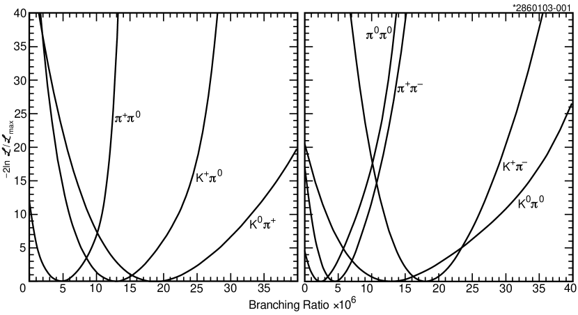
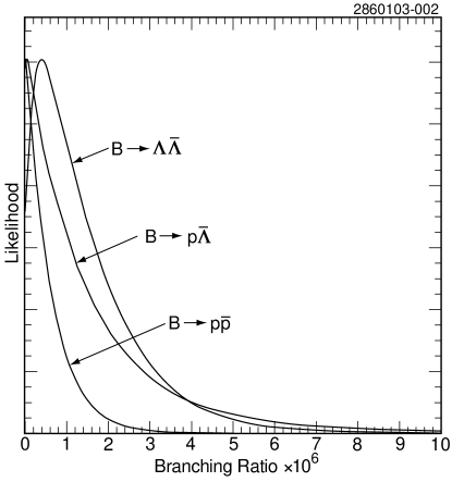
Particle identification in CLEO II was limited, and modes with potential for $K/\pi$ misidentification, such as $B\to\pi^{+}\pi^{-}$ and $B\to K^{+}\pi^{-}$, were analyzed in terms of two-dimensional likelihood functions, $\mbox{${\cal L}$}(N_{\pi^{+}\pi^{-}},N_{K^{+}\pi^{-}})$. The improved $K/\pi$ separation in CLEO III however permits us to treat these modes independently in the new data. To combine CLEO II and CLEO III likelihood functions, therefore, we first project the two-dimensional CLEO II functions on to one-dimensional versions, using $\mbox{${\cal L}$}(x)=\int\mbox{${\cal L}$}(x,y)dy$, and then express in terms of branching ratios, $\mbox{${\cal L}$}(\mbox{${\cal B}$})=\mbox{${\cal L}$}(N_{sig}/({\mbox{$N_{B\bar{B}}$}}\epsilon))$. Systematic errors are included following the same method as described for CLEO III above to obtain a total CLEO II likelihood function for each mode. A final combined CLEO II and CLEO III likelihood function is then formed from the joint likelihood, $\mbox{${\cal L}$}_{\rm final}(\mbox{${\cal B}$})=\mbox{${\cal L}$}_{\rm CLEOII}(\mbox{${\cal B}$})\mbox{${\cal L}$}_{\rm CLEOIII}(\mbox{${\cal B}$})$. For $\pi\pi$ and $K\pi$ modes with non-zero yields we plot the negative log-likelihood functions in Fig. 1. Likelihood functions for the di-baryonic modes are shown in Fig. 2. Table 6 summarizes the final results, with separate entries for CLEO II results (extracted from the references and reproduced here for the convenience of the reader), CLEO III results, and the combined CLEO II and CLEO III results.

Figure 1: $-2\ln({\cal L}/{\cal L}_{max})$ distributions for CLEO II and CLEO III combined, for $K\pi$ and $\pi\pi$ modes with non-zero yield.

Figure 2: Likelihood functions for $B\to\mbox{${p\bar{p}}$}$, $B\to\mbox{${p\bar{\Lambda}}$}$, and $B\to\mbox{${\Lambda\bar{\Lambda}}$}$.

Table 6: Experimental results for CLEO II, CLEO III, and both datasets combined. Significances include systematic errors. Note that the $p{\bar{p}}$ analysis in Ref. 4 was done in only a subset of the full CLEO II dataset, so the “combined” result is simply the CLEO III upper limit. Upper limits are 90% confidence level. CLEO II results are taken from Ref. 4, except for the $K^{0}$$\overline{K^{0}}$, ${p\bar{\Lambda}}$  and ${\Lambda\bar{\Lambda}}$ modes which were analyzed in this work with the full CLEO II dataset for the first time.

	CLEO II - Ref. 4		CLEO III		Combined
Mode	Significance	${\cal B}$${\times 10^{6}}$	Significance	${\cal B}$${\times 10^{6}}$	Significance	${\cal B}$${\times 10^{6}}$
$\pi^{+}\pi^{-}$	4.2	4.3${}^{+1.6+0.5}_{-1.4-0.5}$	2.6	4.8${}^{+2.5+0.8}_{-2.2-0.5}$	4.4	4.5${}^{+1.4+0.5}_{-1.2-0.4}$
$\pi^{+}\pi^{0}$	3.2	5.6${}^{+2.6+1.7}_{-2.3-1.7}$	2.1	3.4${}^{+2.8+0.8}_{-2.0-0.3}$	3.5	4.6${}^{+1.8+0.6}_{-1.6-0.7}$
$\pi^{0}\pi^{0}$	2.0	$(<5.7)$	1.8	$(<7.6)$	2.5	$(<4.4)$
$K^{+}\pi^{-}$	$12$	17.2${}^{+2.5+1.2}_{-2.4-1.2}$	$>7$	19.5${}^{+3.5+2.5}_{-3.7-1.6}$	$>7$	18.0${}^{+2.3+1.2}_{-2.1-0.9}$
$\mbox{$K^{0}$}\pi^{+}$	7.6	18.2${}^{+4.6+1.6}_{-4.0-1.6}$	4.6	20.5${}^{+7.1+3.0}_{-5.9-2.1}$	$>7$	18.8${}^{+3.7+2.1}_{-3.3-1.8}$
$K^{+}\pi^{0}$	$6.1$	11.6${}^{+3.0+1.4}_{-2.7-1.3}$	$5.0$	13.5${}^{+4.0+2.4}_{-3.5-1.5}$	$>7$	12.9${}^{+2.4+1.2}_{-2.2-1.1}$
$\mbox{$K^{0}$}\pi^{0}$	4.9	14.6${}^{+5.9+2.4}_{-5.1-3.3}$	3.8	11.0${}^{+6.1}_{-4.6}\pm 2.5$	5.0	12.8${}^{+4.0+1.7}_{-3.3-1.4}$
$K^{+}K^{-}$	-	$(<1.9)$	-	$(<3.0)$	-	$(<0.8)$
$\mbox{$K^{0}$}K^{-}$	-	$(<5.1)$	-	$(<5.0)$	-	$(<3.3)$
$K^{0}$$\overline{K^{0}}$	-	$(<6.1)$	-	$(<5.2)$	-	$(<3.3)$
${p\bar{p}}$	-	$(<7.0)$	-	$(<1.4)$	-	$(<1.4)$
${p\bar{\Lambda}}$	-	$(<2.0)$	-	$(<3.2)$	-	$(<1.5)$
${\Lambda\bar{\Lambda}}$	-	$(<1.8)$	-	$(<4.2)$	-	$(<1.2)$

IX Physically Interesting Ratios and the Phase of $V_{ub}$

As discussed in the introduction, it is possible to extract information about the phase of $V_{ub}$ from these charmless $B$ decay data. The method of Reference 3 is based on two ratios of the branching fractions which we have measured and reported above. Using the notation of this reference, and combining statistical and systematic errors in quadrature, the ratios are found to be:

$$R_{*}\equiv\frac{\mbox{${\cal B}$}(B^{\pm}\to K^{0}\pi^{\pm})}{2\mbox{${\cal B}$}(B^{\pm}\to K^{\pm}\pi^{0})}=0.73\pm 0.21,$$ (8)

and

$$\epsilon_{exp}\equiv\tan\theta_{C}\frac{f_{K}}{f_{\pi}}\left[\frac{2\mbox{${\cal B}$}(B^{\pm}\to\pi^{\pm}\pi^{0})}{\mbox{${\cal B}$}(B^{\pm}\to K^{0}\pi^{\pm})}\right]^{1/2}=0.18\pm 0.04.$$ (9)

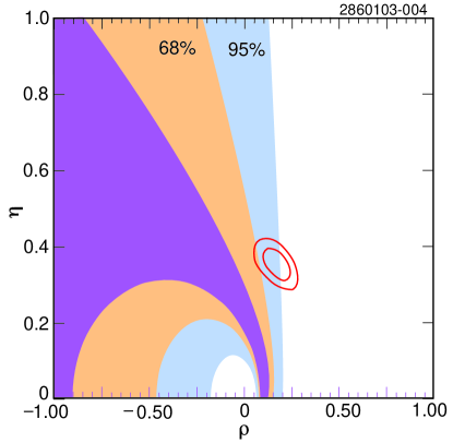
We see that the precision available with the CLEO data is about 20-30% in these quantities. With data from the BABAR and Belle experimentsbabarandbelle we can make world (weighted) averages of branching ratios and reach 10-15% experimental precision in the critical ratios: $R_{*}=0.71\pm 0.09$ and $\epsilon_{exp}=0.21\pm 0.02$. These numbers in turn indicate a preferred region for $\gamma=Arg(\mbox{$V_{ub}$})$ which is greater than 90^∘alan . Using these world-averaged data we construct contours in the $\rho-\eta$ plane according to prescription of Reference 3 and display the result in Figure 3. The dark band represents the experimental central value convolved with theoretical uncertainties; lighter bands show the additional coverage when 68% and 95% experimental confidence regions are included. For reference we also overlay 68% and 95% confidence level ellipses of the preferred apex of the unitarity triangle as obtained in a standard analysis based on $B$ mixing, $\sin 2\beta$, $V_{ub}$, and kaon decaysstochhi . An intriguing discrepancy between these regions is noticeable. In the short term the most substantial progress to be made will be in reducing the statistical errors on the branching ratios of charmless $B$ decay modes. If discrepancies survive there could be non-trivial implications for the Standard Model, as discussed in Ref. 3.

Figure 3: Confidence contours in the $\eta-\rho$ plane. The shaded bands represent regions allowed by the world-averaged charmless $B$ decay measurements while the ellipsoids represent 68% and 95% contours from conventional global fits to heavy quark measurements. The dark shaded region corresponds to the experimental central values of the charmless data, smeared by theoretical uncertainty. See text for details and references.

X The $\mbox{${\cal B}$}(B\to DK)/\mbox{${\cal B}$}(B\to D\pi)$ ratio

Figure 4: CLEO III data: the $M_{B}$ distribution for $B^{-}\rightarrow D^{0}\pi^{-}$ (left) and $B^{-}\rightarrow D^{0}K^{-}$ (right) candidates.

In view of the good $K/\pi$ separation in CLEO III data we also report a new determination of the ratio $\mbox{${\cal B}$}(B^{-}\to D^{0}K^{-})/\mbox{${\cal B}$}(B^{-}\to D^{0}\pi^{-})$ which benefits substantially from good particle identification. The original CLEO II publication is available in Ref. abi .

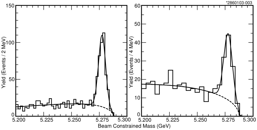
For this analysis, $D^{0}$ candidates are reconstructed in three secondary modes, $D^{0}\to K^{-}\pi^{+}$, $D^{0}\to K^{-}\pi^{+}\pi^{0}$, and $D^{0}\to K^{-}\pi^{+}\pi^{-}\pi^{+}$. Requirements for the $B\to D^{0}h^{-}$ modes include a 30 MeV $D^{0}$ mass cut, a 100 MeV $\Delta E$ cut, and standard particle ID as described previously on both the primary $h^{-}$ from the $B$ and on the secondary kaon from the $D^{0}$. The $\pi^{0}$ mass for the $D^{0}{\rightarrow}K^{-}\pi^{+}\pi^{0}$ mode is required to be within 30 MeV of its nominal mass. For the $D^{0}K$ likelihood fit, $D^{0}\pi$ is included as a cross-feed background, and corresponds to approximately 50% of the DK yield shown in Fig. 4. (Both $D^{*}\pi$ and $D\rho$ were found not to be significant backgrounds to either signal mode.) Fig. 4 shows $M_{B}$ distributions for $B^{-}\to D^{0}\pi^{-}$ and $B^{-}\to D^{0}K^{-}$ candidates with the likelihood fit shape superimposed.

Combining the three $D^{0}$ submodes, we find

$$\frac{\mbox{${\cal B}$}(B^{-}{\rightarrow}D^{0}K^{-})}{\mbox{${\cal B}$}(B^{-}{\rightarrow}D^{0}\pi^{-})}=(9.9^{+1.4+0.7}_{-1.2-0.6})\mbox{${\times 10^{-2}}$}.$$ (10)

Most systematic errors cancel in this ratio, with only a small residual arising from the particle identification requirements imposed on the primary $\pi/K$ in both numerator and denominator.

XI Summary

We have presented final results from the CLEO experiment on charmless hadronic $B$ decays. The decay modes include the ten $\pi\pi$, $K\pi$, and KK final states as well as the dibaryonic states $p\bar{p}$, $p\bar{\Lambda}$ and ${\Lambda\bar{\Lambda}}$. In addition we have presented a new determination of the ratio of branching ratios $\mbox{${\cal B}$}(B\to DK)/\mbox{${\cal B}$}(B\to D\pi)$. The results are based on the full CLEO II and CLEO III data samples totalling 15.3 ${\rm fb}^{-1}$ at the $\Upsilon(4S)$, and supercede previously published results by this collaboration.

XII Acknowledgements

We gratefully acknowledge the effort of the CESR staff in providing us with excellent luminosity and running conditions. M. Selen thanks the Research Corporation, and A.H. Mahmood thanks the Texas Advanced Research Program. This work was supported by the National Science Foundation, and the U.S. Department of Energy.

References

- (1) Y.-Y. Keum, H.-N. Li, and A.I. Sanda, arXiv:hep-ph/0201103; M. Neubert, JHEP 9902 (1999) 014; M. Neubert and J.L. Rosner, Phys. Rev. Lett. 81, 5076 (1998); M. Neubert and J.L. Rosner, Phys. Lett. B 441, 403 (1998); M. Neubert, Phys. Lett. B 424, 2752 (1998); R. Fleischer and T. Mannel, Phys. Rev. D 57, 2752 (1998)
- (2) M. Gronau and D. Wyler, Phys. Lett. B 265, 172 (1991)
- (3) M. Neubert, ArXiv:hep-ph/0207327, CLNS-02/1794; M. Beneke, G. Buchalla, M. Neubert, and C.T. Sachrajda, Nucl. Phys. B 606, 245 (2001); M. Beneke, G. Buchalla, M. Neubert, and C.T. Sachrajda, Phys. Rev. Lett. 83, 1914 (1999);
-
(4)
CLEO publications on charmless hadronic B decays:
(a) D. M. Asner et al., Phys. Rev. D 65, 031103 (2002) ; (b) R.A. Briere et al., Phys. Rev. Lett. 86, 3718 (2001); (c) D. Cronin-Hennessy et al.,Phys. Rev. Lett. 85, 515 (2000); (d) S.J. Richichi et al., Phys. Rev. Lett. 85, 520 (2000); (e) S. Chen et al., Phys. Rev. Lett. 85, 525 (2000); (f) C. Jessop et al., Phys. Rev. Lett. 85, 2881 (2000); (g) R. Godang et al., Phys. Rev. Lett. 1705, 26 (2000); (h) T.E. Coan et al., Phys. Rev. D 59, 111101 (1999); (i) B.H. Behrens et al., Phys. Rev. Lett. 80, 3710 (1998); (j) R. Godanget al., Phys. Rev. Lett. 80, 3456 (1998); (k) T. Bergfeld et al., Phys. Rev. Lett. 81, 272 (1998) ; (l) T.E. Browder et al., Phys. Rev. Lett. 81, 1786 (1998); (m) D.M. Asner et al., Phys. Rev. D 53, 1039 (1996); (n) M. Battle et al., Phys. Rev. Lett. 71, 3922 (1993); (p) C. Bebek et al., Phys. Rev. Lett. 62, 8 (1989) ; (q) D. Bortoletto et al., Phys. Rev. Lett. 62, 2436 (1989); (r) P. Avery et al., Phys. Lett. B 183, 429 (1987) - (5) B. Aubert, et al., BABAR Collaboration, ArXiv:hep-ex/0207055; B. Aubert, et al., BABAR Collaboration, ArXiv:hep-ex/0207063; B. Aubert, et al., BABAR Collaboration, ArXiv:hep-ex/0207065; B. Aubert, et al., BABAR Collaboration, ArXiv:hep-ex/0206053; B.C.K. Casey, et al., Belle Collaboration, Phys. Rev. D 66, 092002 (2002); K. Abe, et al., Belle Collaboration, Phys. Rev. D 66, 092002 (2002)
- (6) CLEO Collaboration, CLNS-94-1277; D. Peterson et al., Nucl. Instr. and Meth. A 478, 142 (2002)
- (7) Y. Kubota et al., (CLEO Collaboration), Nucl. Instr. and Meth. A 320, 66 (1992); T.S. Hill, Nucl. Instr. and Meth. A 418, 32 (1998).
- (8) M. Artuso et al., ”Construction, Pattern Recognition and Performance of the CLEO III LiF-TEA RICH Detector,” Presented at Fourth Workshop on RICH Detectors, Pylos Greece, June, 2002, to appear in the proceedings [hep-ex/0209009]
- (9) Particle Data Group, Phys. Rev. D 66, 010001 (2002).
- (10) J.P. Alexander et al., (CLEO Collaboration) Phys. Rev. Lett. 86, 2737 (2001)
- (11) R.A. Fisher, The Use of Multiple Measurements in Taxonomic Problems, Annals of Eugenics, 7, (1936) 179.
- (12) D. M. Asner et al., (CLEO Collaboration), Phys. Rev. D 53, 1039 (1996).
- (13) ARGUS Collaboration, H. Albrecht et al., Phys. Lett. B 241, 278 (1990); Phys. Lett. B 254, 288 (1991).
- (14) G. Fox and S. Wolfram, Phys. Rev. Lett. 241, 1581 (1978),
- (15) D. Cronin-Hennessy et al., (CLEO Collaboration), Phys. Rev. Lett. 285, 515 (2000) ;
- (16) Alan J. Magerkurth, Cornell University Ph.D thesis (unpublished) Measurement of Two Body B Meson Decays to Pions and Kaons with the CLEO III Detector.
- (17) A. Stocchi, Proceedings of the XXXIst Int’l Conf. on HEP, Amsterdam 2002. LAL 02-102; arXiv:hep-ph/0211245
- (18) M. Athanas et al., (CLEO Collaboration) Phys. Rev. Lett. 80, 5493 (1998)