Using Wavelets to reject background in Dark Matter experiments

Abstract

A method based on wavelet techniques has been developed and applied to background rejection in the data of the IGEX dark matter experiment. The method is presented and described in some detail to show how it efficiently rejects events coming from noise and microphonism through a mathematical inspection of their recorded pulse shape. The result of the application of the method to the last data of IGEX is presented.

PACs: 95.35+d: 14.80.Mz

Keywords: Dark Matter; Low background; Underground Detectors; Wavelets; Noise Rejection

I.G. Irastorza^a, A. Morales^a, S. Cebrián^a, E. García^a, J. Morales^a, A. Ortiz de Solórzano^a, S.B. Osetrov^b, J. Puimedón^a, M.L. Sarsa^a, J.A. Villar^a

1 Introduction

Experiments searching for rare event phenomena, like those looking for non-baryonic dark matter particles (axions or WIMPs), supposedly filling a substantial part of the galactic haloes, or those looking for the neutrinoless double beta decay have become of most relevance in Particle Physics and Cosmology. To find the nature of Dark Matter, the essential component of the Universe, which in its non-baryonic form might be (according to recent developments) responsible of $\sim$25-30 % of the dark energy/matter budget of a flat universe, is one of the big challenges of modern Cosmology. On the other hand, the old subject of nuclear double beta decay which has been the objective of many experimental efforts as an unique tool to explore the nature of the electron neutrino and to verify the lepton number conservation, has become recently of even greater importance after the confirmation that the neutrino has a non-zero mass. In fact, the existence of neutrinoless double beta decay may provide information on the absolute scale mass of the neutrino, its mass pattern and possibly on CP violation in the leptonic sector if the sensitivity of the experiments is able to reach the level of a few meV for the Majorana neutrino effective mass upper bound.

The signals to be expected in the two selected examples of rare event physics, have in common their low rates and so the main challenge to achieve the required sensitivity is to disentangle the signal from the various sources of background, which largely hide the expected signals. Consequently, the first basic requirement of these types of searches is to provide an ultra-low background environment, as well as to design specific techniques of shielding and background rejection.

In the particular case of dark matter searches, the expected signal is concentrated in the lowest part of the spectrum [1] often just above the threshold of the experiment. When the effective threshold of these experiments is fixed by the electronic baseline, random fluctuations of this baseline –electronic noise– can populate the energy range of interest with noise events. Actually this electronic noise becomes a primary source of background which is of special concern.

In this paper we describe a method which has been developed and successfully applied to the last data set of the IGEX dark matter experiment. In the section 2 we will describe briefly the IGEX experiment, just to understand the needs that led to the method presented in this paper. The details of the experiment can be found in ref. [2, 3] which contain also the scientific results of IGEX. In sections 3 and 4 the wavelet method itself and its calibration are described. We finish with the conclusions in section 5.

2 The Experiment

The IGEX experiment [2, 4], optimized for detecting ⁷⁶Ge double-beta decay, has been described in detail elsewhere. One of the IGEX detectors of 2.2 kg, enriched up to 86 % in ⁷⁶Ge, is being used to look for WIMPs interacting coherently with the germanium nuclei. Its active mass is $\sim 2.0$ kg, measured with a collimated source of ¹⁵²Eu. The full-width at half-maximum (FWHM) energy resolution is 2.37 keV at the 1333 keV line of ⁶⁰Co, and the low energy long-term energy resolution (FWHM) is less than 1 keV at the 46.5 line of the ²¹⁰Pb.

We refer to papers [3] and [5] where the latest results of the experiment (regarding dark matter searches) are presented and where the aspects related to the set-up of the experiment, shieldings, the data acquisition system, etc. are described. The threshold of the experiment is about 4 keV and the raw background registered in the region just above threshold is of a few tenths of counts per kg and day and per keV. The background and threshold achievements provide the best WIMP-nucleon cross-section versus WIMP mass ($\sigma$,m) exclusion plot for spin-independent interactions ever obtained by an experiment with no mechanism of nuclear/electron recoils discrimination for background rejection. As stressed in [3, 5], the background level at low energies is crucial to set the sensitivity of the experiment and this is illustrated by the fact that a moderate reduction of the low energy background would lead to a substantial improvement in the final exclusion. To deal with the worrysome noise component in this energy region trying its minimization, we developed the analysis method described in the present paper. The acquisition system for low energy data is implemented by splitting the preamplifier output pulses and routing them through two Canberra 2020 amplifiers having different shaping times. These amplifier outputs are converted using 200 MHz Wilkinson-type Canberra analog-to-digital converters (ADC), controled by a PC through parallel interfaces. The energy spectrum is built using the ADC output of one of the lines. In addition, the output pulse of one of the amplifiers is digitized and recorded for each event using a 800 MHz LeCroy 9362 digital scope. The digitized pulse encompasses a time window of 500 $\mu$s with a sampling resolution of 1 $\mu$s. This recorded pulse shape is analyzed off-line with the method described below and is formally referred as $f(t)$ in the following.

3 The method

Wavelets are mathematical tools that have been proven to be extremely useful in a number of different types of analysis [6]. In particular, they have been applied to the recognition and extraction of noise from certain sets of data. From a mathematical point of view, the so-called wavelet transforms can be viewed as extensions of the Fourier transforms, but with the addition of sensitivity to local features of the studied function. In fact, the set of functions which play the role of the $e^{i\omega t}$ in the Fourier transform are now $\psi_{a,b}(\frac{t-b}{a})$ derived from an original localized null-area wavelet function $\psi(t)$ by means of translations and contractions parameterized respectively by $b$ and $a$. Therefore, for a fixed wavelet function $\psi(t)$, the biparametric wavelet transform $[W_{\psi}f](a,b)$ of a given function $f(t)$ can be defined as:

$$[W_{\psi}f](a,b)=\frac{1}{\sqrt{a}}\int_{-\infty}^{\infty}f(t)\psi\left(\frac{t-b}{a}\right)dt$$ (1)

The above mentioned condition of null-area for $\psi(t)$, or admisibility condition, is derived from the requirement that no information loss must occur in the transformation (i.e. it must be invertible). Apart from this requirement, other properties are desirable in certain contexts, like continuity, gaussian shape, etc. Without entering into the mathematical details of the wavelet theory [6], and following a practical approach, the ”mexican hat” wavelet function $\psi(x)$ was chosen because it fitted most suitably our requirements:

$$\psi(x)\propto(1-x^{2})\exp\left(-\frac{1}{2}x^{2}\right)$$ (2)

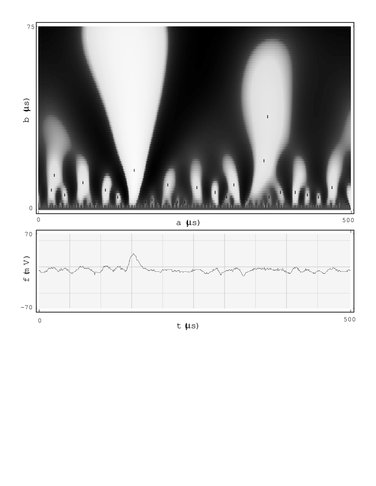
Figure 1: In the lower part a sample pulse corresponding to an event of about 4.5 keV is shown. In the upper part the 2-dimensional wavelet transform of the same pulse is presented. Lighter regions correspond to highest values of the transform function. The relative maxima are marked with dark spots. The highest maximum is clearly related with the presence of the true pulse, the others being caused by random fluctuations of the baseline.

As stated before, $f(t)$ is the pulse shape for each event as recorded by the data acquisition system. Following expression (1), the wavelet transform function $[W_{\psi}f](a,b)$ can be calculated numerically for each event. The resulting function is continuous due to the properties of the wavelet function used. So the relative maxima $(a_{i},b_{i})_{i}$ (where $i$ goes from 1 to $N$, being N the total number of maxima) can be calculated by means of an appropriate numerical algorithm. Let’s order the maxima $(a_{i},b_{i})$ according to the magnitude of the wavelet transform in that maxima, $\omega_{i}\equiv[W_{\psi}f](a_{i},b_{i})$, such that the first maximum $\omega_{1}$ is the highest one. In some sense, these maxima contain the information of the pulse. For instance, the position of the highest one in the $(a,b)$ plane is determined by the width and position in the time window of the event pulse itself, if present, and the others $(a_{i},b_{i})_{i=2...N}$ are the result of random fluctuations of the baseline along the time window encompassed by $f(t)$. That is illustrated in figure 1, where in the lower part a sample event pulse is shown (to give an idea of the vertical scale, the pulse correspond to an event of about 4.5 keV, i.e. just above our threshold). In the upper part of the figure the 2-dimensional wavelet transform of the same pulse is presented, lighter regions corresponding to higher values of the $[W_{\psi}f](a,b)$. The relative maxima are also marked with darker spots, the first one being clearly identified and corresponding to the true pulse, and the others corresponding to random fluctuations of the baseline.

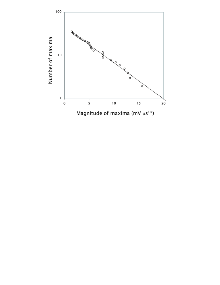
Figure 2: Distribution of the maxima $\omega_{i}$ ($i$ going from 2 to $N$) of the wavelet transform for a sample event and their fit to an exponential.

The key idea of the method is based on the comparison between the magnitude of the first maximum $\omega_{1}$ with the distribution of the others $\{\omega_{i}\}_{i=2...N}$. In fact, the mentioned distribution has been checked to be well modelled by a decaying exponential (this fact being related to the kind of wavelet function we are using). Figure 2 shows such a distribution for one event.

Now, the method consists of constructing the exponential distribution $D(w)=ke^{-\alpha w}$ which follows the baseline induced maxima in every event pulse shape and evaluate the parameter $P_{1}$ of the first maximum, defined as the normalized area of the distribution $D(w)$ which lies above the first maximum $w_{1}$:

$$P_{1}=\frac{\int_{w_{1}}^{\infty}D(w)dw}{\int_{0}^{\infty}D(w)dw}=e^{-\alpha w_{1}}$$ (3)

This parameter $P_{1}$ is the final outcome of the method for each event, and gives us, to a certain extent, an indication of the probability of the main pulse to have been generated randomly by the fluctuations of the baseline, being smaller for pulses farther from a noise-like pulse. Therefore, if $P_{1}$ is large enough, the event must be considered a noise fluctuation and should be rejected, otherwise, the event is kept. The reference value to decide if $P_{1}$ is large enough or not must be fixed by calibration of the method, and is explained in the following section.

4 Calibration

In order to fix the rejection criterion this method was applied to a calibration set of data. The calibration was performed with a ²²Na source which was introduced inside the shielding through a teflon probe producing a rate of events much higher than the standard background. The source provides an almost pure sample of ”true” events, i.e. events not coming from noise. The result of the method applied to this set of data is illustrated in figure 3 where the parameter $P_{1}$ (obtained as previously explained) versus energy is presented for each event of the calibration set. As expected, this parameter shows a clear correlation with the event energy. It is interesting to see that the same plot for the parameter $P_{2}$, defined similarly as $P_{1}$ but for the second maximum $w_{2}$, shown in figure 4 lacks completely this correlation, as this second maximum is related to some fluctuation of the baseline other than the true pulse. The same type of plot obtained for a background set of data is shown in figure 5. In this plot two different populations are clearly visible. One of them follows the same energy dependence than that of the calibration data and the other does not. This second type of events are identified as noisy fluctuations of the baseline that have triggered the acquisition system but no relevant pulse above threshold is present. From these plots a criterion of $P_{1}<0.01$ can be defined to distinguish the two populations of noise and data. Due to the limited statistics of the set of data available, it is hard to quantify the energy dependence of the loss of efficiency of the cut. However, from the presented plots one can state that it is negligible for events which lay a little above our threshold, whereas only in the very first keV above threshold it could be only a few percent.

Moreover, this method provides another way of rejection. The calculation of the first maximum of the wavelet transform provides the width of the corresponding pulse: $a_{1}$. This parameter is tightly constrained for true pulses due to the shaping. As can be seen in the figure 6, for our present set-up all of the low energy pulse widths are between 7 and 16 $\mu$s. This fact can be used to reject events with pulse widths outside this range. This argument allows to reject a small population of events which were not rejected by the previous method, fact that is illustrated in figure 7. They correspond to large lower-frequency fluctuations of the baseline presumably connected with microphonism. Due to the fact that they are not strictly random fluctuations in the sense previously considered, they could not be rejected before. The loss of efficiency of this cut is completely negligible.

5 Conclusions

We have presented a method based on wavelet techniques which is able to efficiently reject electronic noise and microphonism from the low energy –just above threshold– region. The method analyzes the recorded pulse shape of the event to extract information about the pulse height in comparison to the fluctuations of the baseline to set if the pulse can be assumed to be randomly generated by the fluctuations. This method was succesfully applied in the last data of the IGEX dark matter direct search. In figure 8 we show the low energy spectrum obtained with the last published 80 kg$\cdot$day of data of IGEX [5] showing the effective rejection achieved with the present method. About half of the background between 4 and 7 keV and about 20% between 7 and 10 keV was identified as noise and eventually rejected.

6 Acknowledgments

This work has been partially supported by MCYT, Spain, under contract No. FPA2001-2437. We are indebted to our IGEX colleagues for their collaboration in other tasks of the experiment. I.G.I. wish to thank Prof. J. Garay for his illuminating discussions on the wavelet transform.

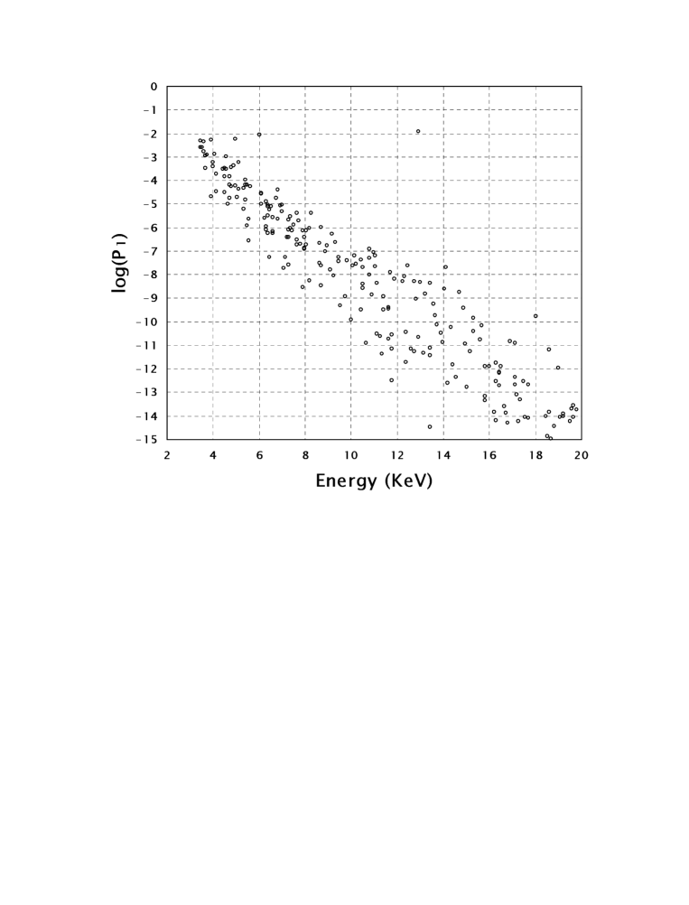
Figure 3: Scatter plot showing the parameter $P_{1}$ assigned to each event by the wavelet technique (described in the text) versus energy for a calibration set of data.

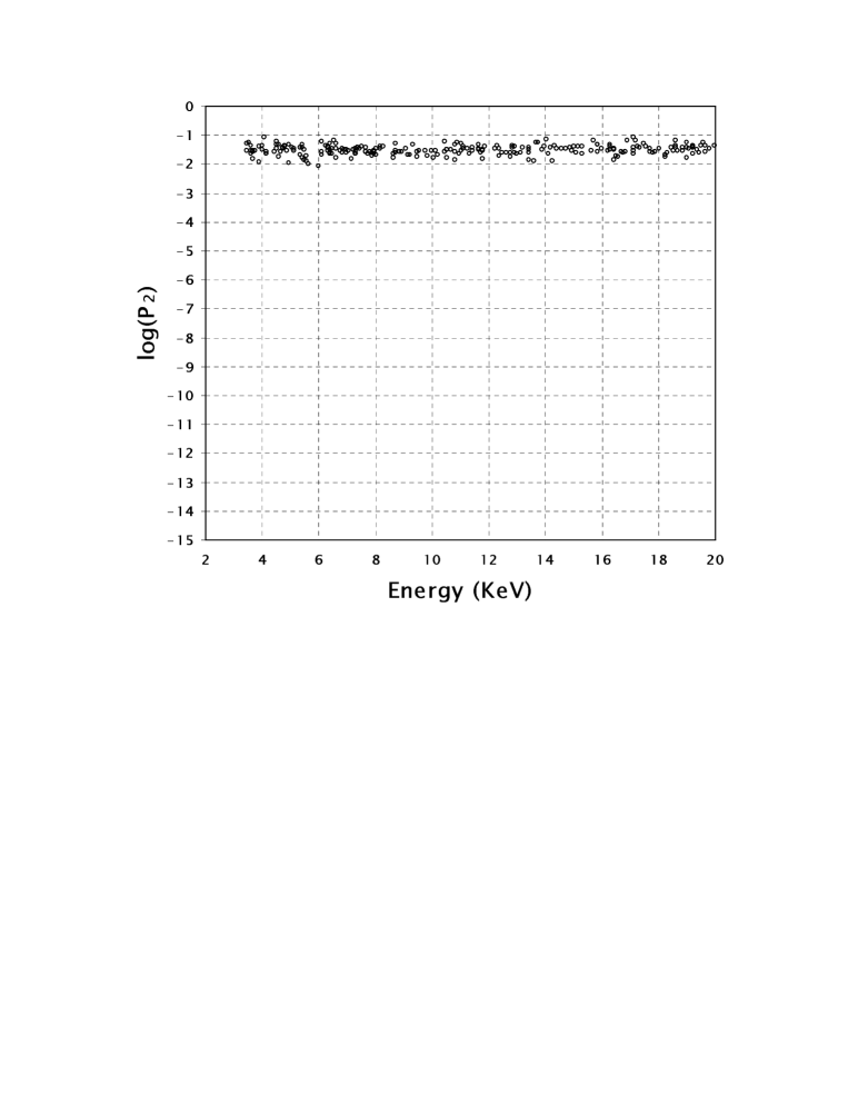
Figure 4: Scatter plot showing the parameter $P_{2}$ related to the second maximum of the wavelet transform versus the energy of the event (for a calibration set of data).

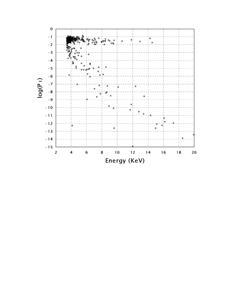
Figure 5: Same as figure 3 but for background data. The populations of noise and data are well separated above 4 keV.

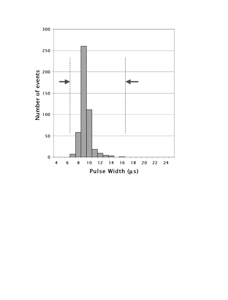
Figure 6: Distribution of pulse widths for a calibration set of data considering only events from 4 to 40 keV. All of them are in the range 7 to 16 $\mu$s.

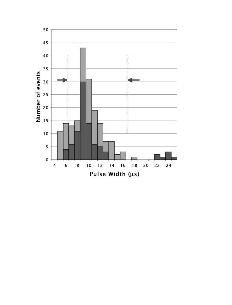
Figure 7: Distribution of pulse widths for a background set of data (considering only events from 4 to 40 keV), before and after the rejection based on the criterion on the parameter $P_{1}$. It can be appreciated some events with large width (above 16 $\mu$s) which are not rejected by such criterion.

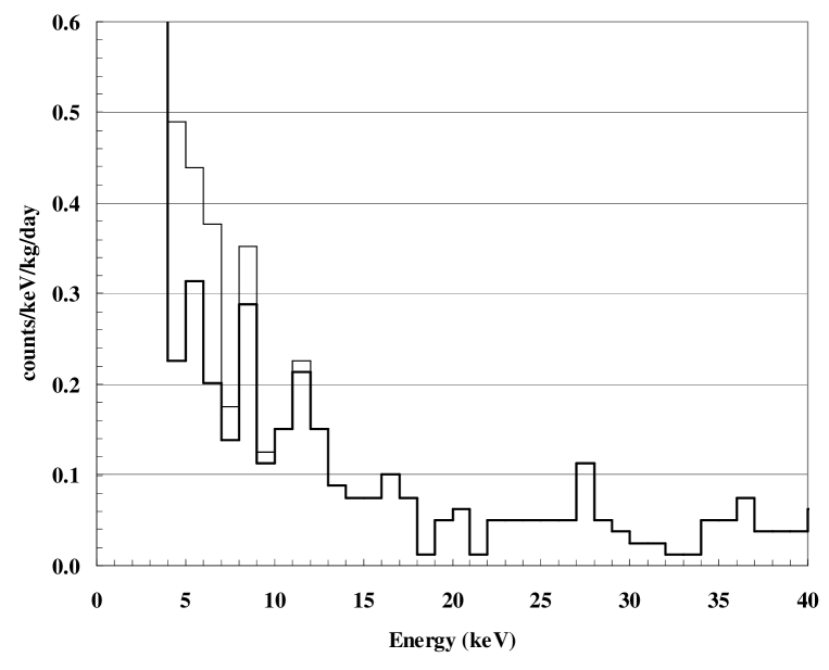
Figure 8: Low energy spectrum of the last published 80 kg$\cdot$day of data of IGEX before (thin line) and after (thick line) the application of the wavelet rejection method.

References

- [1] For a recent survey of WIMP experimental detection, see for instance A. Morales, Nucl. Phys. B (Proc. Suppl.) 87 (2000) 477, [astro-ph/9912554] and A. Morales, Nucl. Phys. B (Proc. Suppl.) 110 (2002) 39, [astro-ph/0112550]. N. J. C. Spooner, V. A. Kudryavtsev, Talk at the International Europhysics Conference on High Energy Physics, [astro-ph/0111053].
- [2] C. E. Aalseth, F.T. Avignone, R.L. Brodzinski, J.I. Collar, E. Garcia, D. Gonzalez, F. Hasenbalg, W.K. Hensley, I.V. Kirpichnikov, A.A. Klimenko, H.S. Miley, A. Morales, J. Morales, A. Ortiz de Solorzano, S.B. Osetrov, V.S. Pogosov, J. Puimedon, J.H. Reeves, A. Salinas, M.L. Sarsa, A.A. Smolnikov, A.S. Starostin, A.G. Tamanian, A.A. Vasenko, S.I. Vasilev, J.A. Villar [IGEX Collaboration], Phys. Rev. C 59 (1999) 2108.
- [3] A. Morales, C.E. Aalseth, F.T. Avignone, III, R.L. Brodzinski, S. Cebrian, E. Garcia, D. Gonzalez, W.K. Hensley, I.G. Irastorza, I.V. Kirpichnikov, A.A. Klimenko, H.S. Miley, J. Morales, A. Ortiz de Solorzano, S.B. Osetrov, V.S. Pogosov, J. Puimedon, J.H. Reeves, M.L. Sarsa, S. Scopel, A.A. Smolnikov, A.G. Tamanian, A.A. Vasenko, S.I. Vasilev, J.A. Villar [IGEX Collaboration], Phys. Lett. B 489 (2000) 268 [hep-ex/0002053].
- [4] D. Gonzalez, C.E. Aalseth, F.T. Avignone, R.L. Brodzinski, S. Cebrian, E. Garcia, W.K. Hensley, I.G. Irastorza, I.V. Kirpichnikov, A.A. Klimenko, H.S. Miley, A. Morales, J. Morales, A. Ortiz de Solorzano, S.B. Osetrov, V.S. Pogosov, J. Puimedon, J.H. Reeves, M.L. Sarsa, S. Scopel, A.A. Smolnikov, A.G. Tamanian, A.A. Vasenko, S.I. Vasilev, J.A. Villar [IGEX Collaboration], Nucl. Phys. Proc. Suppl. 87 (2000) 278.
- [5] A. Morales, C.E. Aalseth, F.T. Avignone, III, R.L. Brodzinski, S. Cebrian, E. Garcia, I.G. Irastorza, I.V. Kirpichnikov, A.A. Klimenko, H.S. Miley, J. Morales, A. Ortiz de Solorzano, S.B. Osetrov, V.S. Pogosov, J. Puimedon, J.H. Reeves, M.L. Sarsa, A.A. Smolnikov, A.G. Tamanyan, A.A. Vasenko, S.I. Vasilev, J.A. Villar [IGEX Collaboration], Phys. Lett. B 532 (2002) 8 [hep-ex/0110061].
- [6] See for instance S. Mallat, A wavelet tour of signal processing, Ac.Press, 1998 and C. Chui, Wavelets: a tutorial in Theory and Applications, Ac.Press, 1992.