Polarized Structure Functions in the Valence Quark and Resonance Regions and the GDH Sum.

Abstract

I present in this paper the neutron spin physics program in Hall A at Jefferson Laboratory using a polarized ³He target. The program encompasses several completed experiments, in which, valuable spin observables (spin dependent structure functions) were measured in order to learn about how the nucleon spin arises from the behavior of the constituents. These experiments also offer a ground for testing our understanding of the strong regime of quantum chromodynamics (QCD) the theory of strong interactions through the determination of moments of these structure functions.

1 INTRODUCTION

Technical advances for producing polarized beams and polarized targets in the early 80’s triggered a novel experimental effort at SLAC which provided for the first measurement of the proton spin asymmetry $A_{1}^{p}(x,Q^{2}$) [1]. The limited $x$ range of this measurement led to an interpretation of the results consistent with the predictions of a naive non-relativistic constituent quark model (CQM). However after EMC at CERN [2] extended the range of the SLAC measurement to significantly lower values of $x$, a different and surprising picture of the spin structure of the nucleon emerged. By combining the measured $\Gamma_{1}=\int_{0}^{1}g_{1}(x,Q^{2})dx$ with the neutron and hyperons $\beta$ decays within the CQM it was found that only a small fraction of the total nucleon spin was accounted for by quarks. Since then, enormous theoretical and experimental progress has been achieved in understanding the nucleon spin structure[3, 4]. The original findings of EMC were confirmed and measurements on the neutron allowed the test of the Bjorken sum rule [5] to $<10$% level. This accurate test was only possible after the sum rule, originally derived at $Q^{2}\rightarrow\infty$ using current algebra, was re-derived using the technique of operator product expansion (OPE) within QCD [6, 7, 8, 9]. This step was essential in order to calculate the corrections necessary to evolve this sum rule to $Q^{2}$ values accessible experimentally. In these studies most of the measurements on the nucleon spin structure functions were performed at large $Q^{2}$ above 1 GeV². Nevertheless to take full advantage of the OPE and test its applicability in the strong regime of QCD, it was understood that measurements of the nucleon spin structure below $Q^{2}$ = 1 GeV² and in the resonance region would be important for determining the size of the higher twists corrections. In this connection it was realized that the Bjorken sum rule was only a special case of a more general sum rule known as the ”extended” Gerasimov-Drell-Hearn (GDH) sum rule which coincides with the GDH sum rule at $Q^{2}=0$ and with the Bjorken sum rule at $Q^{2}\rightarrow\infty$.

Furthermore, higher moments of the spin structure functions are connected with specific twist matrix elements (observables) which can be evaluated using Lattice QCD [10, 11]. The advantage of measuring higher moments of the spin structure functions is twofold, 1) the kinematical region which gives most of the contribution to these moments is experimentally accessible 2) calculations of specific matrix elements related to these moments through OPE are possible using Lattice QCD.

I will present here results of two experiments performed at Jefferson Lab in Hall A that address two areas of the above mentionned concerning the spin structure of the neutron. First we present results of a precision measurement (E99-117) of the neutron asymmetry $A_{1}^{n}$ in the valence region where the existing world data could not confirm the expected behavior from either the CQM or pQCD due to a poor statistical precision. Second we present results of a measurement of both $g_{1}$ and $g_{2}$ (E94-010) through the resonance region at a $Q^{2}$ ranging from 1 GeV/c to 0.1 GeV/c and the neutron $\Gamma_{1}^{n}$ and $d_{2}^{n}$ are evaluated in the same range of $Q^{2}$ connecting the perturbative regime to the strong regime of QCD.

2 EXPERIMENTAL METHOD AND SETUP

The experiments described in this presentation share the same experimental setup [12]. They were carried out at Jefferson Lab in Hall A using a highly polarized electron beam (70-80%) with an average current up to 15$\mu A$ and a high pressure polarized (on average between 30% and 40% in-beam) ³He target with the highest polarized luminosity in the world. The target is based on the spin exchange principle where rubidium atoms are polarized by optical pumping and their polarization is transferred to the ³He atoms via spin exchange collisions [13]. The target was polarized either parallel or perpendicular to the direction of the electron beam and its polarization measured by three independent methods: NMR through the Adiabatic Fast Passage technique, Electron Paramagnetic Resonance technique (EPR) and elastic scattering off ³He. In each case the results of the three methods agreed within systematic errors.

The scattered electrons were detected using two HRS spectrometers which sat symmetrically on each side of the electron beam line to double the count rate. The spectrometers were equipped with standard detector packages which consists of two vertical drift chambers for momentum and scattering angle determination, a CO₂ gas Cherenkov counter and a double-layered lead-glass shower counter for particle identification [14]. The electron identification efficiency was 99% and the $\pi^{-}$ rejection factor was found to be better than 10⁴ for both spectrometers which was sufficient for all experiments. The momentum of each spectrometer was stepped through the relevant excitation spectrum at each incident energy of a given experiment. In many cases the comparison of the data between the two identical spectrometers at symmetric angles allowed us to minimize many of the systematic uncertainties.

3 SPIN AND FLAVOR DECOMPOSITION IN THE VALENCE QUARK REGION

Among the deep inelastic lepton scattering (DIS) spin observables important for understanding the structure of the nucleon at large $x$, the virtual photon-nucleon asymmetry $A_{1}^{n}$ and spin structure function $g_{1}^{n}$ are the most poorly known. This shortcoming is due to the small scattering cross sections in the large $x$ region combined with the lack of high polarized luminosity facilities. In the past experimental effort has gone into measuring $A_{1}^{n}$ and $g_{1}^{n}$ at low $x$, since it provides for most of the strength to $\Gamma_{1}$, resulting in a poor statistical precision in the world data for $x>0.4$. This region, however, is clean and unambiguous since it is not polluted by sea quarks and gluons and thus offers a unique opportunity to test predictions that are usually difficult if not impossible at low $x$. A very clean contribution of the ”valence quarks” can be expected when $x>0.5$. At present at large $x$ the world data are still consistent with the most naive of CQM’s which uses a static SU(6) symmetric wave function to describe the ground state of the nucleon. However, we know from the ratio of neutron to proton unpolarized structure functions measurements that this symmetry is broken in nature and thus the prediction is unrealistic.

The set of predictions of $A_{1}^{n}$ in the valence quark region falls into two categories, those of CQM’s which break SU(6) symmetry in the ground state wave function by hyperfine interaction [15, 16] which responsible for the N-$\Delta$ mass splitting, and those of perturbative QCD with a hadron helicity conservation (HHC) constraint [17, 18] as $x\rightarrow 1$ which break SU(6) symmetry dynamically. While both classes of models predict that $A_{1}^{n}\rightarrow 1$ when $x\rightarrow 1$ their $x$ dependence is noticeably different, allowing for a softer variation of $A_{1}^{n}$ towards unity in the case of the CQM’s. In the case where the HHC constraint is not imposed in pQCD calculations the results are rather a fit to the world data [20]. In this case the approach is to perform a pQCD analysis of the proton and neutron world data of the polarized structure functions at next-to-leading-order (NLO) and produce a global fit with a minimal number of parameters . This endeavor has been successful in the calculations by Bourelly, Soffer and Bucella  [21] using a statistical physical picture of the nucleon.

The difference between the approaches described above is more pronounced when the constituents flavor decomposition is performed. In the case where we consider a proton, we have $\Delta u(x)/u(x)\rightarrow 1$, $\Delta d(x)/d(x)\rightarrow 1$, for the case of pQCD with HHC models, and $\Delta u/u\rightarrow 1$, $\Delta d/d\rightarrow-2/3$ for the case of CQM’s. We notice that in the pQCD with HHC models $\Delta d/d$ changes sign from negative at low $x$ to positive at large $x$. This behavior is clearly different in the CQM model based on single flavor dominance where $\Delta d/d$ is negative at all $x$ values.

Furthermore, we mention exceptions to the models discussed above. A bosonized chiral quark model where the nucleon appears as a soliton in the meson fields was used to calculate $A_{1}^{n}$ in [22]. In [23] local quark-hadron duality is used to link the structure functions $g_{1}$ and $F_{1}$ at large $x$ with the $Q^{2}$ dependence of the nucleon electromagnetic form factors. A prediction was possible however we do not know how low in $x$ will this prediction works. Finally structure functions have been calculated in the bag model and the effect of the pion cloud on these functions was evaluated in [24].

At Jefferson Lab we are in a unique position to take advantage of the unprecedented polarized luminosity. The experiment was carried the highest available incident energy of 5.7 GeV. Both the $A_{\parallel}$ and $A_{\perp}$ asymmetries for ³He were extracted after correcting the raw asymmetries by the beam and target polarizations and the dilution factor at three kinematics: $x$ = 0.331, 0.474 and 0.61, and $Q^{2}$ = 2.738, 3.567 and 4.887 GeV², with $W^{2}$ = 6.426, 4.846 and 4.023 GeV² respectively. False asymmetries were checked by measuring asymmetries of the polarized beam scattering off an unpolarized ¹²C target and found to be negligible. Radiative corrections were applied to obtain the Born asymmetries and then, the asymmetry $A_{1}$ and the ratio of polarized to unpolarized structure functions $g_{1}/F_{1}$ of ³He were extracted using

$$A_{1}=\frac{A_{\parallel}}{D(1+\eta\xi)}-\frac{\eta A_{\perp}}{d(1+\eta\xi)}~{}~{}{\rm and}~{}~{}\frac{g_{1}}{F_{1}}=\frac{1}{D^{\prime}}\biggl{[}A_{\parallel}+\tan{(\theta/2)}A_{\perp}\biggr{]},$$ (1)

where $D$, $d$, $\eta$ and $\xi$ and $D^{\prime}$ are kinematical variables. Finally a ³He model which includes the $S$, $S^{\prime}$ and $D$ states and pre-existing $\Delta$ components in the ³He ground state wave function was used to extract $A_{1}^{n}$ and $g_{1}/F_{1}$of the neutron from that of ³He [26].

Figure 1: Left panel: Preliminary results of Jefferson Lab experiment E99-117 (solid squares) along with the world data (open symbols). The curves are predictions described in the text. Right panel: Spin and flavor dependent quark distributions extracted from the same experiment using equation (2). Hermes data error bars are statistical only. Error band shows the uncertainty due to neglecting $s$ and $\bar{s}$.

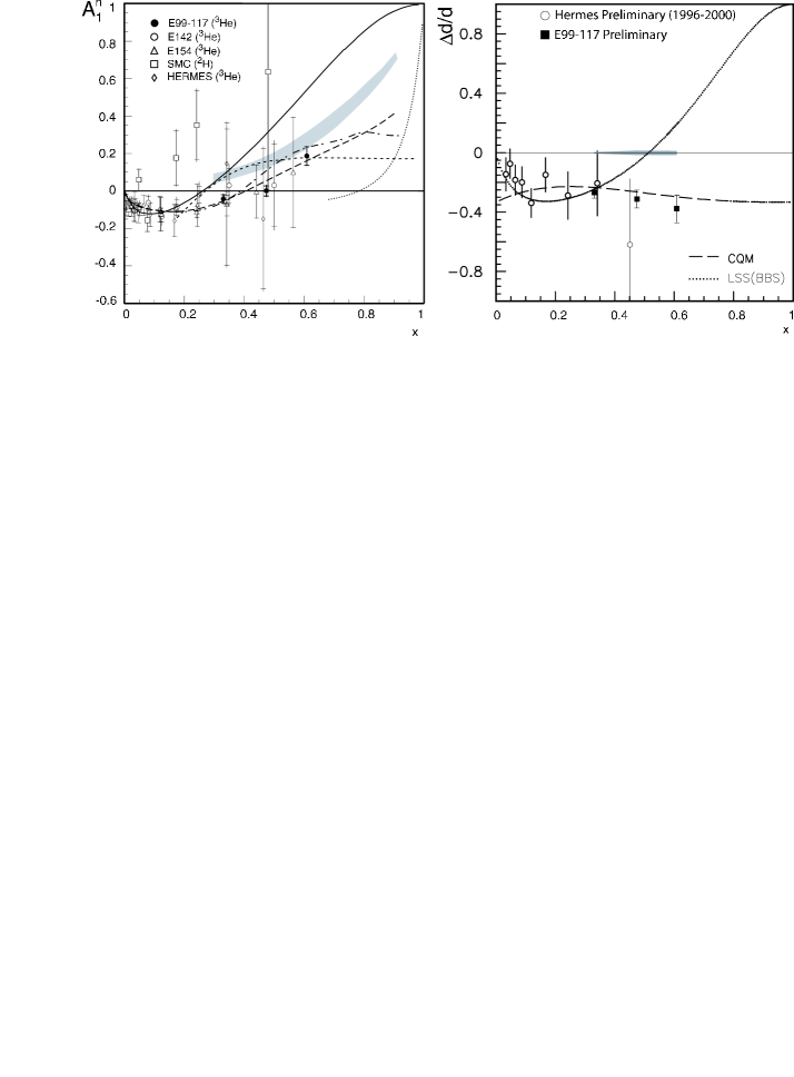
In Figure 1 (right panel) we show preliminary results of $A_{1}^{n}$. The first data point at $x=0.33$ is in good agreement with previous measurements. The data points show a clear change of sign of $A_{1}^{n}$ as $x$ increases and are compared with theoretical predictions. The total error in each point is dominated by the statistical error. The solid line is a pQCD HHC based on LSS(BBS) parameterization of ${g_{1}^{n}}/{F_{1}^{n}}$ [19], the long-dashed line is a prediction of ${g_{1}^{n}}/{F_{1}^{n}}$ from LSS 2001 parametrization at Q² = 5 GeV² without HHC constraints [20]. The shaded area is a range of predictions of $A_{1}^{n}$ from the constituent quark model [16] while the dot-dashed line is a calculation of the statistical model at Q² = 4 GeV² by Bourrely et. al. [21], and the dotted line is the local duality prediction by Melnitchouk [23]. Finally, the short dashed line is the chiral soliton model prediction at Q² = 3 GeV² by Weigel, Gamberg and Reinhardt [22]. Data from Hermes and SLAC are original values without being re-analyzed for the $\Delta$ contribution of the nuclear corrections.

Assuming that the strange quark distributions are negligible in the region $0.3<x<1$ we used the quark parton model interpretation of $g_{1}$ and $F_{1}$ to perform a flavor decomposition of the spin dependent quark distributions.

$$\frac{\Delta u}{u}=\frac{4}{15}\frac{g_{1}^{p}}{F_{1}^{p}}\biggl{(}4+\frac{d}{u}\biggr{)}-\frac{1}{15}\frac{g_{1}^{n}}{F_{1}^{n}}\biggl{(}1+4\frac{d}{u}\biggr{)},~{}~{}~{}~{}\frac{\Delta d}{d}=\frac{4}{15}\frac{g_{1}^{n}}{F_{1}^{n}}\biggl{(}4+\frac{u}{d}\biggr{)}-\frac{1}{15}\frac{g_{1}^{p}}{F_{1}^{p}}\biggl{(}1+4\frac{u}{d}\biggr{)}.$$ (2)

Here $u$ and $d$ represent the sum of quark and antiquark distributions. Using equation (2) and the $d/u$ ratio extracted from the proton and deuteron structure functions data [25] we present in Fig. 1 (left panel) results of the down quark distributions obtained in E99-117 (filled squares) along with preliminary results of the HERMES semi-inclusive measurements (open circles) [27]. The solid line is a pQCD fit to the world data using the HHC constraint as $x\rightarrow 1$. The dashed line correspond to a non relativistic constituent quark prediction. It is clear that up to $x=0.6$ the data favor the CQM and is in violation with the HHC pQCD based calculations. We point out that this is consistent with the interpretation the recent $Q^{2}$ dependence of the proton electromagnetic form factors ratio measured at Jefferson Lab [28].

4 EXTENDED GDH SUM RULE AND TWIST-THREE MATRIX ELEMENT

In its extended form the GDH sum rule spans all range of momentum transfers and reads [30]:

$$4\int_{Q^{2}/2M}^{\infty}{g_{1}(\nu,Q^{2})\over M\nu^{2}}d\nu=S_{1}(Q^{2}),$$ (3)

where $g_{1}(\nu,Q^{2})$ is the spin structure function of the nucleon, $S_{1}$ the virtual Compton scattering amplitude, $\nu$ the energy transfer and $M$ the nucleon mass. Starting the integration in equation (3) from the pion production threshold this sum rule can be expanded around $Q^{2}=0$ using for example the heavy baryon chiral perturbation theory (HB$\chi$PT) [31].

$$\Gamma_{1}^{n}(Q^{2}) = -{Q^{2}\over 8M^{2}}\kappa_{n}^{2}+\frac{5.54}{2M^{2}}Q^{4}+\alpha\biggl{(}{Q^{2}\over M^{2}}\biggl{)}^{3}+...$$ (4)

where $\kappa_{n}$ is the anomalous magnetic moment of the neutron. The slope of the first term in the right hand side of equation (4) corresponds to the standard GDH sum rule [37] while the second term on the right hand side has been evaluated using HB$\chi$PT. Other evaluations are available [35, 36] and will be compared to the data below. In the large $Q^{2}$ region Eq. (3) takes another form. If we consider three quarks flavors and three-loop result for the twist-two component $\Gamma_{1}^{n}(Q^{2})$is given by [32]:

$$\Gamma_{1}^{n}(Q^{2}) = \sum_{i=2,4...}{{\mu_{i}}(Q^{2})\over(Q^{2})^{i-2\over 2}}=\mu_{2}^{n}(Q^{2})+\frac{\mu_{4}^{n}(Q^{2})}{Q^{2}}+...$$ (5)

$$= \Big{[}1-({\alpha_{s}\over\pi})-3.5833({\alpha_{s}\over\pi})^{2}-20.2153({\alpha_{s}\over\pi})^{3}\Big{]}\biggl{(}-{1\over 12}g_{A}+{1\over 36}a_{8}\biggr{)}$$

$$+ \Big{[}1-0.3333({\alpha_{s}\over\pi})-0.54959({\alpha_{s}\over\pi})^{2}-4.44725({\alpha_{s}\over\pi})^{3}\Big{]}~{}{1\over 9}\Sigma_{\infty}+...$$

where $g_{a}=1.257$ and $a_{8}=0.579$ [33] are the triplet and octet axial charge, respectively. $\Sigma_{\infty}$ is defined as the renormalization group invariant nucleon matrix element of the singlet axial current [34]. At large enough $Q^{2}$ the $\mu_{4}$ contribution becomes negligible.

Presently, there is a large set of data on the spin structure function at $Q^{2}\geq$ 1 GeV² used to determine $\Sigma_{\infty}$ and $\alpha_{s}$. However, below $Q^{2}=1$ GeV² the experimental situation is less than ideal, prompting for the investigation of higher twists as $Q^{2}$ decreases below 1 GeV². This experimental situation has now changed with the completion of experiment E94-010 which covers a Q² ranging from 0.1 GeV² to 1 GeV². In this experiment we have measured the helicity dependent electron scattering cross sections for excitations energies covering from the quasielastic region up to the deep inelastic region, thus including the resonance region. The longitudinal ($\Delta\sigma_{\|}$) and transverse ($\Delta\sigma_{\bot}$) cross section differences are formed from combining data taken with opposite beam helicity,

$$\Delta\sigma_{\|}={\sigma^{\downarrow\Uparrow}-\sigma^{\uparrow\Uparrow}},~{}~{}~{}~{}~{}~{}\Delta\sigma_{\bot}={\sigma^{\downarrow\Rightarrow}-\sigma^{\uparrow\Rightarrow}},$$ (6)

where ${\sigma^{\downarrow\Uparrow(\uparrow\Uparrow)}}$ and ${\sigma^{\downarrow\Rightarrow(\uparrow\Rightarrow)}}$ are spin dependent inclusive differential cross sections with the electron spin helicity anti-parallel (parallel) and anti-perpendicular (perpendicular) to the target spin direction. The ³He spin structure functions $g_{1}(x,Q^{2})$ and $g_{2}(x,Q^{2})$ were extracted from the expression:

$$g_{1}(x,Q^{2}) = {MQ^{2}\nu\over 4\alpha_{e}^{2}}{E\over E^{\prime}}{1\over E+E^{\prime}}\biggl{[}\Delta\sigma_{\|}+\tan(\theta/2)\Delta\sigma_{\bot}\biggr{]}$$ (7)

$$g_{2}(x,Q^{2}) = {MQ^{2}\nu^{2}\over 4\alpha_{e}^{2}}{1\over 2E^{\prime}(E+E^{\prime})}\biggl{[}-\Delta\sigma_{\|}+\frac{E+E^{\prime}\cos{\theta}}{E^{\prime}\sin{\theta}}\Delta\sigma_{\bot}\biggr{]}$$ (8)

where $E$ and $E^{\prime}$ the incident and the scattered electron energy respectively, $\theta$ is the scattering angle, $M$ is the nucleon mass and $\alpha_{e}$ is the electromagnetic fine coupling constant.

Figure 2: Left panel: Preliminary results of the $Q^{2}$ evolution of $\Gamma_{1}^{n}$ from JLab experiment E94-010 along with the world data from DIS and theoretical calculations (see text). Right panel: Preliminary results of the twist three matrix element $d_{2}^{n}$ compared to SLAC E155X results and theoretical predictions. (see text).

The integral $\Gamma_{1}(Q^{2})$ for the neutron is evaluated by first performing the integration of the ³He response at constant $Q^{2}$ from the nucleon single pion production threshold to the lowest $x$ measured in the experiment. We then subtracted a small contribution due to the quasielastic tail and applied nuclear corrections to the integral following the procedure described in ref. [38]. We estimated the missing deep inelastic contribution in the range 2 GeV $<W<$ 30 GeV according to the parametrization of Thomas and Bianchi parametrization [39].

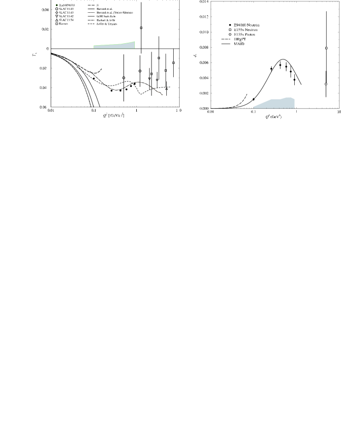
In Fig. 2 (left panel), we show $\Gamma_{1}^{n}(Q^{2})$ at five values of $Q^{2}$ from 0.1 to about 1 GeV² by step of 0.2 GeV² (solid circles) compared to the world data (open symbols). The band located around zero represents the size of systematic errors. At low $Q^{2}$ the lines correspond to $\chi$PT calculations by Bernard et. al. [35] (short dashed-dot line) without vector mesons and by Bernard et. al. [36] (dotted line) with vector mesons, respectively. The long dashed line is a calculation by Ji et. al. [30, 31] using heavy baryon $\chi$PT. The solid black line represents the GDH result. The comparison with our data shows that beyond $Q^{2}$=0.1 GeV² these calculations do not reproduce the trend of the data because the $\Delta$ degrees of freedom might become important but are not included in both $\chi$PT calculations. At moderate and large $Q^{2}$ two calculations, one by Soffer and Terayev [42] (short dashed curve), the other by Burkert and Ioffe [43] (long dash-dot line) are plotted. Soffer and Terayev assume that the integral over $g_{T}=g_{1}+g_{2}$ varies smoothly from high $Q^{2}$ where $g_{2}\approx 0$ down to $Q^{2}=0$. Using their prediction for this integral and subtracting the contribution from $g_{2}$ using the Burkhardt Cottingham sum rule [44] gives the short dashed curve in Fig. 2, which agree relatively well with the data. Burkert and Ioffe consider the contributions from the resonances using the code AO, and the nonresonant contributions using a simple higher-twist type form fitted to the deep-inelastic data. Their model is constrained to fit both the GDH and the deep-inelastic limits, and it describes the data quite well.

In the high $Q^{2}$ regime, using OPE, the $d_{2}$ matrix element defined as

$$d_{2}(Q^{2})=\int_{0}^{1}x^{2}[2g_{1}(x,Q^{2})+3g_{2}(x,Q^{2})]dx,$$ (9)

is shown to be a measure of the electric and magnetic polarizabilities of the color field [4]. At small $Q^{2}$, a region covered by our data, its conventional interpretation in terms of higher twist is not obvious. A recent publication [41] gives a new insight in this regard at low $Q^{2}$ using rather $\chi$PT. Thus, the $Q^{2}$ evolution of $d_{2}$ is also a quantity that can shed some light on the strong interaction in the nucleon.

In Fig. 2 (right panel), the $d_{2}$ matrix element is shown at several values of $Q^{2}$ where the integration in equation (9) excludes the elastic peak. The results of this experiment are the solid circles and the grey band represents their corresponding systematic uncertainty. The SLAC E155 [46] proton (open circle) and neutron (open square) results are also shown. The solid line is the MAID calculation[40] while the dashed line is a Heavy Baryon $\chi$PT calculation[41] valid only a very low $Q^{2}$. The Lattice prediction [11] at $Q^{2}$ = 5 GeV² for the neutron $d_{2}$ matrix element ( not shown here ) is negative but close to zero. We note that all models predict $d_{2}^{n}$ to be negative or zero at large $Q^{2}$. At moderate $Q^{2}$ the data of E94-010 show a positive $d_{2}^{n}$ but decreasing perhaps to zero at high $Q^{2}$. The SLAC data also show a positive $d_{2}^{n}$ value but with a rather large error bar. More measurements are needed to have a complete determination of the transition from low to very high $Q^{2}$ of this important matrix element.

5 CONCLUSION

In summary, we presented results of two experiments at Jefferson Lab Hall A which took advantage of the highly polarized beam and high pressure polarized ³He target to investigate the internal spin structure of the neutron in the perturbative and the strong regimes of QCD. In E99-117 we have determined the world most precise spin and flavor dependent distribution in the valence region. The results are more in line with the constituent quark model than with the HHC constrained pQCD prediction. In experiment E94-010 we have measured both $g_{1}$ and $g_{2}$ in the resonance region allowing for the first time to study the neutron integrals $\Gamma_{1}^{n}$ and the twist three matrix element $d_{2}^{n}$ from the pQCD regime to a regime where chiral perturbation theory might give us more insight into the structure of the nucleon. With time we expect Lattice QCD to make predictions in the intermediate region.

6 ACKNOWLEDGMENTS

The work presented here was supported in part with funds provided to the Nuclear and Particle Group at Temple University by the U.S. Department of Energy (DOE) under contract number DE-FG02-94ER40844. The Southeastern Universities Research Association operates the Thomas Jefferson National Accelerator Facility for the DOE under contract DE-AC05-84ER40150

References

- [1] V. H. Hughes and J. Kuti, Ann. Rev. Nucl. Sci 33, 611 (1983).
- [2] EMC, J. Ashman et. al., Phys. Lett. B206, 364 (1988); Nucl. Phys. B328, 1 (1989).
- [3] E. W. Hughes and R. Voss, Ann. Rev. Nucl. Part. Sci. 49,303 (1999).
- [4] B. W. Filippone and X. Ji, Adv. in Nucl. Phys. 26, 1 (2001).
- [5] J.D. Bjorken, Phys. Rev. 148, 1467 (1966); Phys. Rev. D1, 1376 (1970).
- [6] J. Kodaira, S. Matsuda, K Sasaki and T. Uematsu, Nucl. Phys. B159, 99 (1979).
- [7] J. Kodaira, Nucl. Phys. B165, 129 (1980).
- [8] S. A. Larin and J. A. M. Vermaseren, Phys. Lett. B259, 345 (1991).
- [9] E.V. Shuryak and A.I. Vainshtein, Nucl. Phys. 201, 141 (1982).
- [10] M. Fukugita, et al., Phys. Rev. Lett. 75, 2092 (1995).
- [11] M. Gockeler, et al., Phys. Rev. D63, 074506 (2001).
- [12] Details of experiments at www.jlab.org/e99117/ and www.jlab.org/e94010/.
- [13] T.G. Walker and W. Happer, Rev. Mod. Phys. 69, 629 (1997).
- [14] B.D. Anderson et al., http://www.jlab.org/equipment/NIM.ps .
- [15] F. Close and T.W. Thomas, Phys. Lett. B212, 227 (1988).
- [16] N. Isgur, Phys. Rev. D59, 034013 (1999).
- [17] G.R. Farrar, R.D. Jackson, Phys. Rev. Lett. 35, 1416 (1975).
- [18] S.J. Brodsky, M. Burkhardt, I. Schmidt, Nucl. Phys. B441, 197 (1995).
- [19] E. Leader, A.V. Sidorov and D.B. Stamenov, Int. J. Mod. Phys. A13, 5573 (1998).
- [20] E. Leader, A.V. Sidorov and D.B. Stamenov, Eur. Phys. J. C23, 479 (2002).
- [21] C. Bourrely, J. Soffer and F. Bucella, Eur. Phys. J. C23, 479 (2002).
- [22] H. Weigel, L. Gamberg and H. Reinhardt, Phys. Lett. B399, 287 (1997); Phys. Rev. D55, 6910 (1997); H. Weigel and L. Gamberg, Nuc. Phys. A680, 48 (2000).
- [23] W. Melnitchouk, Phys. Rev. Lett. 86, 35 (2001).
- [24] A.W. Schreiber, A.I. Signal and A.W. Thomas, Phys.Rev. D44, 2653 (1991). A.W. Schreiber, P.J. Mulders, A.I. Signal and A.W. Thomas, Phys.Rev. D44, 2653 (1991).
- [25] W. Melnitchouk, A. W. Thomas, Phys. Lett. B377, 11 (1996).
- [26] F. Bissey et al., Phys. Rev. C65, 064317 (2002).
- [27] J. Wendland, http://hermes.desy.de/notes/pub/TRANS/Deltaq.5p.ps.gz.
- [28] C.W. De Jager, contribution to these proceedings.
- [29] M. Amarian et al., Phys. Rev. Lett. 89, 242301 (2002).
- [30] X. Ji, C. Kao and and J. Osborne, Phys. Lett. B472, 1 (2000).
- [31] X. Ji and J. Osborne, J. Phys. G27, 127 (2001).
- [32] X. Ji and W. Melnitchouk, Phys. Rev. D56, 1 (1997).
- [33] F.E. Close and R.G. Roberts, Phys. Lett. B336, 257 (1994).
- [34] S.A. Larin, Phys. Lett. B334 192 (1994).
- [35] V. Bernard, N. Kaiser and Ulf-G. Meissner, Int. J. Mod. Phys. E4, 1 (2000).
- [36] V. Bernard, T. Hemmert and Ulf-G. Meissner, Phys. Lett. B545, 105 (2002).
- [37] S.B. Gerasimov, Sov. J. Nucl. Phys. 2, 598 (1965); S.D. Drell and A.C. Hearn, Phys. Rev. Lett. 16, 908 (1966).
- [38] C.C. Degli Atti and S. Scopetta, Phys. Lett. B404, 223 (1997).
- [39] E. Thomas and N. Bianchi, Nucl. Phys. B82, 256 (2000).
- [40] D. Drechsel, S. Kamalov and L. Tiator, Phys. Rev. D63, 114010 (2001).
- [41] C. W. Kao, T. Spitzenberg and M. Vanderhaeghen, hep-ph/0209241 (2002).
- [42] J. Soffer and O. V. Teryaev, Phys. Lett. B545, 323 (2002).
- [43] V. D. Burkert and B. L. Ioffe, Phys. Lett. B296, 223 (1992).
- [44] H. Burkhardt and W. N. Cottingham, Ann. Phys. 56, 453 (1970).
- [45] Z.P. Li and Zh. Li, Phys. Rev. D50, 3119 (1994).
- [46] E155, P.L. Anthony et. al., hep-ph/0204028 (2002).