Proper-time Resolution Function for Measurement of Time Evolution of $B$ Mesons at the KEK B-Factory

Abstract

The proper-time resolution function for the measurement of the time evolution of $B$ mesons with the Belle detector at KEKB is studied in detail. The obtained resolution function is applied to the measurement of $B$ meson lifetimes, the $B^{0}\overline{B}{}^{0}$ oscillation frequency and time-dependent CP asymmetries.

, , , , , , , and , , and

1 Introduction

KEKB is an asymmetric electron-positron collider designed to produce boosted $B$ mesons [1]. At KEKB, electrons (8.0 GeV) and positrons (3.5 GeV) collide at a small $(\pm 11~{}{\rm mrad})$ crossing angle. Their annihilations produce $\Upsilon(4S)$ mesons moving nearly along the $z$ axis, defined as anti-parallel to the positron beam direction, with a Lorentz boost factor of $(\beta\gamma)_{\Upsilon}=0.425$, and decaying to $B^{0}\overline{B}{}^{0}$ or $B^{+}B^{-}$. Precise determination of the proper-time interval $(\Delta t)$ between the two $B$ meson decays is essential for the measurement of $B$ meson lifetimes, the ${B^{0}}{\overline{B}{}^{0}}$ oscillation frequency, and time-dependent CP asymmetries. Since the $B$ mesons are nearly at rest in the $\Upsilon(4S)$ center of mass system (cms), $\Delta t$ can be determined from the separation in $z$ between the two $B$ decay vertices ($\Delta z$). The average $\Delta z$ at KEKB is $c\tau_{B}(\beta\gamma)_{\Upsilon}\sim 200~{}\mu$m, where $\tau_{B}$ is the $B$ meson lifetime. In this article, we consider the analysis in which one of the $B$ decay vertices is determined from a fully reconstructed $B$ meson, while the other is determined using the rest of the tracks in the event.

In order to extract the true $\Delta t$ distribution from the observed $\Delta z$ distribution it is necessary to unfold the vertex detector resolution and (possible) bias in the measurement of $\Delta z$. Because the detector resolution is of the same order as the average $\Delta z$ at KEKB, an understanding of the resolution is crucial for precise measurements. For measurement of time-dependent quantities, we employ an unbinned maximum likelihood method. A probability density function for the likelihood fit is obtained as a convolution of a theoretical $\Delta t$ distribution with the resolution function.

This paper describes the resolution function developed for the precise measurement of $B$ meson lifetimes with fully-reconstructed hadronic decay final states at the Belle experiment [2]. The obtained resolution function is also applied to the measurements of the ${B^{0}}{\overline{B}{}^{0}}$ oscillation frequency [3] and time-dependent CP asymmetries [4].

The organization of the paper is as follows: We give a brief description of the Belle detector in Section 2. In Section 3, the method of vertex reconstruction is described. Details of the resolution function and its application to the data are described in Sections 4 and 5, respectively, followed by a conclusion in Section 6.

2 The detector

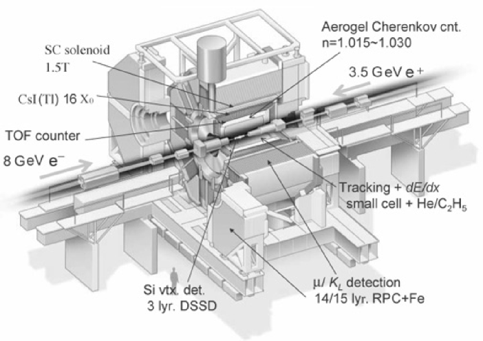
The Belle detector, shown schematically in Fig. 1, is a large-solid-angle magnetic spectrometer that consists of a three-layer silicon vertex detector (SVD), a 50-layer central drift chamber, a mosaic of aerogel threshold Cherenkov counters, time-of-flight scintillation counters, and an array of CsI(Tl) crystals located inside a superconducting solenoid that provides a 1.5 T magnetic field. An iron flux return located outside of the coil is instrumented to detect $K_{L}^{0}$ mesons and to identify muons. The detector is described in detail elsewhere [5].

Figure 1: Belle detector.

The SVD, which plays an essential role in reconstructing decay vertices, consists of three concentric cylindrical layers of double-sided silicon strip detectors. It covers the angular range of $23{}^{\circ}<\theta<139{}^{\circ}$, where $\theta$ is the polar angle from the $z$ axis. This coverage corresponds to 86% of the full solid angle in the cms. The three layers are located at the radii of 3.0, 4.5, and 6.0 cm. The strip pitches are 84 $\mu{\rm m}$ for the measurement of the $z$ coordinate and 25 $\mu{\rm m}$ for the measurement of azimuthal angle $\phi$. The impact parameter resolutions for charged tracks [6] are measured to be $\sigma_{xy}=\sqrt{(19)^{2}+(50/(p\beta\sin^{3/2}\theta))^{2}}\ \mu{\rm m}$ in the plane perpendicular to the $z$ axis and $\sigma_{z}=\sqrt{(36)^{2}+(42/(p\beta\sin^{5/2}\theta))^{2}}\ \mu{\rm m}$ along the $z$ axis, where $\beta=pc/E$, $p$ and $E$ are the momentum (${\rm GeV}/c$) and energy (GeV) of the particle.

3 Proper-time interval reconstruction

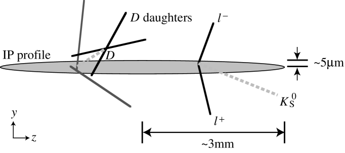
In this section, we describe the reconstruction of the proper-time interval between the decay points of the two $B$ mesons produced at KEKB. Figure 2 illustrates reconstruction of the decay vertices. The decay vertices of the two $B$ mesons in each event are fitted using tracks that have at least one three-dimensional coordinate determined from associated $r$-$\phi$ and $z$ hits in the same SVD layer plus one or more additional $z$ hits in other SVD layers. We impose the constraint that they are consistent with the interaction point (IP) profile, smeared in the $r$-$\phi$ plane by $21~{}\mu{\rm m}$ to account for the transverse $B$ decay length. The IP profile is described as a three-dimensional Gaussian, the parameters of which are determined in each run (in finer subdivisions, every 10,000 - 60, 000 events, for the mean position) using hadronic events. The size of the IP region is typically $\sigma_{x}\simeq 100~{}\mu{\rm m}$, $\sigma_{y}\simeq 5~{}\mu{\rm m}$, and $\sigma_{z}\simeq 3$ mm, where $x$ and $y$ denote the horizontal and vertical directions, respectively.

One $B$ meson is fully reconstructed in one of the following decay modes : ${\overline{B}{}^{0}}\to D^{+}\pi^{-}$, $D^{*+}\pi^{-}$, $D^{*+}\rho^{-}$, ${J/\psi}K_{S}^{0}$, ${J/\psi}\overline{K}{}^{*0}$, ${B^{-}}\to D^{0}\pi^{-}$, and ${J/\psi}K^{-}$, where ${J/\psi}$ is reconstructed via ${J/\psi}\to\ell^{+}\ell^{-}(\ell=e,\mu)$ decay, and $D^{*+}$ via $D^{*+}\to D^{0}\pi^{+}$ decay. Neutral and charged $D$ mesons are reconstructed in the following channels: $D^{0}\to K^{-}\pi^{+},K^{-}\pi^{+}\pi^{0},K^{-}\pi^{+}\pi^{+}\pi^{-}$, and $D^{+}\to K^{-}\pi^{+}\pi^{+}$. The details of the event selection can be found elsewhere [2].

In the case of a fully reconstructed $\overline{B}\to D^{(*)}X$ decay, the $B$ decay point is obtained from the vertex position and momentum vector of the reconstructed $D$ meson and tracks other than the slow $\pi^{+}$ candidate from $D^{*+}$ decay. For a fully reconstructed $\overline{B}\to{J/\psi}X$ decay, the $B$ vertex is determined using lepton tracks from the ${J/\psi}$.

The decay vertex of the associated $B$ meson is determined by applying a vertex-fit program to all tracks not assigned to the fully reconstructed $B$ meson; however, poorly reconstructed tracks (with a longitudinal position error in excess of $500~{}\mu{\rm m}$) as well as tracks that are likely to come from $K_{S}^{0}$ decays (forming the $K_{S}^{0}$ mass with another track, or emanating from a point more than $500~{}\mu{\rm m}$ away from the fully reconstructed $B$ vertex in the $r$-$\phi$ plane) are not used. If the reduced $\chi^{2}$ $(\chi^{2}/{\rm n.d.f.})$ associated with a found vertex exceeds 20, the track making the largest $\chi^{2}$ contribution is removed and the vertex is refitted. This procedure is repeated until $\chi^{2}/{\rm n.d.f.}<20$ is obtained or only one track is left. If, however, the track to be removed is a lepton with a cms momentum greater than 1.1 ${\rm GeV}/c$, we keep the lepton and remove the track making the second largest $\chi^{2}$ contribution. This is because high-momentum leptons are likely to come from primary semi-leptonic $B$ decays. The presence of a secondary charm $(b\to c)$ decay vertex in the associated $B$ meson results in a shift of the reconstructed vertex point toward the charm flight direction and degrades the vertex resolution. A Monte Carlo (MC) simulation study shows that the shift and the resolution of the associated $B$ decay vertex are $\sim 20$ $\mu{\rm m}$ and $\sim 140$ $\mu{\rm m}$ (rms), respectively, while the resolution of the fully reconstructed $B$ decay vertex is $\sim 75$ $\mu{\rm m}$ (rms).

Figure 2: Illustration of vertex reconstruction of two $B$ decay vertices.

Because of the IP profile constraint it is possible to reconstruct a decay vertex even with a single track. The fraction of single-track vertices is $\sim 10\%$ and $\sim 22\%$ for the fully reconstructed and associated $B$ decays, respectively. For the multiple-track vertices, the quality of the vertex fit, for both the fully reconstructed and associated $B$ meson decays, is further evaluated. Using MC simulation, we find that the vertex-fit $\chi^{2}$ is correlated with the $B$ decay length due to the tight IP constraint in the transverse plane. To avoid this correlation, we use the variable based on the $z$ information only (contrary to the vertex-fit $\chi^{2}$ calculated using three dimensional information):

$$\xi\equiv(1/2n)\sum^{n}_{i}\left[(z_{\rm after}^{i}-z_{\rm before}^{i})/\varepsilon_{\rm before}^{i}\right]^{2},$$ (1)

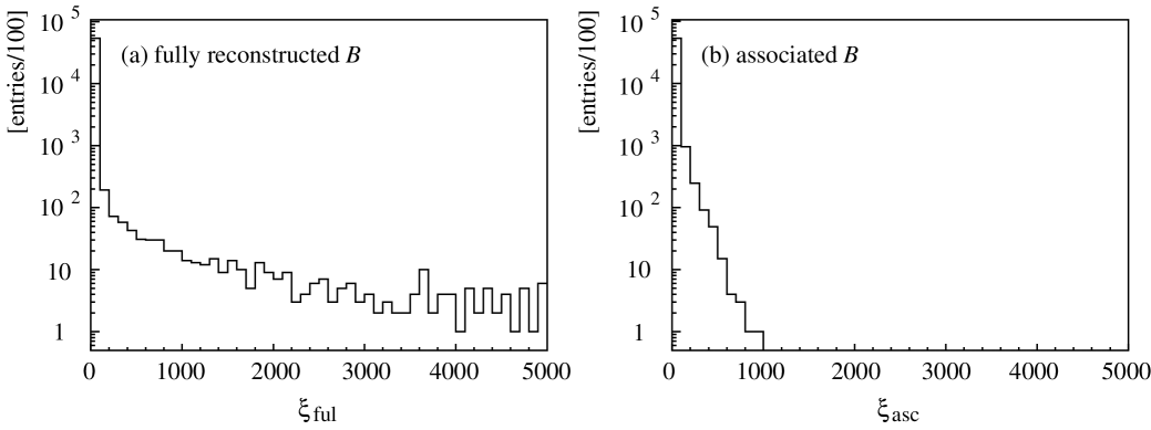
where $n$ is the number of tracks used in the fit , $z_{\rm before}^{i}$ and $z_{\rm after}^{i}$ are the $z$ positions of each track (at the closest approach to the origin) before and after the vertex fit, respectively, and $\varepsilon_{\rm before}^{i}$ is the error of $z_{\rm before}^{i}$. Figure 3 shows the $\xi$ distributions for the (a) fully reconstructed and (b) associated $B$ decay vertices, obtained using a MC simulation. Because the $\chi^{2}/{\rm n.d.f.}$ requirement is imposed on the associated $B$ decay vertices, the $\xi$ distribution for those vertices does not show an extended tail compared to that for the fully reconstructed $B$ decay vertices. Figure 4 shows the $\xi$ distributions as a function of the $B$ decay length for the (a) fully reconstructed and (b) associated $B$ decay vertices. As indicated, $\xi$ does not depend on the $B$ decay length. We require $\xi<100$ for both vertices to eliminate poorly reconstructed vertices. We find that about 3% of the fully reconstructed and 1% of the associated $B$ decay vertices are rejected in the data.

Figure 3: The $\xi$ distributions for the (a) fully reconstructed and (b) associated $B$ decays, obtained using $\overline{B}{}^{0}\to J/\psi K_{S}^{0}$ MC events.

Figure 4: Monte Carlo $\xi$ distribution as a function of the $B$ decay length, obtained for the (a) fully reconstructed and (b) associated $B$ decay vertices.

The proper-time interval between the fully-reconstructed and the associated $B$ decays is calculated as

$$\Delta t=(z_{\rm ful}-z_{\rm asc})/[c(\beta\gamma)_{\Upsilon}],$$ (2)

where $z_{\rm ful}$ and $z_{\rm asc}$ are the $z$ coordinates of the fully-reconstructed and associated $B$ decay vertices, respectively. We reject a small fraction ($\sim$0.2%) of the events by requiring $|\Delta t|<70$ ps ($\sim$45$\tau_{B}$).

4 Resolution function

4.1 Overview

We extract the lifetimes of $B$ mesons using an unbinned maximum likelihood fit to the observed $\Delta t$ distributions. We maximize the likelihood function $L=\prod_{i}P(\Delta t_{i})$, where $P(\Delta t_{i})$ is the probability density function (PDF) for the $\Delta t$ of the $i$-th event and the product is taken over all the selected events.

The function $P(\Delta t)$, expressed as

$$P(\Delta t)=(1-f_{{\rm ol}})\left[f_{{\rm sig}}P_{{\rm sig}}(\Delta t)+(1-f_{{\rm sig}})P_{{\rm bkg}}(\Delta t)\right]+f_{{\rm ol}}P_{{\rm ol}}(\Delta t),$$ (3)

contains contributions from the signal and the background ($P_{{\rm sig}}$ and $P_{{\rm bkg}}$), where $f_{{\rm sig}}$ is the signal purity determined on an event-by-event basis, $P_{{\rm sig}}$ is described as the convolution of a true PDF ($\mathcal{P}_{{\rm sig}}$) with a resolution function ($R_{{\rm sig}}$) and $P_{{\rm bkg}}$ is expressed in a similar way:

$$P_{\rm sig(bkg)}(\Delta t)=\int_{-\infty}^{+\infty}\d(\Delta t^{\prime}){\mathcal{P}}_{\rm sig(bkg)}(\Delta t^{\prime})R_{\rm sig(bkg)}(\Delta t-\Delta t^{\prime}).$$ (4)

To account for a small number of events that give large $\Delta t$ in both the signal and background (outlier components), we introduce a fraction of outliers ($f_{{\rm ol}}$) and a Gaussian function ($P_{{\rm ol}}(\Delta t)$) to model its distribution. The true PDF for the signal, $\mathcal{P}_{{\rm sig}}(\Delta t;\tau_{B})$, is given by

$$\mathcal{P}_{{\rm sig}}(\Delta t;\tau_{B})=\frac{1}{2\tau_{B}}\exp\left(-\frac{|\Delta t|}{\tau_{B}}\right),$$ (5)

where $\tau_{B}$ is, depending on the reconstructed mode in the event, either the $\overline{B}{}^{0}$ or the $B^{-}$ lifetime. The signal PDFs for the measurements of the $B^{0}\overline{B}{}^{0}$ oscillation frequency and the time-dependent $CP$ asymmetry are given in Section 5.

The resolution function of the signal is constructed as the convolution of four different contributions: the detector resolution on $z_{\rm ful}$ and $z_{\rm asc}$ ($R_{{\rm ful}}$ and $R_{{\rm asc}}$), an additional smearing on $z_{\rm asc}$ due to the inclusion of tracks which do not originate from the associated $B$ vertex ($R_{{\rm np}}$), mostly due to charm and $K_{S}^{0}$ decays, and the kinematic approximation that the $B$ mesons are at rest in the cms ($R_{{\rm k}}$). The overall resolution function, $R_{{\rm sig}}(\Delta t)$, is expressed as

$$R_{{\rm sig}}(\Delta t) = \int\!\!\!\int\!\!\!\int_{-\infty}^{+\infty}\mathrm{d}(\Delta t^{\prime})\,\mathrm{d}(\Delta t^{\prime\prime})\,\mathrm{d}(\Delta t^{\prime\prime\prime})\,R_{{\rm ful}}(\Delta t-\Delta t^{\prime})R_{{\rm asc}}(\Delta t^{\prime}-\Delta t^{\prime\prime})$$ (6)

$$\times R_{{\rm np}}(\Delta t^{\prime\prime}-\Delta t^{\prime\prime\prime})R_{{\rm k}}(\Delta t^{\prime\prime\prime}).$$

We use a MC simulation to understand the resolution function and determine its functional form. The MC events are generated using the QQ event generator [7] and the response of the Belle detector is modeled by a GEANT3-based full-simulation program [8]. One of $B$ mesons in each event is forced to decay to ${J/\psi}K_{S}^{0}$, ${J/\psi}K^{-}$ or $D\pi$ while the other decays generically to one of all possible final states.

4.2 Detector resolution

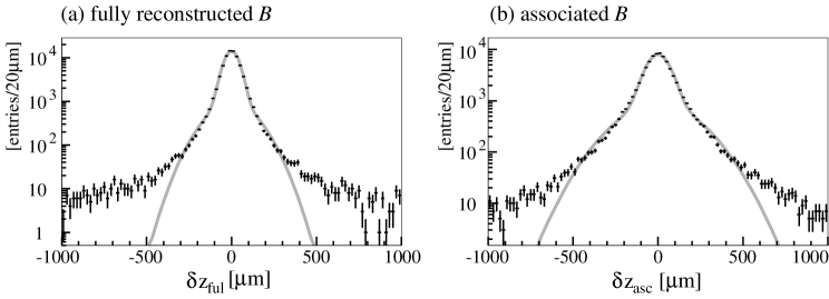
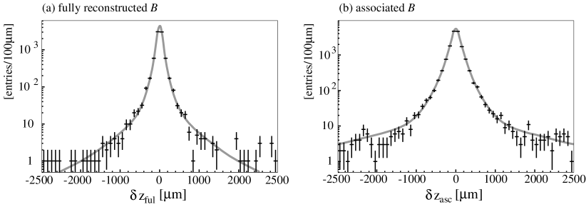
The detector resolution ($R_{{\rm ful}}$ and $R_{{\rm asc}}$) is studied using a special MC simulation in which all short-lived ($\tau<10^{-9}$ s) secondary particles (including $K_{S}^{0}$ and $\Lambda$) are forced to decay with zero lifetime at the $B$ meson decay points. Figures 5 (a) and (b) show the distributions of the difference in $z$ between the reconstructed and generated vertex positions:

$$\delta z_{q}=z_{q}^{\rm rec}-z_{q}^{\rm gen},$$ (7)

where $q={\rm ful}({\rm asc})$ is for the fully reconstructed (associated) $B$ vertex, and the superscripts ‘rec’ and ‘gen’ denote the reconstructed and generated vertex positions, respectively. Results of the fit to a sum of two Gaussians are also shown. The fitted curves do not represent the $\delta z$ distributions in the tail regions. We also find that even a sum of three or more Gaussians with constant standard deviations cannot represent $\delta z$ properly. We therefore consider a more elaborate function that uses the vertex-by-vertex $z$-coordinate error of the reconstructed vertex, $\sigma^{z}_{q}$ ($q$ = full, asc), as an input parameter. The value of $\sigma^{z}_{q}$ is computed from the error matrix of the tracks used in the vertex fit and the size of the IP region. To construct functional forms of $R_{{\rm ful}}$ and $R_{{\rm asc}}$ we investigate the distribution of a pull, defined as $\delta z_{q}$ divided by $\sigma^{z}_{q}$. If the $\sigma^{z}_{q}$ estimation is correct on average, the pull distribution is expected to be a single Gaussian with the standard deviation of unity.

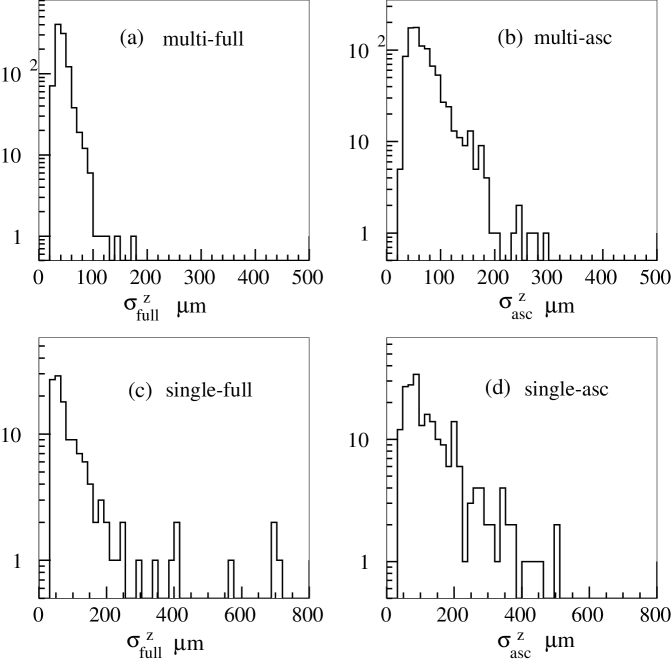
Because the resolution for the multiple-track vertices is better than that for the single-track vertices, we consider them separately. Figure 6 shows the distributions of $\sigma^{z}_{\rm full}$ and $\sigma^{z}_{\rm asc}$ for the multi-track and single-track vertices obtained from $B^{0}\to J/\psi K_{S}^{0}$ data.

Figure 5: The $\delta z$ distributions of the (a) fully reconstructed and (b) associated $B$ vertices obtained from a ${\overline{B}{}^{0}}\to{J/\psi}K_{S}^{0}$ MC sample. Superimposed are the results of a fit to the sum of two Gaussians.

Figure 6: Distributions of the vertex-by-vertex $z$-coordinate error $\sigma^{z}$ of the (a) (b) mutli-track and (c) (d) single-track vertices for the fully reconstructed and associated $B$ decays, obtained from $\overline{B^{0}}\to J/\psi K_{S}^{0}$ data.

4.2.1 Multiple-track vertex

We investigate the vertex fit quality dependence of the resolution using the value of $\xi$ defined in Eq. (1). We find that a pull distribution for vertices with similar $\xi$ values can be expressed as a single Gaussian. Furthermore, we find that the standard deviation of the distribution has a linear dependence on $\xi$ as shown in Fig. 7.

Figure 7: Standard deviations of the pull distributions as a function of $\xi$ for (a) the fully reconstructed and (b) the associated $B$ meson vertices. The distributions are obtained from a ${\overline{B}{}^{0}}\to{J/\psi}K_{S}^{0}$ MC sample.

Results from this MC study lead us to model the detector resolution of the multiple-track vertex using the following function:

$$R_{q}^{\rm multiple}(\delta z_{q})=G(\delta z_{q};(s_{q}^{0}+s_{q}^{1}\xi)\sigma^{z}_{q})\,\ (q={\rm ful,\ asc}),$$ (8)

where $G$ is the Gaussian function,

$$G(x;\sigma)\equiv\frac{1}{\sqrt{2\pi}\sigma}\exp\left(-\frac{x^{2}}{2\sigma^{2}}\right).$$ (9)

The scale factors $s_{q}^{0}$ and $s_{q}^{1}$ are treated as free parameters and determined from the lifetime fit to the data.

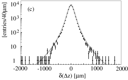
Figure 8: Distributions of (a) $\delta z_{\rm ful}$ and (b) $\delta z_{\rm asc}$ for multiple-track vertices, with $R_{{\rm ful}}^{\rm multiple}(\delta z_{\rm ful})$ and $R_{{\rm asc}}^{\rm multiple}(\delta z_{\rm asc})$, respectively. Figure (c) is the $\delta(\Delta z)$ distribution, and the convolution of $R_{{\rm ful}}^{\rm multiple}(\delta z_{\rm ful})$ and $R_{{\rm asc}}^{\rm multiple}(\delta z_{\rm asc})$.

Figures 8 (a) and (b) show the $\delta z_{\rm ful}$ and $\delta z_{\rm asc}$ distributions, respectively. Superimposed are the curves obtained by summing vertex-by-vertex $R_{q}^{\rm multiple}(\delta z_{q})$ functions. The curves well reproduce the $\delta z_{q}$ distributions. This demonstrates that $R_{q}^{\rm multiple}$ represents the detector resolution better than the sum of two Gaussians in Fig. 5. Figure 8 (c) shows the distribution of the residual of $\Delta z$, $\delta(\Delta z)\equiv\Delta z^{\rm rec}-\Delta z^{\rm gen}$ together with the convolution of $R_{{\rm ful}}^{\rm multiple}(\delta z_{\rm ful})$ and $R_{{\rm asc}}^{\rm multiple}(\delta z_{\rm asc})$.

4.2.2 Single-track vertex

For the single-track vertices, $\xi$ is not available. The resolution function of the single-track vertices, $R_{q}^{\rm single}(\delta z_{q})\ (q={\rm ful,\ asc})$, is expressed as a sum of two Gaussians, one for the main part of the detector resolution and the other for the tail part, which is due to poorly reconstructed tracks:

$$R_{q}^{\rm single}(\delta z_{q})=(1-f_{\rm tail})G(\delta z_{q};s_{\rm main}\sigma_{q}^{z})+f_{\rm tail}G(\delta z_{q};s_{\rm tail}\sigma_{q}^{z}),$$ (10)

where $s_{\rm main}$ and $s_{\rm tail}$ are global scale factors which are common to all single-track vertices. Figure 9 shows the residual distributions of the single-track $z_{\rm ful}$ and $z_{\rm asc}$ vertices, together with a fit to $R_{q}^{\rm single}(\delta z_{q})$.

Figure 9: The (a) $\delta z_{\rm ful}$ and (b) $\delta z_{\rm asc}$ distributions for single-track vertices with $R_{{\rm ful}}^{\rm single}$ and $R_{{\rm asc}}^{\rm single}.$

4.3 Smearing due to non-primary tracks

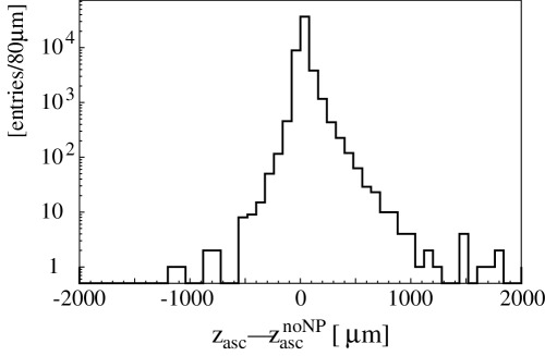
We introduce another resolution function, $R_{{\rm np}}$, to represent the smearing of $z_{\rm asc}$ due to tracks that do not originate from the associated $B$ vertex consists of a prompt component, expressed by Dirac’s $\delta$-function $\delta^{\rm Dirac}(\delta z_{\rm asc})$, and components that account for smearing due to $K_{S}^{0}$ and charm decays. The functional form of the non-prompt components is determined from the difference between $z_{\rm asc}$ obtained for the nominal MC sample and that for the special MC sample in which all short-lived secondary particles are forced to decay with zero lifetime at the $B$ decay points, shown in Fig. 10. It can be expressed by a function defined as $f_{\mathrm{p}}E_{\mathrm{p}}(\delta z_{\rm asc};\tau_{\rm np}^{\mathrm{p}})+(1-f_{\mathrm{p}})E_{\mathrm{n}}(\delta z_{\rm asc};\tau_{\rm np}^{\mathrm{n}}),$ where $f_{\mathrm{p}}$ is a fraction of the $\delta z_{\rm asc}>0$ component and $E_{\mathrm{p}}$ and $E_{\mathrm{n}}$ are:

$$E_{\mathrm{p}}(x;\tau) \equiv \frac{1}{\tau}\exp\left(-\frac{x}{\tau}\right){\rm for}\ x>0,{\rm otherwise}\ 0,$$ (11)

$$E_{\mathrm{n}}(x;\tau) \equiv \frac{1}{\tau}\exp\left(+\frac{x}{\tau}\right){\rm for}\ x\leq 0,\ {\rm otherwise}\ 0.$$ (12)

Thus, $R_{{\rm np}}$ is given by

$$R_{{\rm np}}(\delta z_{\rm asc})\equiv f_{\delta}\delta^{\rm Dirac}(\delta z_{\rm asc})+(1-f_{\delta})\left[f_{\mathrm{p}}E_{\mathrm{p}}(\delta z_{\rm asc};\tau_{\rm np}^{\mathrm{p}})+(1-f_{\mathrm{p}})E_{\mathrm{n}}(\delta z_{\rm asc};\tau_{\rm np}^{\mathrm{n}})\right],$$ (13)

where $f_{\delta}$ is the prompt-component fraction.

Figure 10: Distribution of $z_{\rm asc}-z_{\rm asc}^{\rm noNP}$ for multi-track vertices, where $z_{\rm asc}^{\rm noNP}$ is $z_{\rm asc}$ obtained from a MC sample in which secondary decays are turned off. In making this plot the events in which $z_{\rm asc}^{\rm noNP}=z_{\rm asc}$ are removed. The histogram is obtained from ${\overline{B}{}^{0}}\to{J/\psi}K_{S}^{0}$ MC whose associated $B$ vertex is reconstructed with multiple tracks.

We find that the vertex position shift has linear dependence on both $\sigma^{z}_{\rm asc}$ and $\xi^{z}_{\rm asc}$ as shown in Fig. 11 for multi-track vertices. Consequently, we assume $\tau_{\rm np}^{\mathrm{p}}$ and $\tau_{\rm np}^{\mathrm{n}}$ are bilinear with $\sigma_{\rm asc}$ and $\xi_{\rm asc}$ as

$$\tau_{\rm np}^{\mathrm{p}} = \tau_{\mathrm{p}}^{0}+\tau_{\mathrm{p}}^{1}(s_{\rm asc}^{0}+s_{\rm asc}^{1}\xi^{z}_{\rm asc})\sigma^{z}_{\rm asc}/c(\beta\gamma)_{\Upsilon},\ \ {\rm and}$$ (14)

$$\tau_{\rm np}^{\mathrm{n}} = \tau_{\mathrm{n}}^{0}+\tau_{\mathrm{n}}^{1}(s_{\rm asc}^{0}+s_{\rm asc}^{1}\xi_{\rm asc})\sigma^{z}_{\rm asc}/c(\beta\gamma)_{\Upsilon}.$$ (15)

Figure 11: Average shift of vertex position ($z_{\rm asc}-z_{\rm asc}^{\rm noNP}$) vs (a) $\sigma^{z}_{\rm asc}$ and (b) $\xi_{\rm asc}$. $z_{\rm asc}^{\rm noNP}$ is obtained from a MC sample in which secondary decays are turned off. The events with $z_{\rm asc}<z_{\rm asc}^{\rm noNP}$ are excluded.

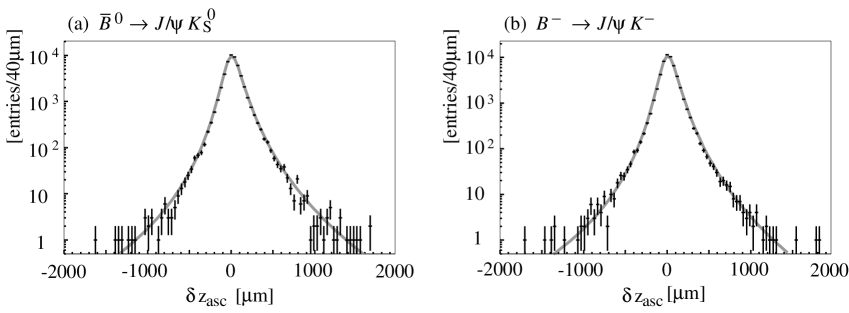
Figure 12: The $\delta z_{\rm asc}$ distributions of multiple-track vertices for (a) ${\overline{B}{}^{0}}\to{J/\psi}K_{S}^{0}$ and (b) ${B^{-}}\to{J/\psi}K^{-}$ decays.

We determine six parameters in $R_{{\rm np}}$, $f_{\delta}$, $f_{\mathrm{p}}$, $\tau_{\mathrm{p}}^{0}$, $\tau_{\mathrm{p}}^{1}$, $\tau_{\mathrm{n}}^{0}$, and $\tau_{\mathrm{n}}^{1}$ by fitting the convolution of $R_{{\rm asc}}^{\rm multiple}$ and $R_{{\rm np}}$ to the $\delta z_{\rm asc}$ distributions for $\overline{B}{}^{0}$ and $B^{-}$ separately, as shown in Fig. 12. In this fit, the scale parameters, $s^{0}_{\rm asc}$ and $s^{1}_{\rm asc}$, for $R_{{\rm asc}}^{\rm multiple}$ are fixed to the values (common to $\overline{B}{}^{0}$ and $B^{-}$) obtained by fitting $R_{{\rm asc}}^{\rm multiple}$ to the special MC sample (in which all short-lived secondary particles are forced to decay promptly at the $B$ meson decay points). Results, shown superimposed, well represent the distributions.

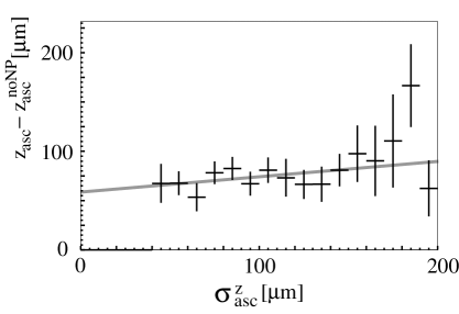
For single-track vertices we consider the correlation between the vertex position shift and $\sigma^{z}_{\rm asc}$. Figure 13 shows the vertex position shift versus $\sigma^{z}_{\rm asc}$ for the single-track vertices.

Figure 13: Average shift of vertex positions ($z_{\rm asc}-z_{\rm asc}^{\rm noNP}$) versus $\sigma^{z}_{\rm asc}$ for single-track vertices. The events where $z_{\rm asc}<z_{\rm asc}^{\rm noNP}$ are excluded.

Since $R_{{\rm asc}}$ for the single-track vertices is defined as a sum of main and tail Gaussians, we also introduce $R_{{\rm np}}^{\rm main}$ and $R_{{\rm np}}^{\rm tail}$ for main and tail parts, respectively. Each of $R_{{\rm np}}^{\rm main}$ and $R_{{\rm np}}^{\rm tail}$ is expressed by the function of Eq. (13) with parameters defined as:

$$(\tau_{\rm np}^{\mathrm{p}})_{\rm main} = \tau_{\mathrm{p}}^{0}+\tau_{\mathrm{p}}^{1}s_{\rm main}\sigma^{z}_{\rm asc}/c(\beta\gamma)_{\Upsilon}$$

$$(\tau_{\rm np}^{\mathrm{n}})_{\rm main} = \tau_{\mathrm{n}}^{0}+\tau_{\mathrm{n}}^{1}s_{\rm main}\sigma^{z}_{\rm asc}/c(\beta\gamma)_{\Upsilon},$$ (16)

$$(\tau_{\rm np}^{\mathrm{p}})_{\rm tail\ \ } = \tau_{\mathrm{p}}^{0}+\tau_{\mathrm{p}}^{1}s_{\rm tail}\sigma^{z}_{\rm asc}/c(\beta\gamma)_{\Upsilon},\ \ {\rm and}$$

$$(\tau_{\rm np}^{\mathrm{n}})_{\rm tail\ \ } = \tau_{\mathrm{n}}^{0}+\tau_{\mathrm{n}}^{1}s_{\rm tail}\sigma^{z}_{\rm asc}/c(\beta\gamma)_{\Upsilon}.$$ (17)

The convolution of $R_{{\rm asc}}$ and $R_{{\rm np}}$ for single-track vertices is, thus, defined as:

$$R_{{\rm asc}}^{\rm single}\otimes R_{{\rm np}}^{\rm single}(\delta z_{\rm asc}) = \int_{-\infty}^{+\infty}\mathrm{d}(\delta z_{\rm asc}^{\prime})\left[(1-f_{\rm tail})G(\delta z_{\rm asc}-\delta z_{\rm asc}^{\prime};s_{\rm main}\sigma_{q})R_{{\rm np}}^{\rm main}(\delta z_{\rm asc}^{\prime})\right]$$ (18)

$$+ \int_{-\infty}^{+\infty}\mathrm{d}(\delta z_{\rm asc}^{\prime})\left[f_{\rm tail}G(\delta z_{\rm asc}-\delta z_{\rm asc}^{\prime};s_{\rm tail}\sigma_{q})R_{{\rm np}}^{\rm tail}(\delta z_{\rm asc}^{\prime})\right].$$

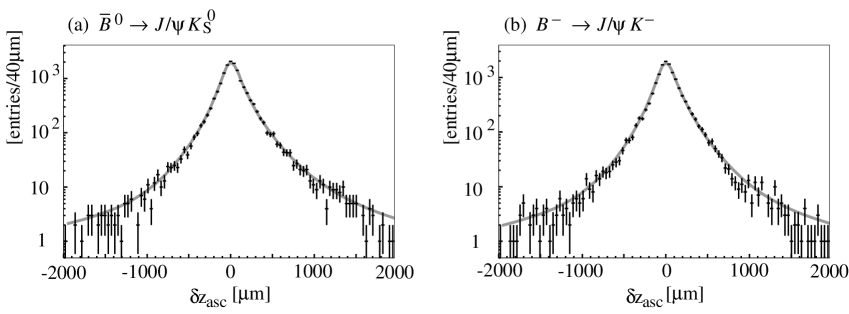
Figure 14 shows the $\delta z_{\rm asc}$ distributions for the single track vertices. The superimposed curves are the results of a fit to the function given by Eq. (18).

Figure 14: The $\delta z_{\rm asc}$ distributions of single-track vertices for (a) $\overline{B}{}^{0}$ and (b) $B^{-}$ mesons.

Table 1 lists the shape parameters of $R_{{\rm np}}$ determined by fitting $R_{{\rm asc}}\otimes R_{{\rm np}}(\delta z_{\rm asc})$ to MC $\delta z_{\rm asc}$ distributions. These parameter values are held fixed when the lifetime fit to the data is performed.

Table 1: Shape parameters of $R_{{\rm np}}$ used for the lifetime fit. The values are determined for multiple- and single-track vertices, separately, using Monte Carlo $\delta z_{\rm asc}$ distributions.

	${\overline{B}{}^{0}}$			${B^{-}}$
	multiple	single		multiple	single
$f_{\delta}$	$0.676\pm 0.007$	$0.787\pm 0.011$		$0.650\pm 0.010$	$0.763\pm 0.018$
$f_{\mathrm{p}}$	$0.955\pm 0.004$	$0.790\pm 0.021$		$0.963\pm 0.004$	$0.757\pm 0.026$
$\tau_{\mathrm{p}}^{0}$ (ps )	$-0.010\pm 0.011$	$0.108\pm 0.068$		$0.037\pm 0.012$	$-0.019\pm 0.066$
$\tau_{\mathrm{p}}^{1}$	$0.927\pm 0.025$	$1.321\pm 0.097$		$0.674\pm 0.025$	$1.113\pm 0.096$
$\tau_{\mathrm{n}}^{0}$ (ps)	$-0.194\pm 0.078$	$-0.281_{-0.147}^{+0.130}$		$-0.269\pm 0.099$	$-0.375_{-0.122}^{+0.111}$
$\tau_{\mathrm{n}}^{1}$	$1.990_{-0.169}^{+0.182}$	$1.583_{-0.184}^{+0.213}$		$2.070_{-0.213}^{+0.235}$	$1.548_{-0.182}^{+0.207}$

4.4 Kinematic approximation

The proper time interval calculated as Eq. (2) , $\Delta t=(z_{\rm ful}-z_{\rm asc})/[c(\beta\gamma)_{\Upsilon}]$, is equal to the true proper-time interval when the cms motion of the $B$ mesons is neglected. The difference between $\Delta t$ and the true proper-time interval $\Delta t_{\rm true}=t_{\rm ful}-t_{\rm asc}$ is calculated from the kinematics of the $\Upsilon(4S)$ two-body decay:

$$x\equiv\Delta t-\Delta t_{\rm true} = (z_{\rm ful}-z_{\rm asc})/[c(\beta\gamma)_{\Upsilon}]-(t_{\rm ful}-t_{\rm asc})$$ (19)

$$= [t_{\rm ful}c(\beta\gamma)_{\rm ful}-t_{\rm asc}c(\beta\gamma)_{\rm asc}]/[c(\beta\gamma)_{\Upsilon}]-(t_{\rm ful}-t_{\rm asc})$$

$$= [(\beta\gamma)_{\rm ful}/(\beta\gamma)_{\Upsilon}-1]t_{\rm ful}-[(\beta\gamma)_{\rm asc}/(\beta\gamma)_{\Upsilon}-1]t_{\rm asc},$$

where $(\beta\gamma)_{\rm ful}$ and $(\beta\gamma)_{\rm asc}$ are Lorentz boost factors of the fully reconstructed and associated $B$ mesons, respectively, and their ratios to $(\beta\gamma)_{\Upsilon}$ are given as:

$$(\beta\gamma)_{\rm ful}/(\beta\gamma)_{\Upsilon} = \frac{E_{B}^{{\rm cms}}}{m_{B}}+\frac{p_{B}^{{\rm cms}}\cos{\theta_{B}^{{\rm cms}}}}{\beta_{\Upsilon}m_{B}}\sim 1+0.165\cos{\theta_{B}^{{\rm cms}}},\ \ {\rm and}$$ (20)

$$(\beta\gamma)_{\rm asc}/(\beta\gamma)_{\Upsilon} = \frac{E_{B}^{{\rm cms}}}{m_{B}}-\frac{p_{B}^{{\rm cms}}\cos{\theta_{B}^{{\rm cms}}}}{\beta_{\Upsilon}m_{B}}\sim 1-0.165\cos{\theta_{B}^{{\rm cms}}},$$ (21)

where $\beta_{\Upsilon}=0.391$ is the velocity of the $\Upsilon(4S)$ in units of $c$, $E_{B}^{\rm cms}\sim 5.292~{}{\rm GeV}$, $p_{B}^{\rm cms}\sim 0.340~{}{\rm GeV}/c$ and $\theta_{B}^{\rm cms}$ are the energy, momentum and polar angle of the fully reconstructed $B$ in the cms, and $m_{B}$ is either the $\overline{B}{}^{0}$ or the $B^{-}$ mass. The difference $x$ can, therefore, be approximated as

$$x\sim 0.165\cos{\theta_{B}^{{\rm cms}}}(t_{\rm ful}+t_{\rm asc}).$$ (22)

$R_{{\rm k}}$, which accounts for $x$, can be given as a function of $\cos\theta_{B}^{\rm cms}$. Because $t_{\rm ful}$ and $t_{\rm asc}$ distributions follow $E_{\mathrm{p}}(t_{\rm ful};\tau_{B})=\frac{1}{\tau_{B}}\exp(-t_{\rm ful}/\tau_{B})$ and $E_{\mathrm{p}}(t_{\rm asc};\tau_{B})=\frac{1}{\tau_{B}}\exp(-t_{\rm asc}/\tau_{B})$, respectively, the probability density of obtaining $x$ and $\Delta t_{\rm true}$ simultaneously is given by:

$$F(x,\Delta t_{\rm true}) = \int_{0}^{\infty}\int_{0}^{\infty}\mathrm{d}t_{\rm ful}\mathrm{d}t_{\rm asc}E_{\mathrm{p}}(t_{\rm ful};\tau_{B})E_{\mathrm{p}}(t_{\rm asc};\tau_{B})\delta^{\rm Dirac}(\Delta t_{\rm true}-(t_{\rm ful}-t_{\rm asc}))$$

$$\times\delta^{\rm Dirac}(x-\{[(\beta\gamma)_{\rm ful}/(\beta\gamma)_{\Upsilon}-1]t_{\rm ful}-[(\beta\gamma)_{\rm asc}/(\beta\gamma)_{\Upsilon}-1]t_{\rm asc}\}),$$

and the probability density of obtaining $\Delta t_{\rm true}$ is given by:

$$F(\Delta t_{\rm true})=\int_{0}^{\infty}\int_{0}^{\infty}\mathrm{d}t_{\rm ful}\mathrm{d}t_{\rm asc}E_{\mathrm{p}}(t_{\rm ful};\tau_{B})E_{\mathrm{p}}(t_{\rm asc};\tau_{B})\delta^{\rm Dirac}(\Delta t_{\rm true}-(t_{\rm ful}-t_{\rm asc})).$$ (24)

$R_{{\rm k}}(x)$ is, then, defined as the conditional probability density of obtaining $x$ given $\Delta t_{\rm true}$. It is expressed as $R_{{\rm k}}(x)=F(x,\Delta t_{\rm true})/F(\Delta t_{\rm true})$ which gives:

$$R_{{\rm k}}(x)=\begin{cases}E_{\mathrm{p}}\left(x-\Bigl{[}(\frac{E_{B}^{{\rm cms}}}{m_{B}}-1)\Delta t_{\rm true}+\frac{p_{B}^{{\rm cms}}\cos{\theta_{B}^{{\rm cms}}}}{\beta_{\Upsilon}m_{B}}|\Delta t_{\rm true}|\Bigr{]};|\frac{p_{B}^{{\rm cms}}\cos{\theta_{B}^{{\rm cms}}}}{\beta_{\Upsilon}m_{B}}|\tau_{B}\right)&(\cos\theta_{B}^{\rm cms}>0)\\ \delta^{\rm Dirac}\left(x-(\frac{E_{B}^{{\rm cms}}}{m_{B}}-1)\Delta t_{\rm true}\right)&(\cos\theta_{B}^{\rm cms}=0)\\ E_{\mathrm{n}}\left(x-\Bigl{[}(\frac{E_{B}^{{\rm cms}}}{m_{B}}-1)\Delta t_{\rm true}+\frac{p_{B}^{{\rm cms}}\cos{\theta_{B}^{{\rm cms}}}}{\beta_{\Upsilon}m_{B}}|\Delta t_{\rm true}|\Bigr{]};|\frac{p_{B}^{{\rm cms}}\cos{\theta_{B}^{{\rm cms}}}}{\beta_{\Upsilon}m_{B}}|\tau_{B}\right)&(\cos\theta_{B}^{\rm cms}<0)\end{cases}.$$ (25)

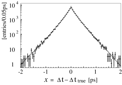
Figure 15 shows the $x$ distribution for $\overline{B}{}^{0}\to J/\psi K_{S}^{0}$ events with the function $R_{{\rm k}}(x)$. The expected theoretical $\Delta t$ distribution $P(\Delta t)$ can be expressed as a convolution of the true PDF $\mathcal{P}_{{\rm sig}}(\Delta t_{\rm true};\tau_{B})$ with $R_{{\rm k}}(\Delta t-\Delta t_{\rm true})$:

$$P(\Delta t)=\frac{m_{B}}{2E_{B}^{{\rm cms}}\tau_{B}}\exp\left(-\frac{|\Delta t|}{(\frac{E_{B}^{{\rm cms}}}{m_{B}}\pm\frac{p_{B}^{{\rm cms}}\cos{\theta_{B}^{{\rm cms}}}}{\beta_{\Upsilon}m_{B}})\tau_{B}}\right)\qquad\begin{cases}+\ {\rm for}\ \Delta t\geq 0\\ -\ {\rm for}\ \Delta t<0\end{cases}.$$ (26)

Figure 15: The $x=\Delta t-\Delta t_{\rm true}$ distribution for $\overline{B}{}^{0}\to J/\psi K_{S}^{0}$ events together with the function $R_{{\rm k}}(x)$.

4.5 Background distribution

The signal purity $f_{\rm sig}$ in Eq. (3) is determined on an event-by-event basis as a function of two kinematic variables, the energy difference $\Delta E=E_{B}^{\rm cms}-E_{\rm beam}^{\rm cms}$ and the beam-energy constrained mass $M_{\rm bc}=\sqrt{(E_{\rm beam}^{\rm cms})^{2}-(p_{B}^{\rm cms})^{2}}$, where $E_{\rm beam}^{\rm cms}$ is the beam energy in the cms. Typical $f_{\rm sig}$ values for the decay modes used for the measurement of $B$ meson lifetimes and $B^{0}\overline{B}{}^{0}$ oscillation frequency are listed in Table 2. The values listed are obtained for the signal region defined as $|M_{\rm bc}-m_{B}|<3\sigma.$ The composition of the background is studied by a MC simulation and is listed in Table 3. The largest contribution is from $c\bar{c}$ events produced in the continuum, while other continuum events ($u,d,s$ events) and combinatorial backgrounds from $B\overline{B}$ events also contribute.

Table 2: Typical values of the signal purity $f_{\rm sig}$ for the decay modes used for the measurement of $B$ meson lifetimes and $B^{0}\overline{B}{}^{0}$ oscillation frequency.

Decay mode $B_{\rm ful}$	Signal purity $f_{\rm sig}$
$\overline{B}{}^{0}\rightarrow D^{+}\pi^{-}$	0.861
$\overline{B}{}^{0}\rightarrow D^{*+}\pi^{-}$	0.812
$\overline{B}{}^{0}\rightarrow D^{*+}\rho^{-}$	0.699
$\overline{B}{}^{0}\rightarrow J/\psi K_{S}^{0}$	0.940
$\overline{B}{}^{0}\rightarrow J/\psi K^{*0}$	0.948
$B^{-}\rightarrow D^{0}\pi^{-}$	0.699
$B^{-}\rightarrow J/\psi K^{-}$	0.955

Table 3: The composition of the background in the decay modes used for the measurement of $B$ meson lifetimes and $B^{0}\overline{B}{}^{0}$ oscillation frequency. The sources of the backgrounds are the continuum production of $u\bar{u},d\bar{d},s\bar{s}$ pairs ($q\bar{q}(u,,d,s)$) and $c\bar{c}$ pairs ($q\bar{q}(c))$, and combinatorial backgrounds from $B^{+}B^{-}$ and $B^{0}\overline{B}{}^{0}$ events. $\overline{B}\rightarrow J/\psi X$ modes, in which the background fraction is very small, are not listed.

Decay mode $B_{\rm ful}$	$q\bar{q}(u,d,s)$	$q\bar{q}(c)$	$B^{+}B^{-}$	$B^{0}\overline{B}{}^{0}$
$\overline{B}{}^{0}\rightarrow D^{+}\pi^{-}$	0.25	0.40	0.21	0.14
$\overline{B}{}^{0}\rightarrow D^{*+}\pi^{-}$	0.10	0.48	0.24	0.18
$\overline{B}{}^{0}\rightarrow D^{*+}\rho^{-}$	0.10	0.43	0.26	0.21
$B^{-}\rightarrow D^{0}\pi^{-}$	0.29	0.45	0.17	0.09

The background PDF, $P_{{\rm bkg}}(\Delta t)$, is modeled as a sum of exponential and prompt components ($\mathcal{P}_{\rm bkg}(\Delta t)$) convolved with $R_{{\rm bkg}}(\Delta t)$:

$$P_{{\rm bkg}}(\Delta t)=\int^{+\infty}_{-\infty}{\rm d}(\Delta t^{\prime})\mathcal{P}_{\rm bkg}(\Delta t^{\prime})R_{{\rm bkg}}(\Delta t-\Delta t^{\prime}),$$ (27)

where

$$\mathcal{P}_{\rm bkg}(\Delta t)=f_{\delta}^{\rm bkg}\delta^{\rm Dirac}(\Delta t-\mu_{\delta}^{\rm bkg})+(1-f_{\delta}^{\rm bkg})\frac{1}{2\tau_{\rm bkg}}\exp\left(-\frac{|\Delta t-\mu_{\tau}^{\rm bkg}|}{\tau_{\rm bkg}}\right)$$ (28)

with $\mu_{\delta}^{\rm bkg}$ and $\mu_{\tau}^{\rm bkg}$ being offsets of the distribution, and

$$R_{{\rm bkg}}(\Delta t)=(1-f_{\rm tail}^{\rm bkg})G(\Delta t;s_{\rm main}^{\rm bkg}\sqrt{\sigma_{\rm ful}^{2}+\sigma_{\rm asc}^{2}})+f_{\rm tail}^{\rm bkg}G(\Delta t;s_{\rm tail}^{\rm bkg}\sqrt{\sigma_{\rm ful}^{2}+\sigma_{\rm asc}^{2}}).$$ (29)

Different values are used for $s_{\rm main}^{\rm bkg}$, $s_{\rm tail}^{\rm bkg}$, and $f_{\rm tail}^{\rm bkg}$ depending on whether both vertices are reconstructed with multiple tracks or not. All parameters in $P_{{\rm bkg}}(\Delta t)$ are determined by the fit to the $\Delta t$ distribution of the background-enhanced control sample (i.e. events in the sideband region of the $\Delta E$ or $M_{\rm bc}$ distribution). Table 4 lists the values obtained separately for each decay mode used in the lifetime fit.

Table 4: The background shape parameters obtained by fitting $P_{\rm bkg}(\Delta t)$ to the background-enhanced control sample.

(a) $\overline{B}\to J/\psi\overline{K}$ modes
Parameter	${\overline{B}{}^{0}}\to{J/\psi}K_{S}^{0}$	${\overline{B}{}^{0}}\to{J/\psi}\overline{K}{}^{*0}$	${B^{-}}\to{J/\psi}K^{-}$
$(s_{\rm main}^{{\rm bkg}})_{\text{multiple}}$	$0.40\pm 0.12$	$1.09\pm 0.25$	$0.79\pm 0.23$
$(s_{\rm tail}^{{\rm bkg}})_{\text{multiple}}$	$9.46^{+4.26}_{-2.57}$	$6.97^{+6.39}_{-2.30}$	$1.90^{+0.64}_{-0.37}$
$(f_{\rm tail}^{{\rm bkg}})_{\text{multiple}}$	$0.29\pm 0.12$	$0.03\pm 0.04$	$0.66^{+0.21}_{-0.28}$
$(f_{\delta}^{{\rm bkg}})_{\text{multiple}}$	$0.39\pm 0.18$	$0.08\pm 0.08$	$0.85\pm 0.05$
$(s_{\rm main}^{{\rm bkg}})_{\text{single}}$	$0.96^{+0.19}_{-0.23}$	$0.82\pm 0.15$	$1.03\pm 0.10$
$(s_{\rm tail}^{{\rm bkg}})_{\text{single}}$	$4.90^{+2.15}_{-1.29}$	$8.33^{+2.96}_{-2.13}$	$11.2^{+4.7}_{-3.0}$
$(f_{\rm tail}^{{\rm bkg}})_{\text{single}}$	$0.16^{+0.16}_{-0.07}$	$0.09\pm 0.04$	$0.05\pm 0.03$
$(f_{\delta}^{{\rm bkg}})_{\text{single}}$	$0.38^{+0.28}_{-0.34}$	$0.18\pm 0.13$	$0.65\pm 0.10$
$\tau_{{\rm bkg}}$ (ps)	$0.39\pm 0.25$	$1.43\pm 0.16$	$2.14^{+0.41}_{-0.33}$
$\mu_{\delta}^{{\rm bkg}}$ (ps)	$-0.56\pm 0.09$	$-0.70\pm 0.28$	$-0.00\pm 0.05$
$\mu_{\tau}^{{\rm bkg}}$ (ps)	$0.23\pm 0.18$	$-0.00\pm 0.14$	$-0.21^{+0.33}_{-0.37}$

(b) $\overline{B}\to D\pi$ modes
Parameter	${\overline{B}{}^{0}}\to D^{+}\pi^{-}$	${\overline{B}{}^{0}}\to D^{*+}\pi^{-}$	${\overline{B}{}^{0}}\to D^{*+}\rho^{-}$	${B^{-}}\to D^{0}\pi^{-}$
$(s_{\rm main}^{{\rm bkg}})_{\text{multiple}}$	$1.03\pm 0.04$	$0.69^{+0.18}_{-0.14}$	$0.90\pm 0.07$	$1.02\pm 0.02$
$(s_{\rm tail}^{{\rm bkg}})_{\text{multiple}}$	$3.03^{+0.68}_{-0.37}$	$2.33^{+0.39}_{-0.32}$	$5.19^{+0.74}_{-0.58}$	$6.27\pm 0.36$
$(f_{\rm tail}^{{\rm bkg}})_{\text{multiple}}$	$0.14\pm 0.06$	$0.67^{+0.12}_{-0.17}$	$0.13\pm 0.04$	$0.060\pm 0.008$
$(f_{\delta}^{{\rm bkg}})_{\text{multiple}}$	$0.39\pm 0.09$	$0.38\pm 0.08$	$0.22\pm 0.07$	$0.43\pm 0.03$
$(s_{\rm main}^{{\rm bkg}})_{\text{single}}$	$0.73\pm 0.07$	$0.87\pm 0.10$	$0.93\pm 0.08$	$0.79\pm 0.03$
$(s_{\rm tail}^{{\rm bkg}})_{\text{single}}$	$4.69^{+0.90}_{-0.76}$	$4.54^{+4.05}_{-1.34}$	$3.52^{+0.47}_{-0.39}$	$5.99\pm 0.54$
$(f_{\rm tail}^{{\rm bkg}})_{\text{single}}$	$0.12\pm 0.04$	$0.08\pm 0.05$	$0.17\pm 0.05$	$0.09\pm 0.01$
$(f_{\delta}^{{\rm bkg}})_{\text{single}}$	$0.29\pm 0.14$	$0.32\pm 0.18$	$0.19\pm 0.10$	$0.30\pm 0.05$
$\tau_{{\rm bkg}}$ (ps)	$1.10\pm 0.14$	$1.68^{+0.26}_{-0.20}$	$0.87\pm 0.11$	$0.98\pm 0.05$
$\mu_{\delta}^{{\rm bkg}}$ (ps)	$-0.03\pm 0.03$	$0.00\pm 0.03$	$0.11\pm 0.07$	$-0.02\pm 0.01$
$\mu_{\tau}^{{\rm bkg}}$ (ps)	$0.00\pm 0.08$	$-0.11\pm 0.14$	$-0.13\pm 0.07$	$-0.11\pm 0.02$

4.6 Outliers

We find that there still exists a very long tail that cannot be described by the resolution functions discussed above. The outlier term is introduced to describe this long tail and is represented by a single Gaussian with zero mean and event-independent width:

$$P_{{\rm ol}}(\Delta t)=G(\Delta t,\sigma_{{\rm ol}}).$$ (30)

The global fraction of outliers $f_{{\rm ol}}$ (in Eq. (3)) and the $\sigma_{{\rm ol}}$ are left as free parameters in the lifetime fit. Different values are obtained for $f_{{\rm ol}}$ depending on whether both vertices are reconstructed with multiple tracks or not ($f_{{\rm ol}}^{\rm multiple},f_{{\rm ol}}^{\rm single}$). We find that $f_{{\rm ol}}^{\rm multiple}$ is less than $10^{-3}$ and $f_{{\rm ol}}^{\rm single}\sim 10^{-2}$.

5 Applications

5.1 $B$ meson lifetimes and $B^{0}\overline{B}{}^{0}$ oscillation

The lifetimes of the $\overline{B}{}^{0}$ and $B^{-}$ mesons are extracted from a 29 ${\rm fb}^{-1}$ data sample, which contains 31.3 million $B\overline{B}$ pairs [2]. In the final fit to the events in the signal region, we determine simultaneously twelve parameters: the $\overline{B}{}^{0}$ and $B^{-}$ lifetimes (${\tau_{{\overline{B}{}^{0}}}}$, ${\tau_{{B^{-}}}}$), four scale factors ($s_{\rm ful}^{0},s_{\rm ful}^{1},s_{\rm asc}^{0},s_{\rm asc}^{1}$) for $R_{{\rm ful}}^{\rm multiple}$ and $R_{{\rm asc}}^{\rm multiple}$, three parameters ($s_{\rm main}$, $s_{\rm tail}$ and $f_{\rm tail}$) for $R_{{\rm ful}}^{\rm single}$ and $R_{{\rm asc}}^{\rm single}$, and three parameters ($\sigma_{{\rm ol}}$, $f_{{\rm ol}}^{\rm multiple}$, $f_{{\rm ol}}^{\rm single}$) for outlier component. Table 5 lists the result of the fit. The fit yields:

$${\tau_{{\overline{B}{}^{0}}}} = 1.554\pm 0.030({\rm stat})\pm 0.019({\rm syst})~{}{\rm ps},$$

$${\tau_{{B^{-}}}} = 1.695\pm 0.026({\rm stat})\pm 0.015({\rm syst})~{}{\rm ps},\ \ {\rm and}$$

$${{\tau_{{B^{-}}}}/{\tau_{{\overline{B}{}^{0}}}}} = 1.091\pm 0.023({\rm stat})\pm 0.014({\rm syst}).$$

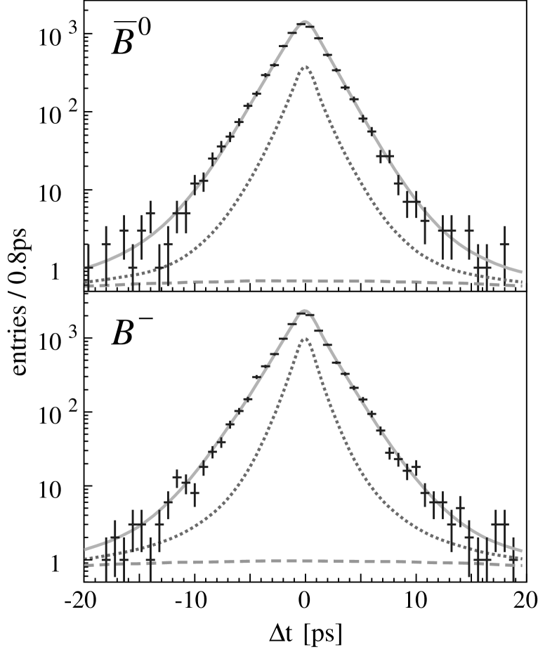
The resulting $\Delta t$ resolution for the signal is $\sim 1.56~{}{\rm ps}$ (rms) for this data sample. Figure 16 shows the distributions of $\Delta t$ for ${\overline{B}{}^{0}}$ and ${B^{-}}$ events in the signal region with the fitted curves superimposed. The systematic errors arising from the resolution functions are estimated by comparing the results obtained using a different functional form and by varying the resolution parameters within their errors. They amount to $0.010$ ps, $0.009$ ps and $\ 0.006$ for ${\tau_{{\overline{B}{}^{0}}}}$, ${\tau_{{B^{-}}}}$ and ${{\tau_{{B^{-}}}}/{\tau_{{\overline{B}{}^{0}}}}}$, respectively. MC simulation studies show no bias arising from the resolution function in the obtained results.

Table 5: The parameters determined by the lifetime fit.

	Parameters	Values
	${\tau_{{\overline{B}{}^{0}}}}$ (ps)	$1.554\pm 0.030$
	${\tau_{{B^{-}}}}$ (ps)	$1.695\pm 0.026$
	$s_{\rm ful}^{0}$	$0.809\pm 0.148$
	$s_{\rm ful}^{1}$	$0.154\pm 0.013$
	$s_{\rm asc}^{0}$	$0.753\pm 0.065$
	$s_{\rm asc}^{1}$	$0.064\pm 0.005$
	$s_{\rm main}$	$0.647^{+0.074}_{-0.083}$
	$s_{\rm tail}$	$3.00^{+2.23}_{-0.99}$
	$f_{\rm tail}$	$0.083^{+0.083}_{-0.045}$
	$\sigma_{{\rm ol}}$ (ps)	$36.2^{+5.0}_{-3.5}$
	$f_{{\rm ol}}^{\rm multiple}$	$(5.83^{+3.02}_{-2.25})\times 10^{-4}$
	$f_{{\rm ol}}^{\rm single}$	$0.0306\pm 0.0036$

Figure 16: The $\Delta t$ distributions of (a) neutral and (b) charged $B$ meson pairs, with fitted curves. The dotted lines represent the sum of the background and outlier component, and the dashed lines represent the outlier component.

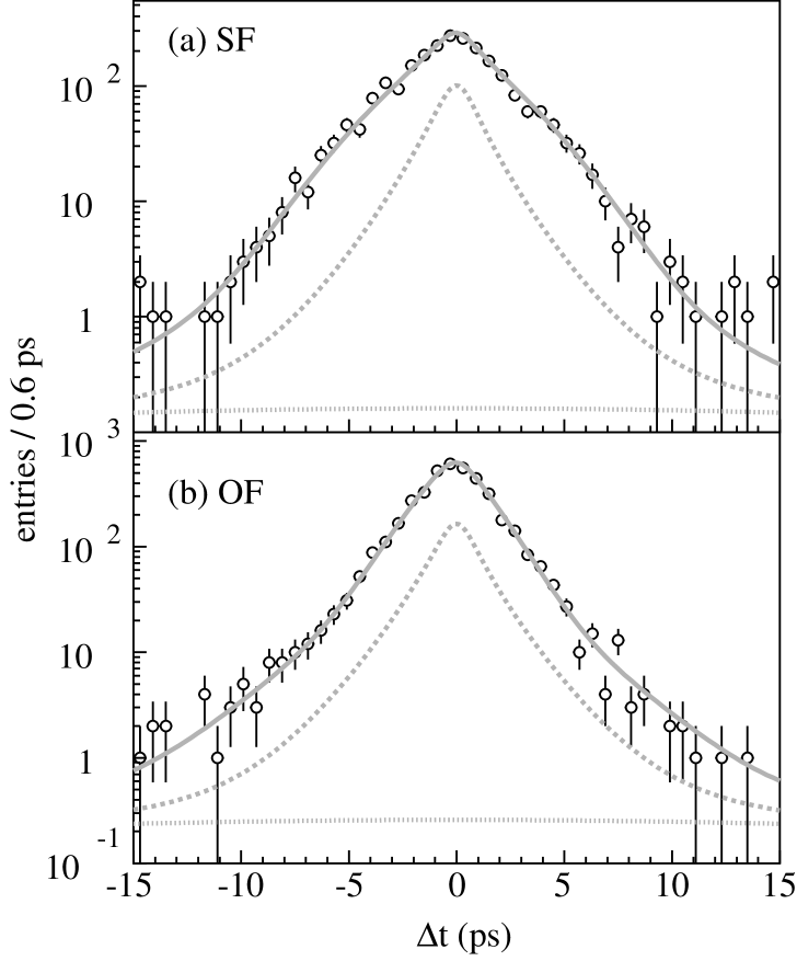
The same data sample is used to determine the $B^{0}\overline{B}{}^{0}$ oscillation frequency $\Delta m_{d}$ from the time evolution of opposite-flavor (OF; $B^{0}\overline{B}{}^{0}$) and same-flavor (SF; $B^{0}B^{0}$, $\overline{B}{}^{0}\overline{B}{}^{0}$) neutral $B$ decays [3]. The signal PDF is defined as the convolution of the true PDF,

$$\mathcal{P}^{\rm OF}(\Delta t) = \frac{1}{4\tau_{\overline{B}{}^{0}}}\exp\left(-\frac{|\Delta t|}{\tau_{\overline{B}{}^{0}}}\right)[1+(1-2w)\cos(\Delta{m_{d}}\Delta t)]\ \ {\rm and}$$

$$\mathcal{P}^{\rm SF}(\Delta t) = \frac{1}{4\tau_{\overline{B}{}^{0}}}\exp\left(-\frac{|\Delta t|}{\tau_{\overline{B}{}^{0}}}\right)[1-(1-2w)\cos(\Delta{m_{d}}\Delta t)],$$ (31)

with the resolution function $R_{{\rm sig}}(\Delta t)$. Here $w$ is the probability for an incorrect flavor assignment and determined simultaneously with $\Delta m_{d}$ by the fit. Figure 17 shows the $\Delta t$ distributions for OF and SF events with fitted curves superimposed. The fit yields

$$\Delta m_{d}=0.528\pm 0.017({\rm stat})\pm 0.011({\rm syst})\ \ {\rm ps}^{-1}.$$

The error arising from the resolution function accounts for $0.009$ ps^-1 of the total systematic error quoted above.

Figure 17: The $\Delta t$ distributions for (a) SF and (b) OF events with the fitted curves superimposed. The dashed, dotted, and solid curves show the background, outliers, and the sum of backgrounds and signal, respectively.

5.2 Time-dependent $CP$ asymmetry

The resolution function obtained above is also used for the measurement of mixing-induced $CP$ violation in the neutral $B$ meson system. The Standard Model predicts a $CP$-violating asymmetry in the time-dependent rates for $B^{0}$ and $\overline{B}{}^{0}$ decays to a common $CP$ eigenstate $f_{CP}$, where the transition is dominated by the $b\to c\bar{c}s$ process:

$$A(t)\equiv\frac{\Gamma({\overline{B}{}^{0}}\to f_{CP})-\Gamma({B^{0}}\to f_{CP})}{\Gamma({\overline{B}{}^{0}}\to f_{CP})+\Gamma({B^{0}}\to f_{CP})}=-\xi_{f}\sin 2\phi_{1}\sin(\Delta m_{d}t),$$ (32)

where $\Gamma({B^{0}},{\overline{B}{}^{0}}\to f_{CP})$ is the decay rate for ${B^{0}}$ or ${\overline{B}{}^{0}}$ to $f_{CP}$ at a proper time $t$ after production, $\xi_{f}$ is the $CP$ eigenvalue of $f_{CP}$, and $\sin 2\phi_{1}$ is the $CP$ violation parameter. A non-zero value for $\sin 2\phi_{1}$ establishes that $CP$ symmetry is violated in the neutral $B$ meson system. We use events in which one of the $B$ mesons decays to $f_{CP}$ at time $t_{CP}$, and the other decays to a self-tagging state $f_{\rm tag}$, which distinguishes ${B^{0}}$ from ${\overline{B}{}^{0}}$, at time $t_{\rm tag}$. The $CP$ violation manifests itself as an asymmetry $A(\Delta t)$, where $\Delta t$ is the proper time interval between the two decays: $\Delta t\equiv t_{CP}-t_{\rm tag}$.

The PDF expected for the signal distribution is

$$\mathcal{P}_{\rm sig}(\Delta t,q,w,\xi_{f})=\frac{1}{4{\tau_{{\overline{B}{}^{0}}}}}\exp\left(-\frac{|\Delta t|}{{\tau_{{\overline{B}{}^{0}}}}}\right)[1-q\xi_{f}(1-2w)\sin 2\phi_{1}\sin(\Delta m_{d}\Delta t)],$$ (33)

where $q$ has the discrete value $+1(-1)$ when the tag-side $B$ meson is likely to be a $B^{0}$ ($\overline{B}{}^{0}$), and $w$ is, as mentioned in the previous section, the probability for an incorrect flavor assignment (wrong-tag probability) [9]. The PDF is convolved with $R_{{\rm sig}}(\Delta t)$ to determine the likelihood value for each event as a function of $\sin 2\phi_{1}$:

$$P_{i} = (1-f_{{\rm ol}})[f_{{\rm sig}}\int\mathcal{P}_{\ sig}(\Delta t^{\prime},q,w,\xi_{f})R_{{\rm sig}}(\Delta t-\Delta t^{\prime}){\rm d}\Delta t^{\prime}$$ (34)

$$\quad+\;(1-f_{{\rm sig}})P_{\rm bkg}(\Delta t)]+f_{{\rm ol}}P_{{\rm ol}}(\Delta t).$$

The only free parameter in the final fit is $\sin 2\phi_{1}$. The quality of the vertex fit for the tag-side $B$ meson (or associated $B$ meson) can be correlated with $w$, and, therefore, the resolution function can also be correlated with $w$ primarily because of smearing due to non-primary tracks. $R_{{\rm np}}$ is designed to account for this correlation by making the parameters of vertex position shifts ($\tau_{\rm np}^{\rm p}$ and $\tau_{\rm np}^{\rm n}$) a function of vertex-fit qualities ($\sigma_{\rm acs}$ and $\xi_{\rm asc}$). MC simulation study shows that the remaining $w$ dependence is negligible.

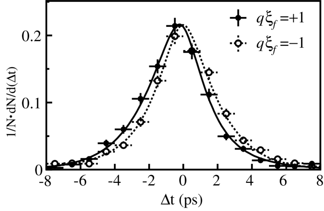
The value of $\sin 2\phi_{1}$ is measured using a $78~{}{\rm fb}^{-1}$ data sample, which contains 85 million $B\overline{B}$ pairs [4]. This data sample has been analyzed using a new track reconstruction algorithm that provides better performance in vertex reconstruction. We repeat the lifetime fit to this sample to determine the parameter values for $R_{{\rm sig}}(\Delta t)$. We find the fraction $f_{\rm tail}$ for the tail part of the detector resolution is consistent with zero, and therefore set $f_{\rm tail}=0$ for this data sample. In addition, the improvement in statistics enables us to determine some parameters that are previously determined only by MC simulations. The fractions of the prompt component in $R_{{\rm np}}$ for multiple- and single-track vertices ($f_{\delta,\overline{B}{}^{0}}^{\rm multiple}$, $f_{\delta,\overline{B}{}^{0}}^{\rm single}$ for $\overline{B}{}^{0}$ mesons, and $f_{\delta,B^{-}}^{\rm multiple}$, $f_{\delta,B^{-}}^{\rm single}$ for $B^{-}$ mesons) are determined by the lifetime fit to the data. The values so obtained are consistent with the values determined using MC simulations. Table 6 lists the parameter values for $R_{{\rm sig}}(\Delta t)$. We find the resulting $\Delta t$ resolution to be $\sim 1.43~{}{\rm ps}$ (rms), improved over the resolution of $\sim 1.56~{}{\rm ps}$ obtained for the $29~{}{\rm fb}^{-1}$ sample. Figure 18 shows the observed $\Delta t$ distributions for $q\xi_{f}=+1$ (solid points) and $q\xi_{f}=-1$ (open points) event samples. The asymmetry between the two distributions is proportional to $\sin 2\phi_{1}$ and demonstrates the violation of $CP$ symmetry. The value of $\sin 2\phi_{1}$ is measured to be

$$\sin 2\phi_{1}=0.719\pm 0.074{\rm(stat)}\pm 0.035{\rm(syst)}.$$

The quoted systematic error includes the systematic error due to the uncertainty in the resolution function ($0.014$).

Table 6: The resolution function parameters determined using a $78~{}{\rm fb}^{-1}$ data sample. This data sample has been analyzed using a new track reconstruction algorithm.

	Parameters	Values
	${\tau_{{\overline{B}{}^{0}}}}$ (ps)	$1.551\pm 0.018$
	${\tau_{{B^{-}}}}$ (ps)	$1.658\pm 0.016$
	$s_{\rm ful}^{0}$	$0.987^{+0.117}_{-0.124}$
	$s_{\rm ful}^{1}$	$0.094\pm 0.008$
	$s_{\rm asc}^{0}$	$0.778\pm 0.048$
	$s_{\rm asc}^{1}$	$0.044\pm 0.002$
	$s_{\rm main}$	$0.972\pm 0.045$
	$\sigma_{{\rm ol}}$ (ps)	$42.0^{+4.6}_{-3.5}$
	$f_{{\rm ol}}^{\text{multiple}}$	$(1.65^{+1.13}_{-0.82})\times 10^{-4}$
	$f_{{\rm ol}}^{\text{single}}$	$0.0269\pm 0.0019$
	$f_{\delta,{\overline{B}{}^{0}}}^{\text{multiple}}$	$0.555\pm 0.042$
	$f_{\delta,{B^{-}}}^{\text{multiple}}$	$0.440\pm 0.046$
	$f_{\delta,{\overline{B}{}^{0}}}^{\text{single}}$	$0.701\pm 0.040$
	$f_{\delta,{B^{-}}}^{\text{single}}$	$0.764\pm 0.044$

Figure 18: The $\Delta t$ distributions for the events with $q\xi_{f}=+1$ (solid points) and $q\xi_{f}=-1$ (open points). The results of the global fit with $\sin 2\phi_{1}=0.719$ are shown as solid and dashed curves, respectively. See text for the detail.

6 Conclusions

The resolution function, which is used in an unbinned maximum likelihood fit for the time-dependent measurements at the Belle experiment, is studied in detail. The resolution function is described as a convolution of three components; the detector resolution, the smearing due to non-primary tracks, and the kinematic approximation. The functional forms to describe these components are determined based on detailed MC simulation studies. The parameters for the detector resolution are determined using the data. The resulting resolution function has successfully described the $\Delta t$ distribution used for measurements of $B$ meson lifetimes, ${B^{0}}{\overline{B}{}^{0}}$ oscillation frequency, and the mixing-induced CP asymmetry parameter $\sin 2\phi_{1}$.

References

• [1] S. Kurokawa and E. Kikutani, Nucl. Instr. and Meth. A 499, 1 (2003).
• [2] Belle Collaboration, K. Abe et al., Phys. Rev. Lett. 88, 171801 (2002).
• [3] Belle Collaboration, T. Tomura et al., Phys. Lett. B 542, 207 (2002).
• [4] Belle Collaboration, K. Abe et al., Phys. Rev. D 66, 071102(R) (2002).
• [5] Belle Collaboration, A. Abashian et al., Nucl. Instr. and Meth. A 479, 117, (2002).
• [6] R. Abe et al., IEEE Trans. Nucl. Sci. 48, 997 (2001).
• [7] The QQ B𝐵B meson decay event generator was developed at the CLEO Collaboration. http://www.lns.cornell.edu /public/CLEO/soft/QQ.
• [8] CERN Program Library Long Writeup W5013, CERN (1993).
• [9] H. Kakuno et al., hep-ex/0403022, to appear in Nucl. Instr. and Meth.